Radiative effects in the standard model extension

Abstract

The possibility of radiative effects induced by the Lorentz and CPT non-invariant interaction term for fermions in the standard model extension is investigated. In particular, electron-positron photo-production and photon emission by electrons and positrons are studied. The rates of these processes are calculated in the Furry picture. It is demonstrated that the rates obtained in the framework of the model adopted strongly depend on the polarization states of the particles involved. As a result, ultra-relativistic particles produced should occupy states with a preferred spin orientation, i.e., photons have the sign of polarization opposite to the sign of the effective potential, while charged particle are preferably in the state with the helicity coinciding with the sign of the effective potential. This leads to evident spatial asymmetries which may have certain consequences observable at high energy accelerators, and in astrophysical and cosmological studies.

I Introduction

Physical laws have been confirmed to be Lorentz invariant with high accuracy in numerous experiments 1 . Nevertheless, for the last few years there have been made a number of assumptions that these symmetries are only approximate.

The modern quantum field theoretical viewpoint admits the possibility of Lorentz invariance breaking (and, as a consequence, possible CPT invariance breaking in the local field theory) through a spontaneous symmetry breaking mechanism. In other words, even though the underlying laws of nature have Lorentz and CPT symmetries, the vacuum solution of the theory could spontaneously violate these symmetries.

The Standard Model does not have dynamics necessary to cause spontaneous Lorentz and CPT violation. However, the violation mentioned above could occur in more fundamental theories, such as string theories, noncommutative geometry, etc., and the resulting theory can be effectively described in the framework of the standard model extension (SME) 2 .

At present, there are numerous approaches to study various effects of possible Lorentz violation. However, the SME is the most consistent of all in describing theoretical implications of the Lorentz violation hypothesis (for a recent review of SME, see, e.g., new ). It is in the framework of this theory that calculations have been performed teor , whose results became the basis for experimental verification of Lorentz invariance in the low energy range exp .

It is surprising though that the high energy consequences of this theory have not been studied as yet, whereas the possible effects in this range are expected to be more substantial, than those at low energy. Some estimates of the rates of certain electromagnetic processes have been obtained only at the phenomenological level (see, e.g., 1c and references therein). In the present publication, we attempted to partly compensate for this lack of theoretical estimates.

The SME is fairly complicated even in the electromagnetic sector, and hence we restricted ourselves to studying only those consequences of the theory that are due to axial-vector interaction of fermions with the constant background field $b^{\mu}$ with the CPT-odd interaction term in the fermion Lagrangian $\overline{\psi}b_{\mu}\gamma^{\mu}\gamma_{5}\psi$ (notations generally excepted in the framework of the SME 2 ). This kind of modification of QED in the fermion sector does not influence the gauge invariance of the action and of the equations of motion, but it does modify the dispersion relations for Dirac spinors 2 . The question about the possible dynamical origin of this constant vector $b^{\mu}$ remains an interesting task to be solved. One of the possibilities is that the pseudovector field $b^{\mu}$ might be related to some constant background torsion in the large scale Universe, $b^{\mu}\sim\varepsilon^{\mu\nu\lambda\delta}T_{\nu\lambda\delta}$ 6 . Moreover, such a CPT-odd term could be generated by chiral fermions 7 .

This model has been extensively employed in numerous publications 9 ; 10 ; 11 ; 12 ; 13 ; 14 , where the Chern–Simons term generated by the fermion loop in the $b^{\mu}$ background was studied. The results of these studies have been controversial, since they depended on the type of regularization adopted during calculations. The final conclusion can only be drawn after certain additional physical assumptions have been made. New interesting results at finite temperature have also been obtained, — for instance, the Chern–Simons term vanishes in the very high temperature limit 15 . The applications of the SME predictions to astrophysics and cosmology are also of interest 1c (see, also 14 , where, in particular, energy splitting between electrons of different helicities and decay of very high energy electrons into lower energy electrons and positrons have been considered). It should also be mentioned that this type of axial-vector interaction arises in the study of the coherent interaction of neutrino with dense matter in the framework of the Standard Model (see, e.g., 16 ).

The parameter $b^{\mu}$ as a 4-vector may be time-like or space-like. In what follows, we shall consider the first possibility. The experimental bounds for the space components of $b^{\mu}$ are rather stringent, i.e., $|{\bf b}|<10^{-18}$–$10^{-20}$eV, or even stronger, depending on the type of the experiment (for more details of the experimental situation, see exp ; new , and references therein). Interesting enough is the fact that no stringent experimental limitations for the time component $b^{0}$ (at least for an electron, and this case is just of interest for us) have yet been obtained. One may argue (see, e.g., 14 ) that, since the precision for measurements of the electron mass is about $10^{-8}$, the upper bound on the time component may be $|b_{0}|<10^{-2}$eV.

In the present work we investigate the possibility of electron-positron pair production by a photon and radiation of a photon by electrons and positrons induced by the Lorentz breaking background $b^{0}$. We assume that the photon dispersion law remains unchanged, and hence we neglect Cherenkov radiation. Our calculations are made in the framework of the Furry picture F51 , i.e., we consider the Lorentz breaking axial vector background as a kind of an external field and take it into consideration exactly, i.e., without making any expansion in powers of the parameter $b^{0}.$ This means that creation and annihilation operators are exact solutions of the Dirac equation in the external or condensate field and form the basis for the perturbation theory description of interaction with the radiation field. This technique is appropriate when external or condensate fields are strong and particle energies are high. Moreover, since the dispersion law for charged particles in the external or condensate field changes as compared with the zero field case, new channels of reactions may become open. The calculations with this basis are, however, quite complicated. Nevertheless, it is with the use of this technique that various processes feasible in the astrophysics, such as one-photon electron-positron pair production, photon splitting, beta-decay in the strong magnetic field of pulsars, and a number of others were investigated (see, e.g., klepikov ; adler ; ritus ; shabad ; L16 ; ZZ ; for the recent reviews of such calculations, see kniga ; BVZ97 ).

II The Model

Consider fermions interacting with an electromagnetic field $A^{\mu}(x)$ and with a constant condensate field $b^{\mu}$. The Lagrangian density of the model 2 is as follows:

$${\cal L}={\cal L}_{\rm{em}}+{\cal L}_{\rm{Dir}},$$ (1)

where

$${\cal L}_{\rm{em}}=-\frac{1}{4}F_{\mu\nu}F^{\mu\nu}$$ (2)

is the electromagnetic field Lagrangian and

$${\cal L}_{\rm{Dir}}=\overline{\psi}(i\gamma^{\mu}\partial_{\mu}+e\gamma^{\mu}A_{\mu}-m-b_{\mu}\gamma^{\mu}\gamma_{5})\psi$$ (3)

is the Lagrangian of the Dirac field.

In order to calculate the rate of pair photo-production and the rate of radiative transition of an electron induced by the Lorentz breaking background in the framework of the Furry picture, the “extended” Dirac equation that takes into account interaction with the axial vector term should be solved. As it follows from the SME Lagrangian (3), the Dirac equation has the form

$$\left(i{\gamma^{\mu}{\partial}_{\mu}}-\gamma^{\mu}{b_{\mu}}\gamma^{5}-m\right)\psi=0.$$ (4)

The canonical momentum operator $i{{\partial}^{\mu}}$ commutes with the operator of equation (4). It can be shown (see L05 ) that the eigenvalues of the operator $i\partial^{\mu}$ are as follows:

$$P^{\mu}=q^{\mu}\left(1+\frac{\zeta b^{2}}{\sqrt{(bq)^{2}-b^{2}m^{2}}}\right)+{b^{\mu}}\left(1-\frac{\zeta(bq)}{\sqrt{(bq)^{2}-b^{2}m^{2}}}\right),$$ (5)

where $q^{\mu}$ is a constant 4-vector, such as $q^{2}=m^{2},$ and $\zeta=\pm 1$. The dispersion law that follows from eq. (5) has the form

$$P^{2}=m^{2}+2(Pb)-2{b^{2}}-2\zeta\sqrt{\left((Pb)-{b^{2}}\right)^{2}-b^{2}m^{2}}.$$ (6)

Consider now the most interesting case of a time-like vector $b^{\mu}$ and choose it in the form $b^{\mu}=\{b,0,0,0\}.$ In this case the orthonormalized system of solutions of equation (4) can be written as follows:

$$\psi(x)=\frac{\left|\Delta_{q\zeta}\right|}{\sqrt{2q^{0}}}\,e^{-iq^{0}x^{0}}e^{i{\bf{qx}}\Delta_{q\zeta}}(\gamma^{\mu}{q_{\mu}}+m)(1-\zeta\gamma^{5}\gamma_{\nu}{S}^{\nu}_{tp})\psi^{0},$$ (7)

where $\psi^{0}$ is a constant bispinor, $\Delta_{q\zeta}=1+\zeta b/|{\bf{q}}|,$ and

$$S_{tp}^{\mu}=\frac{1}{m}\left\{|{\bf q}|,q^{0}{\bf q}/|{\bf q}|\right\}.$$ (8)

It is easily seen that the 4-vector $q^{\mu}=\{q^{0},{\bf q}\}$ plays the role of the kinetic momentum of the particle with the energy $\varepsilon=q^{0}$ given by the same dispersion relation as in the case of a free particle in the Lorentz invariant theory

$$\varepsilon=\sqrt{{\bf q}^{2}+m^{2}}.$$ (9)

It is clear that in this case the relation between the canonical momentum $\bf{P}$ and the kinetic momentum $\bf{q}$ is determined by the formula

$${\bf P}={\bf q}\Delta_{q\zeta},$$ (10)

and consequently, the dispersion law can be rewritten in the form

$$\varepsilon=\sqrt{\left(\Delta|{\bf{P}}|-\zeta b\right)^{2}+m^{2}},$$ (11)

where $\Delta={\mathrm{sign}\left(\Delta_{q\zeta}\right)}$ is the sign factor. It is therefore clear that

$${\bf v}=\frac{\partial\varepsilon}{\partial{\bf{P}}}=\frac{\bf{q}}{q^{0}}$$ (12)

is the particle group velocity.

The relation (11) differs from those used in papers 16 by the sign factor $\Delta.$ This is due to the fact that, in those papers, the canonical momentum ${\bf{P}}$ and not the kinetic momentum ${\bf q}$ was used as the particle quantum number, and $\zeta$ was the projection of the particle spin on the canonical momentum. It should be emphasized however, that the particle kinetic momentum components, related to the group 4-velocity $u^{\mu}$ by the relation $q^{\mu}=mu^{\mu},$ $q^{2}=m^{2},$ and not the canonical momentum components, are suitable to play the role of the particle quantum numbers. Moreover, we choose the helicity of the particle as the spin quantum number $\zeta$. It is well known that for a particle in an external field, the projection of its spin on the direction of its kinetic momentum is defined as its helicity ST ; BG ; T . In our problem the directions of canonical and kinetic momenta are different, and hence, the projection of particle spin on the canonical momentum does not coincide with its helicity. Thus, we believe that the particle kinetic momentum, related to its group velocity (12), and its helicity are the particle physical variables that can be considered as its observables. This justified our decision that they should be taken as the particle quantum numbers.

III Pair production

Consider the electron-positron pair photo-production process. The probability of pair production by a polarized photon is defined by the relation

$$\begin{array}[]{c}\displaystyle W=\frac{1}{2k^{0}}\!\int\!\!d^{4}x\,d^{4}y\!\int\frac{d^{4}p\,d^{4}q}{(2\pi)^{6}}\,\delta(p^{2}\!-m^{2})\delta(q^{2}\!-m^{2})\\[8.0pt] \displaystyle\times{\mathrm{Sp}}\big{\{}\gamma_{\mu}(x)\varrho_{\bar{e}}(x,y;p,\zeta_{p})\gamma_{\nu}(y)\varrho_{e}(y,x;q,\zeta_{q})\big{\}}\varrho^{\mu\nu}_{ph}(y,x;k).\end{array}$$ (13)

Here, $\varrho_{e}(y,x;q,\zeta_{q}),\varrho_{\bar{e}}(x,y;p,\zeta_{p})$ are the electron and positron density matrices respectively, $\,\varrho^{\mu\nu}_{ph}(y,x;k)$ is the density matrix of the initial photon with 4-momentum $k^{\mu}$. The density matrices of longitudinally polarized electron with the 4-momentum $q^{\mu}$ and helicity $\zeta_{q}$ and positron with 4-momentum $p^{\mu}$ and helicity $\zeta_{p}$ in the Lorentz breaking background constructed with the use of solutions (7) have the form

$$\begin{array}[]{c}\displaystyle\varrho_{\bar{e}}(x,y;p,\zeta_{p})=\frac{1}{2}\Delta_{p\zeta_{p}}^{2}(\gamma^{\mu}{p_{\mu}}-m)(1-\zeta_{p}\gamma^{5}\gamma_{\nu}{S}^{\nu}_{tp}(p))\displaystyle e^{i(x^{0}-y^{0})p^{0}-i({\bf x}-{\bf y}){\bf p}\Delta_{p\zeta_{p}}},\\[8.0pt] \displaystyle\varrho_{{e}}(y,x;q,\zeta_{q})=\frac{1}{2}\Delta_{q\zeta_{q}}^{2}(\gamma^{\mu}{q_{\mu}}+m)(1-\zeta_{q}\gamma^{5}\gamma_{\nu}{S}^{\nu}_{tp}(q))\displaystyle e^{i(x^{0}-y^{0})q^{0}-i({\bf x}-{\bf y}){\bf q}\Delta_{q\zeta_{q}}}.\end{array}$$ (14)

Upon integrating with respect to coordinates, we obtain the following expression for the transition rate under investigation:

$$\begin{array}[]{c}\displaystyle W=\frac{e^{2}}{k^{0}}\!\!\int\frac{d^{4}p\,d^{4}q}{2\pi}\,\delta(p^{2}\!-m^{2})\delta(q^{2}\!-m^{2})\delta(k^{0}-p^{0}-q^{0})\delta^{3}({\bf k}-{\bf p}\Delta_{p\zeta_{p}}-{\bf q}\Delta_{q\zeta_{q}})T(p,q).\end{array}$$ (15)

Here

$$T(p,q)=\displaystyle\frac{1}{4}{\mathrm{Sp}}\left\{\gamma^{\alpha}{e_{\alpha}}(\gamma^{\mu}{p}_{\mu}-m)(1-\zeta_{p}\gamma^{5}\gamma_{\nu}{S}^{\nu}_{tp}(p)){\gamma^{\beta}{e}^{*}_{\beta}}(\gamma^{\rho}{q_{\rho}}+m)(1-\zeta_{q}\gamma^{5}\gamma_{\lambda}{S}^{\lambda}_{tp}(q))\right\},$$ (16)

where $e^{\mu}=\left\{0,{\bf a}_{1}+ig{\bf a}_{2}\right\}/{\sqrt{2}}$, with $g=\pm 1$, are unit vectors of circular polarization.

Instead of the electron, positron and photon energies $\varepsilon_{{e}}\equiv q^{0},\,\varepsilon_{\bar{e}}\equiv p^{0},\varepsilon_{\gamma}\equiv k^{0}$ respectively, and polarizations $\zeta_{q},\,\zeta_{p},\,g,$ and the effective potential $b$, it is convenient to introduce the dimensionless quantities

$$\begin{array}[]{llll}\eta=k^{0}/2m,&\eta+y=p^{0}/m,&\eta-y=q^{0}/m,&{}\\[4.0pt] \bar{g}={g}\,{\mathrm{sign}}(b),&\bar{\zeta}_{\bar{e}}={\zeta}_{p}\,{\mathrm{sign}}(b),&\bar{\zeta}_{e}={\zeta}_{q}\,{\mathrm{sign}}(b),&d=|b|/m.\end{array}$$ (17)

Then the results of integration in (15) can be expressed in the form

$$\begin{array}[]{c}\displaystyle W_{\bar{g}\bar{\zeta}_{\bar{e}}\bar{\zeta}_{e}}=\frac{e^{2}m}{32\eta^{2}}\int\!\!\frac{dy}{\sqrt{(\eta+y)^{2}-1}\sqrt{(\eta-y)^{2}-1}}\\[12.0pt] \displaystyle\times\left[\bar{\zeta}_{\bar{e}}\sqrt{(\eta+y)^{2}-1}+\bar{\zeta}_{e}\sqrt{(\eta-y)^{2}-1}+2d+2\bar{g}\eta\right]^{2}.\end{array}$$ (18)

The integration limits in the above formula depend on the values of parameter $d.$ In the realistic limit of small $d\ll 1$, for the case $\bar{\zeta}_{\bar{e}}=1,\bar{\zeta}_{{e}}=1,$ we have x

$$\begin{array}[]{ll}y\in\varnothing&\quad\eta\in[1,\eta_{1}),\\ y\in[-y_{0},y_{0}]&\quad\eta\in[\eta_{1},\infty),\end{array}$$ (19)

and for other values of $\bar{\zeta}_{\bar{e}}$ and $\bar{\zeta}_{e}$

$$\begin{array}[]{ll}y\in\varnothing&\quad\eta\in[1,\infty),\end{array}$$ (20)

where

$$\eta_{1}=\frac{1+d^{2}}{2d},\qquad y_{0}=\frac{|\eta-d|\sqrt{\eta-\eta_{1}}}{\sqrt{\eta-d/2}}.$$ (21)

In other words, there exists a threshold $\eta_{1}$, depending on the parameter $b$, such that only for $\eta\geqslant\eta_{1}$ the process can take place. This is natural for the $e^{+}e^{-}$ pair production process in the background field. Moreover, as it is seen from (17), (19), (20), only those electrons and positrons can be produced, whose helicities are equal and whose sign coincide with the sign of the effective potential $b$.

Then, upon integrating over $y$, one obtains the transition rate

$$W_{\bar{g}\bar{\zeta}_{\bar{e}}\bar{\zeta}_{e}}=\frac{e^{2}m}{32\eta^{2}}(1+\bar{\zeta}_{\bar{e}})(1+\bar{\zeta}_{{e}})\Theta(\eta-\eta_{1})\,J.$$ (22)

Here $\Theta(\eta-\eta_{1})$ is the Heaviside step function and

$$\begin{array}[]{c}\displaystyle J=\left[2(\eta+\bar{g}d)+d^{2}/\eta\right]F(\chi,s)-\eta E(\chi,s)\\[8.0pt] +\displaystyle y_{0}\left[1+\frac{\sqrt{\left((\eta-y_{0})^{2}-1\right)}\sqrt{\left((\eta+y_{0})^{2}-1\right)}}{{y_{0}^{2}+\eta^{2}-1}}\,\right]\\[12.0pt] \displaystyle+2\left(d+\bar{g}\eta\right)\ln\frac{\sqrt{\left((\eta+y_{0})^{2}-1\right)}+\eta+y_{0}}{\sqrt{\left((\eta-y_{0})^{2}-1\right)}+\eta-y_{0}},\end{array}$$ (23)

where $F(\chi,s),E(\chi,s)$ are the elliptic integrals BE of the arguments

$$\chi=\arcsin\frac{2y_{0}\eta}{y_{0}^{2}+\eta^{2}-1},\qquad s=\sqrt{1-\eta^{-2}}\,.$$ (24)

In the limit of small $d\ll 1,$ the following expression can be obtained from (22)

$$W_{\bar{g}\bar{\zeta}_{\bar{e}}\bar{\zeta}_{e}}\approx\frac{e^{2}m}{16\eta}\,\ln\frac{1+\sqrt{1-\eta_{1}/\eta}}{1-\sqrt{1-\eta_{1}/\eta}}(1+\bar{\zeta}_{\bar{e}})(1+\bar{\zeta}_{{e}})(1+\bar{g}).$$ (25)

Near the reaction threshold $\eta=\eta_{1}\approx({2d})^{-1}$, the transition rate is described by the formula

$$W_{\bar{g}\bar{\zeta}_{\bar{e}}\bar{\zeta}_{e}}\approx\frac{e^{2}m}{8\eta}\,\sqrt{1-\eta_{1}/\eta}(1+\bar{\zeta}_{\bar{e}})(1+\bar{\zeta}_{{e}})(1+\bar{g}),$$ (26)

and high above the threshold, with $d\eta\gg 1$, by the formula

$$W_{\bar{g}\bar{\zeta}_{\bar{e}}\bar{\zeta}_{e}}\approx\frac{e^{2}m}{16\eta}\,\ln(8d\eta)\,(1+\bar{\zeta}_{\bar{e}})(1+\bar{\zeta}_{{e}})(1+\bar{g}).$$ (27)

It follows from the last formulas (26) and (27) that, in the realistic case of small $d\ll 1$, only the photons with the helicity $g$, whose sign coincides with the sign of the effective potential, i.e., $\bar{g}=1$, can effectively produce pairs. This is why the threshold singularity in the transition rate is of the square root form, which is characteristic for the processes allowed by the angular momentum selection rule. For photons with the opposite helicity sign, the pair production is suppressed. The rate of the process as a function of the inverse photon energy is depicted in FIG. 1.

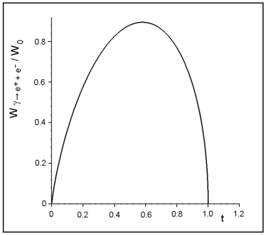
Figure 1: The rate of electron-positron pair production. $W_{0}=e^{2}m/2\eta_{1}\approx 10^{13}\left(|b|/{\mathrm{1eV}}\right){\mathrm{sec}}^{-1}$; $t=\eta_{1}/\eta\approx 2.5\cdot 10^{11}({\mathrm{1eV}})^{2}/|b|\varepsilon_{\gamma}.$

IV Photon emission

Consider now the cross-channel, i.e., photon emission by a charged particle in the Lorentz violating background. The authors of 1e proposed to call this process “helicity decay”. In fact, this is an example of the more general sort of radiation previously called “spin light” BTB95 , which is just radiation of an intrinsic magnetic moment of an electron associated with its spin. This sort of radiation has been studied for the last years in a number of papers. In the case of the “synchrotron radiation”, i.e., radiation of a relativistic charged particle in an external magnetic field, its dependence on the electron spin orientation was studied both theoretically theor and experimentally exper . As a result of these studies, it has become clear that the synchrotron radiation can be considered as consisting of two parts: one is radiation of the electron charge itself and the other is just the radiation of an intrinsic magnetic moment of an electron, and it is just what they called the “spin light”. This term was also used in L49 for the description of photon radiation by a neutrino in dense media. It should be emphasized that the mechanism of this last process (see L05 ) is similar to that of the process under investigation in the present article. As it will be seen from the formulas to follow, radiative transitions can take place both with and without the spin flip. This is why we prefer to use the term “spin light”, and not the “helicity decay” in our paper.

First of all we point out that the formulas we obtain in what follows are valid for both an electron and a positron. This is due to the fact that the sign in front of the $\gamma^{5}$ matrix in equation (4) remains invariant under the charge conjugation operation.

The rate of transition of an electron from the initial state with 4-momentum $p^{\mu}$ and helicity $\zeta_{p}$ to the final state $q^{\mu},\,\zeta_{q}$ with emission of a photon with circular polarization $g$ can be written in the form

$$W_{\bar{g}\bar{\zeta}_{i}\bar{\zeta}_{f}}=\frac{e^{2}m}{8\gamma(\gamma^{2}-1)}\int\frac{dx}{\sqrt{x^{2}-1}}\displaystyle\left[\bar{\zeta}_{i}{\sqrt{\gamma^{2}-1}}+\bar{\zeta}_{f}{\sqrt{x^{2}-1}}+2d+\bar{g}(\gamma-x)\right]^{2},$$ (28)

where instead of the initial and final electron energies $\varepsilon_{i}\equiv p^{0},\;\varepsilon_{f}\equiv q^{0}$ respectively and particle polarizations $\zeta_{p},\,\zeta_{q}$ we introduced, in addition to (17), the following dimensionless variables:

$$\gamma=p^{0}/m,\quad x=q^{0}/m,\quad\bar{\zeta}_{i}={\zeta}_{p}\,{\mathrm{sign}}(b),\quad\bar{\zeta}_{f}={\zeta}_{q}\,{\mathrm{sign}}(b).$$ (29)

The integration limits in the formula (28) are

$$\begin{array}[]{ll}x\in\varnothing&\quad\gamma\in[1,\infty),\end{array}$$ (30)

if $\bar{\zeta}_{i}=1,$ and

$$\begin{array}[]{ll}x\in\varnothing&\quad\gamma\in[1,\gamma_{0}),\\ x\in[\omega_{1},\omega_{2}]&\quad\gamma\in[\gamma_{0},\gamma_{1}),\\ x\in[1,\omega_{2}]&\quad\gamma\in[\gamma_{1},\gamma_{2}),\\ x\in\varnothing&\quad\gamma\in[\gamma_{2},\infty),\\ \end{array}$$ (31)

if $\bar{\zeta}_{i}=-1,\bar{\zeta}_{f}=-1,$ and

$$\begin{array}[]{ll}x\in\varnothing&\quad\gamma\in[1,\gamma_{1}),\\ x\in[1,\omega_{1}]&\quad\gamma\in[\gamma_{1},\gamma_{2}),\\ x\in[\omega_{2},\omega_{1}]&\quad\gamma\in[\gamma_{2},\infty),\\ \end{array}$$ (32)

if $\bar{\zeta}_{i}=-1,\bar{\zeta}_{f}=1.$

Here

$$\omega_{1}=\frac{1}{2}\left(z_{+1}+z_{+1}^{-1}\right),\qquad\omega_{2}=\frac{1}{2}\left(z_{-1}+z_{-1}^{-1}\right),$$ (33)

where

$$\begin{array}[]{l}z_{\pm 1}=\displaystyle\gamma\pm\left(\sqrt{\gamma^{2}-1}-2d\right),\end{array}$$ (34)

and

$$\begin{array}[]{ll}\gamma_{0}=\displaystyle\sqrt{1+d^{2}},&{}\\[8.0pt] \displaystyle\gamma_{1}=\frac{1}{2}\left\{\left(1+2d\right)+\left(1+2d\right)^{-1}\right\},&{}\\[12.0pt] \displaystyle\gamma_{2}=\frac{1}{2}\left\{\left(1-2d\right)+\left(1-2d\right)^{-1}\right\}.&{}\end{array}$$ (35)

As it is seen from the above formulas, radiative transitions can take place both with and without the spin flip.

The integration is carried out elementary and we obtain

$$\begin{array}[]{c}\displaystyle W_{\bar{g}\bar{\zeta}_{i}\bar{\zeta}_{f}}=\frac{e^{2}m}{16}\Big{\{}(1+\bar{\zeta}_{f})\left[Z(z_{+1},1)\Theta(\gamma-\gamma_{1})+Z(z_{-1},-1)\Theta(\gamma-\gamma_{2})\right]\\[6.0pt] \displaystyle+(1-\bar{\zeta}_{f})\left[Z(z_{+1},1)\Theta(\gamma_{1}-\gamma)+Z(z_{-1},-1)\Theta(\gamma_{2}-\gamma)\right]\Theta(\gamma-\gamma_{0})\Big{\}}(1-\bar{\zeta}_{i}).\end{array}$$ (36)

Here

$$\begin{array}[]{c}\displaystyle Z(z,\bar{\zeta}_{f})=\frac{1}{8\gamma(\gamma^{2}-1)}\Big{\{}4z_{-\bar{g}}^{2}\ln z+\Big{[}\left(z^{2}-z^{-2}\right)-\bar{g}\bar{\zeta}_{f}\left(z-z^{-1}\right)^{2}\Big{]}\\[10.0pt] -4z_{-\bar{g}}\left[\left(z-z^{-1}\right)-\bar{g}\bar{\zeta}_{f}\left(z+z^{-1}-2\right)\right]\Big{\}}.\end{array}$$ (37)

After summation over polarizations of the final particle, the transition rate becomes

$$W_{\bar{\zeta}_{f}=1}+W_{\bar{\zeta}_{f}=-1}=\frac{{e^{2}m}}{8}(1-\bar{\zeta}_{i})\Big{\{}Z(z_{+1},1)+Z(z_{-1},-1)\Big{\}}\Theta(\gamma-\gamma_{0}).$$ (38)

If $d\gamma\ll 1,$ expression (36) leads to the formula

$$W_{\bar{g}\bar{\zeta}_{i}\bar{\zeta}_{f}}\approx\frac{2e^{2}md^{3}}{3}\gamma(\gamma^{2}-1)^{1/2}(1-\bar{g}\beta)^{2}(1-\bar{\zeta}_{i})(1+\bar{\zeta}_{f}),$$ (39)

where $\beta=\sqrt{\gamma^{2}-1}/\gamma$ is the initial particle velocity.

In the relativistic limit $(\gamma\gg 1),$ the transition rate is transformed to the expression

$$W_{\bar{g}\bar{\zeta}_{i}\bar{\zeta}_{f}}\approx\frac{e^{2}m}{16\gamma}\left[\ln(1+4d\gamma)-\frac{4d\gamma(1+6d\gamma)}{(1+4d\gamma)^{2}}\right](1-\bar{\zeta}_{i})(1+\bar{\zeta}_{f})(1-\bar{g}),$$ (40)

which is valid for $d\ll 1$.

Thus, we see that at high energies $\gamma\gg 1$ charged particles radiate primarily photons with the helicity sign opposite to the sign of the effective potential $b$ (${\bar{g}}=-1$). Moreover, the radiation process is accompanied by the particle helicity flip. The rate of the process as a function of the electron inverse energy is depicted in FIG.2.

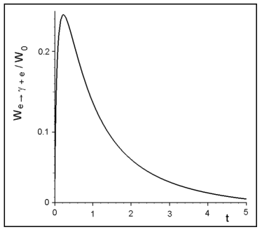
Figure 2: The rate of the radiative transition.$W_{0}=2e^{2}md\approx 2\cdot 10^{13}\left(|b|/{\mathrm{1eV}}\right){\mathrm{sec}}^{-1}$; $t=(4d\gamma)^{-1}\approx 0.6\cdot 10^{11}({\mathrm{1eV}})^{2}/|b|\varepsilon_{i}.$

Let us consider now the radiation power of spin light. If we introduce the function

$$\tilde{Z}(z,\bar{\zeta}_{f})=\gamma Z(z,\bar{\zeta}_{f})-Y(z,\bar{\zeta}_{f}),$$ (41)

where

$$\begin{array}[]{c}\displaystyle Y(z,\bar{\zeta}_{f})=\frac{1}{24\gamma(\gamma^{2}-1)}\Big{\{}-12z_{-\bar{g}}\ln z-3z_{-\bar{g}}\Big{[}\left(z^{2}-z^{-2}\right)-\bar{g}\bar{\zeta}_{f}\left(z-z^{-1}\right)^{2}\Big{]}\\[8.0pt] +\displaystyle\Big{[}(z-z^{-1})^{3}-\bar{g}\bar{\zeta}_{f}\left((z+z^{-1})^{3}-8\right)\Big{]}+6(z-z^{-1})(z_{-\bar{g}}^{2}+1)\Big{\}},\end{array}$$ (42)

then the formula for the total radiation power can be obtained from (36), (38) by substitution ${Z}(z,\bar{\zeta}_{f})\rightarrow\tilde{Z}(z,\bar{\zeta}_{f}).$ It can be verified that if $d\gamma\ll 1,$ the radiation power becomes

$$\begin{array}[]{c}\displaystyle I_{\bar{g}\bar{\zeta}_{i}\bar{\zeta}_{f}}\approx\frac{2e^{2}m^{2}d^{4}}{3}(\gamma^{2}-1)(1-\beta\bar{g})(3\gamma^{2}(1-\beta\bar{g})-1)(1-\bar{\zeta}_{i})(1+\bar{\zeta}_{f}).\end{array}$$ (43)

In the relativistic limit, the radiation power is equal to

$$\begin{array}[]{c}\displaystyle I_{\bar{g}\bar{\zeta}_{i}\bar{\zeta}_{f}}\approx\frac{e^{2}m^{2}}{16}\left[\ln(1+4d\gamma)-\frac{2d\gamma(6+15(4d\gamma)+11(4d\gamma)^{2})}{3(1+4d\gamma)^{3}}\right](1-\bar{\zeta}_{i})(1+\bar{\zeta}_{f})(1-\bar{g}).\end{array}$$ (44)

It should be first of all emphasized that as follows from our result for the radiation power (44), photons emitted by relativistic particles ($\gamma\gg 1$) are completely circulary polarized, $\bar{g}=-1$, and the helicity sign in this case is opposite to the sign of the effective potential $b$. Moreover, the total radiation power increases logarithmically. It can be seen from equations (40) and (44) that in the ultra-relativistic limit ($d\gamma\gg 1$) the average energy of emitted photons $\langle\varepsilon_{\gamma}\rangle$ is almost equal to the electron initial energy $\varepsilon_{i}$

$$\langle\varepsilon_{\gamma}\rangle\approx\varepsilon_{i}\left[1-\frac{1}{3(\ln(1+4d\gamma)-3/2)}\right].$$ (45)

It is therefore evident that the particle looses a rather significant amount of its initial energy through radiation.

V Discussion and conclusions

The results obtained demonstrate the strong dependence of the rates on the polarization properties of the particles that participate and are produced in the reactions we studied. In general, this amounts to the conclusion that, in the framework of the present model, in the ultra-relativistic limit, the particles produced in the reactions considered are preferably in the state with determined polarization, i.e., photons have the sign of polarization opposite to the sign of the effective potential, while charged particles are preferably in the state with the helicity coinciding with the sign of the effective potential. This certainly is the consequence of the particular choice of the model with Lorentz symmetry violating term in the Dirac Lagrangian we adopted. Indeed, the model assumes axial-vector interaction with the background field, and this appears to be essential to the helicity selection rules. The question arises, as to what may happen for other Lorentz structures such as vector, tensor, and chiral structures such as $(V\pm A)$ in the Lagrangian that also occur in a reasonable standard model extension. In the standard model extension 2 (we restricted ourselves to its electrodynamic sector only), interactions of particles with various condensate fields of the vector, tensor and axial-vector nature are included in the Lagrangian, and the resulting theory is renormalizable. As is known, rates of the processes in such theories should decrease with growing energy in the very high energy limit. Hence, the system in the final state should have zero orbital moment. The results of the present paper confirmed this conclusion for the particular choice of the axial-vector interaction with the background field. One may expect that with other forms of the Lorentz violating background, only those transitions would dominate that are allowed by this general selection rule. At the same time, for different types of interaction, this selection rule may lead to different correlations between the spin quantum numbers of participating particles. In the case in question, there is no specified direction in space and these correlations are quite simple. On the other hand, e.g., with the tensor type condensate determined by the parameter $H^{\mu\nu}$ in the SME Lagrangian, the fermion spin states are described by the transversal polarization rather than helicity. Therefore, for this case, any conclusions concerning spin correlation can only be made upon detailed consideration of the problem.

Due to the above mentioned polarization properties of particles produced in the reactions considered, the photon radiation process together with the pair production can not form a cascade process. Let the sign of the effective potential be positive (in the opposite case, the arguments are evident). Then as a result of the radiative transition, a photon with left polarization and an electron with arbitrary polarization are produced. However, the right-handed electron can not radiate at all, while the left-handed recoil electron, as is easily verified, will have the energy lower than the threshold value $\gamma=\sqrt{1+d^{2}}$. Moreover, the rate of the pair production by the radiated photon is practically equal to zero, as the rate of pair production by the left-handed photon is strongly, $(\sim\eta_{1}^{-2})$, suppressed as compared to the rate of pair production by the right-handed photon. Hence, the cascade process of the form

$$e\rightarrow e+\gamma\rightarrow 2e+\bar{e},$$

predicted in 14 , proves to be impossible in our model, at least in the resonance channel. Emission of radiation by charged particles produced in the process

$$\gamma\rightarrow e+\bar{e}$$

is also impossible in our model.

It should be mentioned that the results of the present work are different from corresponding estimates of papers 1c . This is due to the fact that our results were obtained with the use of exact Dirac wave functions and the corresponding dispersion law for the particle energy in the Lorentz violating background. The authors of 1c , however, without specifying any mechanism, postulated a modified dispersion law for an electron such that it became different from the vacuum one by an additional term cubic in the electron momentum. As a result, the threshold singularity of the pair creation process in 1c had the form $({1-\eta_{1}/\eta})^{3/2}$ (in the notations of our paper), and this is characteristic for the processes forbidden by the angular momentum selection rules. At the same time, the probability of photon emission by an electron in 1c increases with growing energy as $\gamma^{8}$.

As it was already mentioned in the Introduction, at present there are no serious experimental limitations for the value of parameter $b$ in the case of an electron obtained in the low energy region. Assuming, for instance, that the limitations are the same as for the neutron exp , we may come to the conclusion that the effects considered above may become significant only at energies comparable to the Planck energy $M_{{\mathrm{P}}}\sim 10^{28}{\mathrm{eV}}.$ This means that they may be important only in the study of processes that take place in the early Universe. In our calculations this corresponds to putting $d\sim m/M_{{\mathrm{P}}}.$ The actual limitations for the value of parameter $b$ can, however, be given only by experiment. The results of the present paper can provide some possible guides for obtaining the limitations on the value of $b$ in the high energy region. The threshold for the process of pair production is fairly high and hence it can be observed only in the astrophysical conditions, while the spin light can be observed already in laboratory experiments with modern accelerators.

To be particular, let us consider the following illustrative example. With consideration for the above mentioned restriction $b<10^{-2}$eV, we have for the modern machines $d\gamma\ll 1.$ Therefore, with the use of equations (39) and (43), we obtain, up to coefficient of order unity, for the transition probability and spin light power respectively

$$W_{\mathrm{SL}}\sim\frac{\alpha}{\hbar}\,mc^{2}d\,(4d\gamma)^{2},\quad I_{\mathrm{SL}}\sim\frac{\alpha}{\hbar}\,{\varepsilon_{i}}^{2}d^{2}\,(4d\gamma)^{2},$$ (46)

where $\alpha$ is the fine structure constant, and the Gaussian units were used.

Moreover, the average energy of emitted photons is defined by the formula

$$\langle\varepsilon_{\gamma}\rangle_{\mathrm{SL}}\sim\varepsilon_{i}d\gamma.$$ (47)

Now, for the same quantities in the case of synchrotron radiation, we have the following

$$W_{\mathrm{SR}}\sim\frac{\alpha}{\hbar}\,mc^{2}(H/H_{0}),\quad I_{\mathrm{SR}}\sim\frac{\alpha}{\hbar}\,{\varepsilon_{i}}^{2}(H/H_{0})^{2},$$ (48)

where $H$ is the magnetic field strength, and $H_{0}=m^{2}c^{3}/e\hbar\approx 4.41\cdot 10^{13}$G is the so called “critical”, or “Schwinger” field (see, e.g., ST ). The average energy of the synchrotron radiation photon is estimated as

$$\langle\varepsilon_{\gamma}\rangle_{\mathrm{SR}}\sim\varepsilon_{i}(H/H_{0})\gamma.$$ (49)

It is clear that in our problem, the parameter $b$ plays the same role as the parameter $H/H_{0}$ in the synchrotron radiation case. The presence of an extra small parameter $(4d\gamma)^{2}$ is due to the different mechanism of radiation in our case: a photon is emitted not by the electron charge but by its magnetic moment. Therefore, we conclude that, in experiments with relativistic electrons from modern accelerators, one may find certain limitations on the value of the parameter $b$ by searching for possible hard radiation from electrons in the straight parts of their trajectories, where no synchrotron radiation should be expected.

References

- (1) K. Hagiwara et al., Phys. Rev. D 66, 010001 (2002).
- (2) S. M. Carroll, G. B. Field, and R. Jackiw, Phys. Rev. D 41, 1231 (1990); D. Colladay and V. A. Kostelecký, Phys. Rev. D 55, 6760 (1997), hep-ph/9703464; Phys. Rev. D 58, 116002 (1998), hep-ph/9809521; S. Coleman and S. L. Glashow, Phys. Rev. D 59, 116008 (1999), hep-ph/9812418.
- (3) R. Bluhm, hep-ph/0506054.
- (4) V. A. Kostelecký and Ch. Lane, J.Math.Phys. 40 6245 (1999), hep-ph/9909542; Phys.Rev. D 60, 116010 (1999), hep-ph/9908504; R. Bluhm et. al, Phys.Rev. D 68, 125008 (2003), hep-ph/0306190.
- (5) D. F. Phillips et al., Phys. Rev. D 63, 111101 (2001); M. A. Humphrey et al., Phys. Rev. A 68, 063807 (2003), physics/0103068; M. A. Humphrey, D. F. Phillips, and R. L. Walsworth, Phys. Rev. A 62, 063405 (2000); D. Bear et al., Phys. Rev. Lett. 85, 5038 (2000); L.-S. Hou, W.-T. Ni, and Y.-C. M. Li, Phys. Rev. Lett. 90, 201101 (2003); R. Bluhm and V. A. Kostelecký, Phys. Rev. Lett. 84, 1381 (2000); F. Canè et al., Phys. Rev. Lett. 93, 230801 (2004), physics/0309070; P. Wolf et al., hep-ph/0509329.
- (6) T. Jacobson, S. Liberati, and D. Mattingly, Ann. Phys. (N.Y.) 321, 150 (2006), astro-ph/0505267; D. Mattingly, Living Rev. Relativity 8, 5 (2005), gr-qc/0502097.
- (7) I. L. Shapiro, Phys. Rept. 357, 113 (2002), hep-th/0103093.
- (8) G. E. Volovik, Pis’ma Zh. Eksp. Teor. Phys. 70, 3 (1999) [JETP Lett. 70, 1 (1999)], hep-th/9905008; G. E. Volovik and A. Vilenkin, Phys. Rev. D 62, 025014 (2000), hep-ph/9905460.
- (9) A. A. Andrianov, P. Giacconi, and R. Soldati, Grav. Cosmol. Suppl. 8N1, astro-ph/0111350; J. High Energy Phys. 02 (2002) 030.
- (10) R. Jackiw and V. A. Kostelecký, Phys. Rev. Lett. 82, 3572 (1999), hep-ph/9901358.
- (11) M. Pérez-Victoria, Phys. Rev. Lett. 83, 2518 (1999), hep-th/9905061; JHEP 04, 032 (2001).
- (12) M. Chaichian, W. F. Chen and R. Gonzalez Felipe, Phys. Lett. B 503, 215 (2001), hep-th/0010129.
- (13) J. M. Chung and P. Oh, Phys. Rev. D 60, 067702 (1999), hep-th/9812132; J. M. Chung, Phys. Rev. D 60, 127901 (1999), hep-th/9904037; J. M. Chung and B. K. Chung, Phys. Rev. D 63, 105015 (2001), hep-th/0101097.
- (14) W. F. Chen, Phys.Rev. D 60, 085007 (1999), hep-th/9903258.
- (15) D. Ebert, V. Ch. Zhukovsky, and A. S. Razumovsky, Phys. Rev. D, 70, 025003, (2004), hep-th/0401241.
- (16) P. B. Pal and T. N. Pham, Phys. Rev. D 40, 259 (1989); J. F. Nieves, Phys. Rev. D 40, 866 (1989); D. Nötzold and G. Raffelt, Nucl. Phys. B 307, 924 (1988); J. Pantaleone, Phys. Lett. B 268, 227 (1991).
- (17) W. H. Furry, Phys. Rev. 81, 115 (1951).
- (18) N. P. Klepikov, Zh. Eksp. Teor. Fiz., 26, 19 (1954). The results of this pioneer work see, e.g., in A. A. Sokolov and I. M. Ternov, Radiation from Relativistic electrons (American Institute of Physics Translations Series, New York, 1986).
- (19) S. L. Adler, Ann. Phys. (N.Y.), 67, 599 (1971).
- (20) A. I. Nikishov and V. I. Ritus, Zh. Eksp. Teor. Fiz. 46, 776 (1964)[Sov. Phys. JETP 19, 529 (1964)]; V. I. Ritus, Tr. Fiz. Inst. Akad. Nauk SSSR 111, 5 (1979) [J. Sov. Laser Research 6, 497 (1985)]; A. I. Nikishov, Tr. Fiz. Inst. Akad. Nauk SSSR 111, 152 (1979) [J. Sov. Laser Research 6, 619 (1985)].
- (21) I. A. Batalin and A. E. Shabad, Zh. Eksp. Teor. Fiz. 60, 894 (1971) [Sov. Phys. JETP 33, 483 (1971)]; A. E. Shabad, Ann. Phys. (N.Y.) 90, 166 (1975); Tr. Fiz. Inst. Akad. Nauk SSSR 192, 5 (1988) [A. E. Shabad, Polarization of the Vacuum and a Quantum Relativistic gas in an External Field (Nova Science Publ., New York, 1991)]; A. E. Shabad and V. V. Usov, Astrophys. Space Sci. 102, 327 (1984).
- (22) I. M. Ternov, V. N. Rodionov, A. E. Lobanov, and O. F. Dorofeev, Pis’ma Zh. Eksp. Teor. Fiz. 37, 288 (1983) [Sov. Phys. JETP Lett. 37, 342 (1983)]; O. F. Dorofeev, V. N. Rodionov, and I. M. Ternov, Pis’ma Zh. Eksp. Teor. Fiz. 40, 159 (1984) [Sov. Phys. JETP Lett. 40, 917 (1984)]; I. M. Ternov, V. N. Rodionov, O. F. Dorofeev, and A. E. Lobanov, Izv. Vissh. Uchebn. Zav., Fizika 29, No. 3, 82 (1986) [Sov. Phys. J. 29, 224 (1986)].
- (23) I. M. Ternov, V. R. Khalilov, and V. N. Rodionov, Interaction of Charged Particles with a Strong Electromagnetic Field (Moscow State University Press, Moscow, 1982) [in Russian].
- (24) V. Ch. Zhukovskii, O. F. Dorofeev, and A. V. Borisov, in Synchrotron Radiation Theory and its Development, edited by V. A. Bordovitsyn, Series on Synchrotron Radiation Technique and Applications – Vol. 5 (World Scientific, Singapore, 1998), pp. 350-400.
- (25) A. V. Borisov, A. S. Vshivtsev, V. Ch. Zhukovsky, and P. A. Eminov, Usp. Fiz. Nauk 167, 241 (1997) [Phys. Usp. 40, 229 (1997)].
- (26) A. E. Lobanov, Phys. Lett. B 619, 136 (2005), hep-ph/0506007.
- (27) A. A. Sokolov and I. M. Ternov, Synchrotron radiation, (Akademie-Verlag, Berlin, 1968; Pergamon Press, N.Y., 1968).
- (28) V. G. Bagrov and D. M. Gitman, Exact Solutions of Relativistic Wave Equations, (Kluwer, Dordrecht, 1990).
- (29) I. M. Ternov, Introduction to Physics of Spin of Relativistic Particles [in Russian], (Moscow State Univ. Press, Moscow, 1997).
- (30) Here, for convenience, we use the mathematical notations: for the empty set, [a,b) for the open interval, and [a,b] for the closed interval.
- (31) H. Bateman and A. Erdelyi, Higher transcendental functions, v. 3, (McGraw-Hill Book Company, Inc., New York–Toronto–London, 1955).
- (32) T. Jacobson, S. Liberati, D. Mattingly, and F. W. Stecker, Phys. Rev. Lett. 93, 021101 (2004), astro-ph/0309681.
- (33) V. A. Bordovitsyn, I. M. Ternov, and V. G. Bagrov, Usp. Fiz. Nauk 165, 1084 (1995) [Phys. Usp. 38, 1037 (1995)].
- (34) See, e.g., I. M. Ternov, V. G. Bagrov, and R. A. Rzaev, Zh. Eksp. Teor. Fiz. 46, 374 (1964) [Sov. Phys. JETP 19, 255 (1964)]; and for radiation of an electron with vacuum magnetic moment I. M. Ternov, V. G. Bagrov, and V. Ch. Zhukovsky, Vestnik Mosk. Univ., Fiz. Astron. 7, No. 1, 30 (1966) [Moscow University Physics Bulletin 21, No. 1, 21 (1966)].
- (35) S. A. Belomestnykh, A. E. Bondar, M. N. Yegorychev, V. N. Zhilich, G. A. Kornyukhin, S. A. Nikitin, et al., Nucl. Instr. & Methods in Physics Research A, 227, 173 (1984).
- (36) A. Lobanov and A. Studenikin, Phys. Lett. B 564, 27 (2003), hep-ph/0212393.