Abstract

The hadronic decays $\eta,\eta^{\prime}\to 3\pi$ and $\eta^{\prime}\to\eta\pi\pi$ are investigated within the framework of U(3) chiral effective field theory in combination with a relativistic coupled-channels approach. Final state interactions are included by deriving $s$- and $p$-wave interaction kernels for meson-meson scattering from the chiral effective Lagrangian and iterating them in a Bethe-Salpeter equation. Very good overall agreement with currently available data on decay widths and spectral shapes is achieved.

PACS:	12.39.Fe, 13.25.Jx
Keywords:	Chiral Lagrangians, coupled channels, $\eta$ and $\eta^{\prime}$.

1 Introduction

The hadronic decays of $\eta$ and $\eta^{\prime}$ offer a possibility to study symmetries and symmetry breaking patterns in strong interactions. The isospin-violating decays $\eta,\eta^{\prime}\to 3\pi$, e.g., can only occur due to an isospin-breaking quark mass difference $m_{u}-m_{d}$ or electromagnetic effects. While for most processes isospin-violation of the strong interactions is masked by electromagnetic effects, these corrections are expected to be small for the three pion decays of $\eta$ and $\eta^{\prime}$ (Sutherland’s theorem) [1] which has been confirmed in an effective Lagrangian framework [2]. Neglecting electromagnetic corrections the decay amplitude is directly proportional to $m_{u}-m_{d}$.

Moreover, the $\eta$-$\eta^{\prime}$ system offers a testing ground for chiral SU(3) symmetry in QCD and the role of both spontaneous and explicit chiral symmetry breaking, the latter one induced by the light quark masses. In the absence of $\eta$-$\eta^{\prime}$ mixing, $\eta$ would be the pure member $\eta_{8}$ of the octet of Goldstone bosons which arise due to spontaneous breakdown of chiral symmetry.

Reactions involving the $\eta^{\prime}$ might also provide insight into gluonic effects through the axial U(1) anomaly of QCD. The divergence of the singlet axial-vector current acquires an additional term with the gluonic field strength tensor that remains in the chiral limit of vanishing light quark masses. This term prevents the pseudoscalar singlet $\eta_{0}$ from being a Goldstone boson which is phenomenologically manifested in its relatively large mass, $m_{\eta^{\prime}}=958$ MeV.

An appropriate theoretical framework to investigate low-energy hadronic physics is provided by chiral perturbation theory (ChPT) [3], the effective field theory of QCD. In ChPT Green’s functions are expanded perturbatively in powers of Goldstone boson masses and small three-momenta. However, final state interactions in $\eta\to 3\pi$ have been shown to be substantial both in a complete one-loop calculation in SU(3) ChPT [4] and using extended Khuri-Treiman equations [5].

In $\eta^{\prime}$ decays final state interactions are expected to be even more important due to larger phase space and the presence of nearby resonances. It is claimed, e.g., that the exchange of the scalar resonance $a_{0}(980)$ dominates the decays $\eta^{\prime}\to\eta\pi\pi$ [6] which has been confirmed both in a full one-loop calculation utilizing infrared regularization [7] and in a chiral unitary approach [8]. In the latter work, resonances are generated dynamically by iterating the chiral effective potentials to infinite order in a BSE, whereas in [7] the effects of the $a_{0}(980)$ are hidden in a combination of coupling constants of the effective Lagrangian.

In the present investigation we extend the approach of [8] by including $p$-wave interactions. This will also allow us to obtain more realistic predictions for the decay $\eta^{\prime}\to\pi^{+}\pi^{-}\pi^{0}$, where $p$-waves can—in principle—yield sizable contributions to the decay width and Dalitz slope parameters. Furthermore, we study the implications of two very recent experiments by the KLOE [9] and the VES [10] Collaborations which have determined the Dalitz plot distributions of $\eta\to 3\pi$ and $\eta^{\prime}\to\eta\pi^{+}\pi^{-}$, respectively, with high statistics. Since these new data have not been published yet, we first present the results which we obtain by relying purely on the numbers quoted by the Particle Data Group (PDG) [11]. As a second step, we include both new experiments separately in the fit and discuss the resulting changes.

The improved analysis of $\eta,\eta^{\prime}$ hadronic decays presented here is also timely in view of the planned WASA facility at COSY [12] and MAMI-C [13] which will provide even higher statistics for these decays. More precise data will help to constrain the parameters of the Lagrangian and pose tighter constraints on the framework employed here. We will illustrate that meson-meson scattering phase shifts along with available data on $\eta,\eta^{\prime}$ hadronic decays provide a set of tight constraints which must be met by theoretical approaches.

This work is organized as follows. In the next section details of the effective Lagrangian in the U(3) framework are given. Section 3 illustrates our way of incorporating final state interactions and includes a discussion of constraints set by unitarity. In Sec. 4 we present our results based on data from [11] and the changes which arise if the new, but preliminary experimental results by KLOE [9] and VES [10] are included. A critical examination of the $\eta\to 3\pi$ data of KLOE based on purely phenomenological arguments is presented in Sec. 5. We summarize our findings in Sec. 6.

2 Effective Lagrangian

In this section we present the effective Lagrangian within the framework of U(3) chiral perturbation theory and summarize the resulting $\tilde{\pi}^{0}$-$\eta_{8}$-$\eta_{0}$ mixing [8]. Up to second order in the derivative expansion the Lagrangian for the nonet of pseudoscalar mesons ($\pi^{+/-},\tilde{\pi}^{0},K^{+/-},K^{0},\bar{K}^{0},\eta_{8},\eta_{0}$) reads (note that we do not make use of large-$N_{c}$ counting rules) [14, 15, 16]

$$\mathcal{L}^{(0+2)}=-V_{0}+V_{1}\langle\partial_{\mu}U^{\dagger}\partial^{\mu}U\rangle+V_{2}\langle U^{\dagger}\chi+\chi^{\dagger}U\rangle+iV_{3}\langle U^{\dagger}\chi-\chi^{\dagger}U\rangle+V_{4}\langle U^{\dagger}\partial^{\mu}U\rangle\langle U^{\dagger}\partial_{\mu}U\rangle,$$ (1)

where $U$ is a unitary $3\times 3$ matrix which collects the pseudoscalar fields. Its dependence on $\tilde{\pi}^{0}$, $\eta_{8}$ and $\eta_{0}$ is given by

$$U=\exp{\left(\mathop{\mathrm{diag}}\nolimits(1,-1,0)\frac{i\tilde{\pi}^{0}}{f}+\mathop{\mathrm{diag}}\nolimits(1,1,-2)\frac{i\eta_{8}}{\sqrt{3}f}+\frac{i\sqrt{2}\eta_{0}}{\sqrt{3}f}+\cdots\right)}\ .$$ (2)

The expression $\langle\dots\rangle$ denotes the trace in flavor space, $f$ is the pseudoscalar decay constant in the chiral limit and the quark mass matrix $\mathcal{M}=\mathop{\mathrm{diag}}\nolimits(m_{u},m_{d},m_{s})$ enters in the combination $\chi=2B\mathcal{M}$ with $B=-\left\langle 0\right|\bar{q}q\left|0\right\rangle/f^{2}$ being the order parameter of spontaneous chiral symmetry breaking. The coefficients $V_{i}$ are functions of the singlet field $\eta_{0}$ and can be expanded in terms of this variable

$$V_{i}\Big{[}\frac{\eta_{0}}{f}\Big{]} = v_{i}^{(0)}+v_{i}^{(2)}\frac{\eta_{0}^{2}}{f^{2}}+v_{i}^{(4)}\frac{\eta_{0}^{4}}{f^{4}}+\ldots\qquad\mbox{for}\quad i=0,1,2,4$$

$$V_{3}\Big{[}\frac{\eta_{0}}{f}\Big{]} = v_{3}^{(1)}\frac{\eta_{0}}{f}+v_{3}^{(3)}\frac{\eta_{0}^{3}}{f^{3}}+\ldots\quad$$ (3)

with expansion coefficients $v_{i}^{(j)}$ not fixed by chiral symmetry. Parity conservation implies that the $V_{i}$ are all even functions of $\eta_{0}$ except $V_{3}$, which is odd, and $V_{1}(0)=V_{2}(0)=V_{1}(0)-3V_{4}(0)=\frac{1}{4}f^{2}$ gives the correct normalization for the quadratic terms of the mesons. Thus, at a given order of the derivative expansion one obtains an infinite string of increasing powers of $\eta_{0}$ preceding each term in the Lagrangian.

In order to describe the isospin-violating decays $\eta,\eta^{\prime}\to 3\pi$, we need to work with different up- and down-quark masses and their difference $m_{u}-m_{d}$ will be parametrized by means of the renormalization scale invariant quantity

$$m_{\epsilon}^{2}=B(m_{d}-m_{u})$$ (4)

which can be expressed in terms of physical meson masses following Dashen’s theorem [17]

$$m_{\epsilon}^{2}=m_{K^{0}}^{2}-m_{K^{\pm}}^{2}+m_{\pi^{\pm}}^{2}-m_{\pi^{0}}^{2}$$ (5)

up to corrections of $\mathcal{O}(e^{2}p^{2},(m_{d}-m_{u})p^{2})$.

While in the isospin limit of equal up- and down-quark masses $\tilde{\pi}^{0}$ does not undergo mixing with the $\eta_{8}$-$\eta_{0}$ system, a non-vanishing quark mass difference $m_{u}-m_{d}$ induces $\tilde{\pi}^{0}$-$\eta_{8}$-$\eta_{0}$ mixing. The mixing of $\tilde{\pi}^{0}$, $\eta_{8}$ and $\eta_{0}$ is determined by diagonalizing both the kinetic and mass terms in the Lagrangian. Since we count the mass of the $\eta^{\prime}$ as a quantity of zeroth chiral order, the $\mathcal{O}(p^{4})$ Lagrangian

$$\mathcal{L}^{(4)}=\sum_{i}\beta_{i}(\eta_{0})\mathcal{O}_{i}$$ (6)

contributes to $\eta_{8}$-$\eta_{0}$ mixing already at leading chiral order [18]. The operators $\mathcal{O}_{i}$ can be found in [19, 18], but for completeness we will display in Appendix A those relevant for the present calculation. The functions $\beta_{i}$ can be expanded in $\eta_{0}$ in the same manner as the $V_{i}$ in Eq. (1) with expansion coefficients $\beta_{i}^{(j)}$. At leading order in isospin-breaking and at second chiral order the mass eigenstates $\pi^{0}$, $\eta$, $\eta^{\prime}$ are related to the original fields $\tilde{\pi}^{0}$, $\eta_{8}$, $\eta_{0}$ by [8]

$$\tilde{\pi}^{0} = (1+R_{\tilde{\pi}^{0}\pi^{0}})\pi^{0}+R_{\tilde{\pi}^{0}\eta}\eta+R_{\tilde{\pi}^{0}\eta^{\prime}}\eta^{\prime}$$

$$\eta_{8} = R_{8\pi^{0}}\pi^{0}+(1+R_{8\eta})\eta+R_{8\eta^{\prime}}\eta^{\prime}$$

$$\eta_{0} = R_{0\pi^{0}}\pi^{0}+R_{0\eta}\eta+(1+R_{0\eta^{\prime}})\eta^{\prime}$$ (7)

with the mixing parameters given by

$$\begin{array}[]{rlcrl}R_{8\pi^{0}}^{(0)}&=\displaystyle\frac{{m_{\epsilon}^{2}}}{\sqrt{3}({m_{\eta}^{2}}-{m_{\pi}^{2}})},&&R_{\tilde{\pi}^{0}\eta}^{(0)}&=-R_{8\pi^{0}}^{(0)},\\[15.0pt] R_{8\pi^{0}}^{(2)}&=R_{8\pi^{0}}^{(0)}\Bigl{(}R_{\tilde{\pi}^{0}\pi^{0}}^{(2)}+{\textstyle\frac{2}{3}}\Delta_{\scriptscriptstyle\mathrm{GMO}}\Bigr{)},&&R_{\tilde{\pi}^{0}\eta}^{(2)}&=-R_{8\pi^{0}}^{(0)}\Bigl{(}R_{8\eta}^{(2)}+{\textstyle\frac{2}{3}}\Delta_{\scriptscriptstyle\mathrm{GMO}}\Bigr{)},\\[10.0pt] R_{0\eta}^{(2)}&=\displaystyle\frac{4\tilde{v}_{2}^{(1)}({m_{\eta}^{2}}-{m_{\pi}^{2}})}{\sqrt{2}f^{2}{m_{0}^{2}}},&&R_{8\eta^{\prime}}^{(2)}&=\displaystyle-R_{0\eta}^{(2)}+\frac{8\beta_{5,18}^{(0)}({m_{\eta}^{2}}-{m_{\pi}^{2}})}{\sqrt{2}f^{2}},\\[15.0pt] R_{0\pi^{0}}^{(2)}&=3R_{8\pi^{0}}^{(0)}R_{0\eta}^{(2)},&&R_{\tilde{\pi}^{0}\eta^{\prime}}^{(2)}&=2R_{8\pi^{0}}^{(0)}R_{8\eta^{\prime}}^{(2)},\\[5.0pt] R_{\tilde{\pi}^{0}\pi^{0}}^{(2)}&=\displaystyle-\frac{4\beta_{5}^{(0)}{m_{\pi}^{2}}+6\beta_{4}^{(0)}({m_{\eta}^{2}}+{m_{\pi}^{2}})}{f^{2}},&&R_{0\eta^{\prime}}^{(2)}&=\displaystyle-\frac{2\beta_{4,5,17,18}^{(0)}({m_{\eta}^{2}}+{m_{\pi}^{2}})}{f^{2}},\\[12.0pt] R_{8\eta}^{(2)}&=\displaystyle-\frac{4\beta_{5}^{(0)}{m_{\eta}^{2}}+6\beta_{4}^{(0)}({m_{\eta}^{2}}+{m_{\pi}^{2}})}{f^{2}},\end{array}$$ (8)

where the superscript on $R$ denotes the chiral order and we have employed the abbreviations $\tilde{v}_{2}^{(1)}=\frac{1}{4}f^{2}-\frac{1}{2}\sqrt{6}v_{3}^{(1)}$, $\beta_{5,18}^{(0)}=\beta_{5}^{(0)}+3\beta_{18}^{(0)}/2$ and $\beta_{4,5,17,18}^{(0)}=3\beta_{4}^{(0)}+\beta_{5}^{(0)}-9\beta_{17}^{(0)}+3\beta_{18}^{(0)}$. Note that for $\beta_{5,18}^{(0)}\neq 0$ the mixing parameters given in Eq. (8), which have been derived by diagonalizing the Lagrangian, depart from the usually employed orthogonal mixing scheme for $\eta$-$\eta^{\prime}$ mixing, where $R_{8\eta^{\prime}}=-R_{0\eta}$. Isospin-breaking is known to be small, therefore terms of order $(m_{u}-m_{d})^{2}$ have been neglected. The quantity $m^{2}_{0}=2v_{0}^{(2)}/f^{2}$ is the mass of the $\eta^{\prime}$ meson in the chiral limit, $m_{\pi}^{2}=2B\hat{m}$ and $m_{\eta}^{2}=4B(m_{s}+2\hat{m})/3$ with $\hat{m}=(m_{u}+m_{d})/2$ denote the pseudoscalar meson masses at leading order, while the deviation from the Gell-Mann–Okubo mass relation for the pseudoscalar mesons is given by

$$\Delta_{\scriptscriptstyle\mathrm{GMO}}=\frac{4{m_{K}^{2}}-{m_{\pi}^{2}}-3{m_{\eta}^{2}}}{{m_{\eta}^{2}}-{m_{\pi}^{2}}}=\frac{6({m_{\eta}^{2}}-{m_{\pi}^{2}})}{f^{2}}\bigg{[}\beta_{5}^{(0)}-6\beta_{8}^{(0)}-12\beta_{7}^{(0)}+\frac{4(\tilde{v}_{2}^{(1)})^{2}}{f^{2}{m_{0}^{2}}}\bigg{]}\ ,$$ (9)

where $m_{K}^{2}=B(\hat{m}+m_{s})$.

3 Final state interactions

One-loop corrections have been shown to be important in the decay $\eta\to 3\pi$ [4], but even when they are taken into account the resulting decay width remains below the measured value [11]. In $\eta^{\prime}\to 3\pi$ one expects even larger contributions from final state interactions [8], whereas for $\eta^{\prime}\to\eta\pi\pi$ reasonable agreement with experiment can also be achieved in a perturbative approach employing infrared regularization [7]. In the present combined analysis of these three dominant hadronic decay modes of $\eta$ and $\eta^{\prime}$ we include final state interactions in a non-perturbative fashion as introduced in [8], but extending the work of [8] by taking $p$-waves into account and by improving the fit procedure for the unknown couplings in the chiral Lagrangian via Monte Carlo techniques.

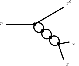
Figure 1: Shown is a possible contribution to final state interactions in the decay $\eta\to\pi^{+}\pi^{-}\pi^{0}$.

The underlying idea of our approach is that the initial particle, i.e. the $\eta$ or $\eta^{\prime}$, decays into three mesons and that two out of these rescatter (elastically or inelastically) an arbitrary number of times, see Fig. 1 for illustration. All occurring vertices are derived from the effective Lagrangian and are thus constrained by chiral symmetry. Interactions of the third meson with the pair of rescattering mesons are neglected which turns out to be a good approximation, particularly for the decays $\eta\to 3\pi$ and $\eta^{\prime}\to\eta\pi\pi$. In the decays under consideration the two-particle states either carry one elementary charge or no net charge. Charge conservation prevents transitions between these two sets, while the different channels of one set are generally coupled. There are nine uncharged combinations of mesons

$$\pi^{0}\pi^{0},\ \pi^{+}\pi^{-},\ \eta\pi^{0},\ \eta\eta,\ K^{0}\bar{K}^{0},\ K^{+}K^{-},\ \eta^{\prime}\pi^{0},\ \eta^{\prime}\eta,\ \eta^{\prime}\eta^{\prime}\,,$$ (10)

and a set of four charged channels

$$\pi^{0}\pi^{+},\ \eta\pi^{+},\ K^{+}\bar{K}^{0},\ \eta^{\prime}\pi^{+}\,.$$ (11)

For the $p$-waves there arise some simplifications in the uncharged channels. Due to Bose symmetry contributions from identical particles vanish and the remaining two-particle states can be classified according to their behavior under charge conjugation. While for $J=1$ $\pi^{+}\pi^{-}$ and $K\bar{K}$ must be $C$-odd combinations, the other pairs are $C$-even, so that transitions between the two classes of states are forbidden.

For each partial-wave $l$ unitarity imposes a restriction on the (inverse) $T$-matrix of meson-meson scattering above threshold

$$\mbox{Im}T^{-1}_{l}=-\frac{|\mbox{\boldmath$q$}_{cm}|}{8\pi E_{cm}}$$ (12)

with $E_{cm}$ and $\mbox{\boldmath$q$}_{cm}$ being the energy and the three-momentum of the particles in the center-of-mass (c. m.) frame of the channel under consideration, respectively. Hence, the imaginary part of $T^{-1}_{l}$ is equal to the imaginary piece of the fundamental scalar loop integral $\tilde{G}_{m\bar{m}}$ above threshold

$$\tilde{G}_{m\bar{m}}(p^{2})=\int\frac{\,d^{d}k}{(2\pi)^{d}}\,\frac{i}{(k^{2}-m^{2}+i\epsilon)((k-p)^{2}-\bar{m}^{2}+i\epsilon)}\ ,$$ (13)

with $m$, $\bar{m}$ denoting the masses of the two particles. In dimensional regularization the finite part $G_{m\bar{m}}$ of $\tilde{G}_{m\bar{m}}$ is given by

$$G_{m\bar{m}}(p^{2})= \mathrel{}a_{m\bar{m}}(\mu)+\frac{1}{16\pi^{2}}\bigg{[}-1+\ln\frac{m\bar{m}}{\mu^{2}}+\frac{m^{2}-\bar{m}^{2}}{p^{2}}\ln\frac{m}{\bar{m}}$$

$$\qquad\qquad\qquad\qquad\quad\mathord{}-\frac{2\sqrt{\lambda_{m\bar{m}}(p^{2})}}{p^{2}}\mathop{\mathrm{artanh}}\nolimits\frac{\sqrt{\lambda_{m\bar{m}}(p^{2})}}{(m+\bar{m})^{2}-p^{2}}\bigg{]}\ ,$$

$$\lambda_{m\bar{m}}(p^{2})= \mathrel{}\big{(}(m-\bar{m})^{2}-p^{2}\big{)}\big{(}(m+\bar{m})^{2}-p^{2}\big{)}\ ,$$ (14)

where $a_{m\bar{m}}$ is a subtraction constant which varies with the scale $\mu$ introduced in dimensional regularization in such a way that $G_{m\bar{m}}$ is scale-independent [20]. While unitarity constrains the imaginary part of the inverse $T$-matrix, the real part can be linked to ChPT. From the effective Lagrangian up to fourth chiral order we derive the c. m. scattering amplitude $A_{fi}(\theta)$, where $\theta$ is the c. m. scattering angle and the indices $i$, $f$ denote the in- and out-going meson pairs, respectively. The decomposition into partial waves reads

$$A(\theta)=\sum_{l=0}^{2}(2l+1)A_{l}\,P_{l}(\cos\theta)\ .$$ (15)

As usual $P_{l}$ denotes the $l^{\textrm{th}}$ Legendre polynomial. Note that partial waves with $l>2$ do not occur, since we consider the effective Lagrangian only up to fourth chiral order. Given a set of $n$ coupled channels the partial-wave amplitudes $A_{l}$ (just as the full amplitude $A$) are represented by symmetric $n\times n$ matrices which are functions of the c. m. energy $E_{cm}$. The symmetry factor for two identical particles in a loop is absorbed into the $A_{fi}$ by equipping the matrix elements with a factor of $1/\sqrt{2}$ for each pair of identical particles in the initial or final state. The inverse $T$-matrix is then given by

$$T^{-1}_{l}=A^{-1}_{l}+G\ ,$$ (16)

where the loop integrals $G_{m\bar{m}}$ for the different channels are collected in the diagonal matrix $G$, and inversion yields

$$T_{l}=[\mathds{1}+A_{l}\cdot G]^{-1}\;A_{l}\ .$$ (17)

The expansion of Eq. (17) in powers of $A_{l}\cdot G$

$$T_{l}=A_{l}-A_{l}\cdot G\cdot A_{l}+\cdots\ .$$ (18)

can then be linked to the loopwise expansion of ChPT. In fact $T_{l}$ amounts to the summation of a bubble chain to all orders in the $s$-channel, equivalent to solving a Bethe-Salpeter equation with $A_{l}$ as driving term, where all momenta in $A_{l}$ are set to their on-shell values.

The partial-wave expansion of the $T$-matrix may be cast in Lorentz covariant form. For the scattering of particles with four-momenta $q_{i}$, $\bar{q}_{i}$ into particles with four-momenta $q_{f}$, $\bar{q}_{f}$ we define the Mandelstam variables $\hat{s}=(q_{i}+\bar{q}_{i})^{2}=p^{2}$, $\hat{t}=(q_{i}-q_{f})^{2}$ and $\hat{u}=(q_{i}-\bar{q}_{f})^{2}$. By means of the covariant operators $J_{l}=J_{l}(\hat{s},\hat{t}-\hat{u})$

$$J_{s}= \mathrel{}1\,,$$

$$J_{p}= \mathrel{}h_{\mu\nu}q_{i}^{\mu}q_{f}^{\nu}=\frac{\hat{t}-\hat{u}}{4}+\frac{(q_{i}^{2}-\bar{q}_{i}^{2})(q_{f}^{2}-\bar{q}_{f}^{2})}{4\hat{s}}\,,$$

$$J_{d}= J_{p}^{2}-\frac{h_{\mu\nu}q_{i}^{\mu}q_{i}^{\nu}\,h_{\rho\sigma}q_{f}^{\rho}q_{f}^{\sigma}}{3}\,,$$ (19)

with

$$h_{\mu\nu}=-g_{\mu\nu}+p_{\mu}p_{\nu}/p^{2}$$ (20)

the partial-wave expansions of $A$ and $T$ can be rewritten as

$$\begin{array}[]{c}A=\mathop{\textstyle\sum}\nolimits_{l}\hat{A}_{l}J_{l}=\hat{A}_{s}J_{s}+\hat{A}_{p}J_{p}+\hat{A}_{d}J_{d}\ ,\\[4.30554pt] T=\mathop{\textstyle\sum}\nolimits_{l}\hat{T}_{l}J_{l}=\hat{T}_{s}J_{s}+\hat{T}_{p}J_{p}+\hat{T}_{d}J_{d}\ ,\end{array}$$ (21)

where the $\hat{A}_{l}$, $\hat{T}_{l}$ only depend on $\hat{s}$. The $\hat{A}_{l}$ and $\hat{T}_{l}$ are related to the original partial waves $A_{l}$ and $T_{l}$ by means of a (diagonal) transformation matrix $C_{l}$

$$A_{l}=C_{l}\,\hat{A}_{l}\,C_{l},\qquad T_{l}=C_{l}\,\hat{T}_{l}\,C_{l},$$ (22)

and in analogy to Eq. (18) we can write down a Bethe-Salpeter equation for $\hat{T}_{l}$

$$\hat{T}_{l}=\hat{A}_{l}-\hat{T}_{l}\,\hat{G}_{l}\,\hat{A}_{l}$$ (23)

with $\hat{G}_{l}=C_{l}\,G\,C_{l}$. In the present work, we restrict ourselves to $s$- and $p$-waves and drop the $d$-wave part $\hat{T}_{d}$.

We are now in a position to include infinite rescattering processes of meson pairs, which are incorporated in $T$, as final state interactions in the decay amplitudes. In order to introduce a common notation for the decays investigated in the present work, we define Mandelstam variables

$$s=(p_{h}-p_{i})^{2},\quad t=(p_{h}-p_{j})^{2},\quad u=(p_{h}-p_{k})^{2}$$ (24)

for the generic process $h\to i\,j\,k$ and the $p_{x}$ represent the momenta of the particles. Since all decays under consideration happen to have a particle-antiparticle pair in the final state, i.e. either $\pi^{+}\pi^{-}$ or $\pi^{0}\pi^{0}$, which we denote by $j$ and $k$ with $j=\bar{k}$, $C$-invariance dictates that the decay amplitude $\mathcal{A}_{hijk}(s,t,u)$ is symmetric under $t\leftrightarrow u$. The full amplitude $\mathcal{A}_{hijk}$, which includes $s$- and $p$-wave final state interactions, is constructed in such a way that it reproduces the tree level result and the unitarity corrections from one-loop ChPT. It reads

$$\mathcal{A}_{hijk}(s,t,u)=A_{hijk}(s,t,u)+\biggl{(}\sum_{l=0,1}J_{l}(s,t-u)\big{[}\hat{T}_{l}(s)-\hat{A}_{l}(s)\big{]}\biggr{)}_{hi,jk}\\ +\biggl{(}\sum_{l=0,1}J_{l}(t,u-s)\big{[}\hat{T}_{l}(t)-\hat{A}_{l}(t)\big{]}\biggr{)}_{hj,ik}+\biggl{(}\sum_{l=0,1}J_{l}(u,s-t)\big{[}\hat{T}_{l}(u)-\hat{A}_{l}(u)\big{]}\biggr{)}_{hk,ij}\ ,$$ (25)

where $A_{hijk}$ is the complete tree level amplitude from ChPT up to fourth chiral order. The differences $\hat{T}_{l}-\hat{A}_{l}$ are introduced to avoid double-counting of tree graphs and start contributing at the one-loop level. Depending on the subscripts of the parentheses $\hat{T}_{l}$ and $\hat{A}_{l}$ collect either charged or uncharged channels. For identical particles in the final state ($\pi^{0}\pi^{0}$) they must be multiplied by a combinatorial factor of $\sqrt{2}$, in order to cancel the symmetry factor which had been absorbed into the potentials. We note that $\mathcal{A}_{hijk}$ does not entail the full one-loop result from ChPT, since tadpoles are not included, but they can be absorbed by redefining the couplings of the effective Lagrangian [21].

3.1 Unitarity

The approach described above incorporates the relevant pieces of the ChPT one-loop amplitude, fulfills unitarity constraints from two-particle scattering and has a perspicuous diagrammatic representation of the final state interactions: the summation of a bubble sum in each of the three two-particle channels. However, it does not account for three-body interactions in the final state, either mediated by the interaction of one of the two rescattering particles with the third, spectating particle or by a genuine three-body force. Therefore, the approach does not guarantee exact unitarity of the resulting $S$-matrix which implies a relation for the imaginary part of the decay amplitude $\mathcal{A}_{hijk}$ [22]

$$\mathop{\mathrm{Im}}\nolimits{\mathcal{A}_{hijk}}=\frac{1}{2}\sum_{a,b,c}(2\pi)^{4}\delta^{(4)}(p_{i}+p_{j}+p_{k}-p_{a}-p_{b}-p_{c})\ \mathcal{T}^{*}_{abc,ijk}\ \mathcal{A}_{habc}\ ,$$ (26)

where $\mathcal{T}^{*}_{abc,ijk}$ represents the complex conjugate of the scattering amplitude for $ijk\to abc$ and the sum, which includes the integration over phase space, runs over all possible three-particle states which $h$ can decay into. A diagrammatic representation of the unitarity condition is shown in Fig. 2. For $\mathcal{T}_{abc,ijk}$ we make an approximation similar to the one already applied to $\mathcal{A}_{hijk}$, i.e., we drop the last diagram on the r.h.s. of Fig. 2 and keep only the graphs involving exclusively two-particle rescattering. The first term on the r.h.s. can be expressed in terms of the unitarized two-body scattering amplitude $T$, and Eq. (26) reduces to

$$\begin{array}[]{l}\mathop{\mathrm{Im}}\nolimits{\mathcal{A}_{hijk}}(s,t,u)\\ =\displaystyle\frac{1}{16\pi^{2}}\sum_{b,c}\int\frac{d^{3}p_{b}}{2p_{b}^{0}}\frac{d^{3}p_{c}}{2p_{c}^{0}}\sum_{l=0,1}\Big{\{}J_{l}(s,t^{\prime}-u^{\prime})\,[\hat{T}_{l}^{bc,jk}(s)]^{*}\,\mathcal{A}_{hibc}(s,t^{\prime},u^{\prime})\,\delta^{(4)}(p_{b}+p_{c}-p_{j}-p_{k})\Big{\}}\\ \quad\displaystyle+\frac{1}{16\pi^{2}}\sum_{a,c}\int\frac{d^{3}p_{a}}{2p_{a}^{0}}\frac{d^{3}p_{c}}{2p_{c}^{0}}\sum_{l=0,1}\Big{\{}J_{l}(t,u^{\prime}-s^{\prime})\,[\hat{T}_{l}^{ac,ik}(t)]^{*}\,\mathcal{A}_{hajc}(s^{\prime},t,u^{\prime})\,\delta^{(4)}(p_{a}+p_{c}-p_{i}-p_{k})\Big{\}}\\ \quad\displaystyle+\frac{1}{16\pi^{2}}\sum_{a,b}\int\frac{d^{3}p_{a}}{2p_{a}^{0}}\frac{d^{3}p_{b}}{2p_{b}^{0}}\sum_{l=0,1}\Big{\{}J_{l}(u,s^{\prime}-t^{\prime})\,[\hat{T}_{l}^{ab,ij}(u)]^{*}\,\mathcal{A}_{habk}(s^{\prime},t^{\prime},u)\,\delta^{(4)}(p_{a}+p_{b}-p_{i}-p_{j})\Big{\}},\end{array}$$ (27)

where, in analogy to the definition of $\mathcal{A}$, we only include two-particle rescattering in the $s$ and $p$ partial wave. The Mandelstam variables $s^{\prime}$, $t^{\prime}$, $u^{\prime}$ are defined as

$$s^{\prime}=(p_{h}-p_{a})^{2}\,,\qquad t^{\prime}=(p_{h}-p_{b})^{2}\,,\qquad u^{\prime}=(p_{h}-p_{c})^{2}\,.$$ (28)

The two spectator approximations utilized for $\mathcal{A}$ and the r.h.s. of Eq. (27), however, do not coincide, since contributions like the one shown in Fig. 3 appear on the r.h.s. of Eq. (27), but are missing in $\mathcal{A}$ on the l.h.s. The violation of Eq. (27) gives us the possibility to estimate the importance of this class of three-body contributions which goes beyond pure two-particle rescattering as embodied in $\mathcal{A}$. As we will discuss below, it turns out that these deviations are rather small for $\eta\to 3\pi$ and $\eta^{\prime}\to\eta\pi\pi$ where phase space is narrow and dropping the last term in Fig. 2 appears to be a good approximation. Assuming that structures involving more complicated iterated two-body interactions or three-body contact terms yield contributions of comparable (or smaller) size we conclude that our approach approximates the physical amplitude reasonably well. For $\eta^{\prime}\to 3\pi$, on the other hand, where phase space is about a factor of seven larger than for $\eta\to 3\pi$, neglecting the last term in Fig. 2 is no longer justified and hence Eq. (27) is not suited to be an appropriate estimate of unitarity corrections not included in the approach. A more detailed study on the importance of three-body effects is beyond the scope of the present investigation, but will be addressed in forthcoming work [23].

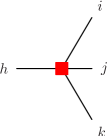
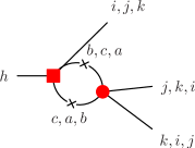
$2i\mathop{\mathrm{Im}}\nolimits\quad$ $\quad=\quad$ $\quad+\quad$

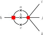
Figure 2: Diagrammatic representation of the unitarity relation in Eq. (26). The crosses indicate on-shell particles and phase space integration.

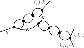
Figure 3: Contribution which is included on the r.h.s. of Eq. (26), but not in $\mathcal{A}$ on the l.h.s. The crosses indicate on-shell particles and phase space integration.

3.2 Isospin decomposition

In order to study the importance of the various two-particle channels in the final state interactions and corresponding contributions from well-known resonances like $f_{0}(980)$, $a_{0}(980)$ we perform a decomposition into isospin channels. Assigning one common mass for all particles of an isospin multiplet this can straightforwardly be done for the isospin-conserving decay modes $\eta^{\prime}\to\eta\pi\pi$. To this aim, we decompose the interaction kernel of the Bethe-Salpeter equation, Eq. (23), into an isospin-conserving and an isospin-breaking part, $\hat{A}_{l}^{\textrm{(ic)}}$ and $\hat{A}_{l}^{\textrm{(ib)}}$, respectively, so that

$$\hat{A}_{l}=O\,\hat{A}_{l}^{\textrm{(ic)}}\,O^{T}+O\,\hat{A}_{l}^{\textrm{(ib)}}\,O^{T}\ ,$$ (29)

where $O$ represents the orthogonal transformation which transforms from the isospin to the physical basis. Analogous to the definition of $\hat{T}_{l}$ we can construct the unitarized amplitude $\hat{T}_{l}^{\textrm{(ic)}}$ in the isospin limit by replacing $\hat{A}_{l}$ by $\hat{A}_{l}^{\textrm{(ic)}}$ in Eq. (23). After substituting in Eq. (25) the pieces of the form $[\hat{T}_{l}-\hat{A}_{l}]$ by $O[\hat{T}_{l}^{\textrm{(ic)}}-\hat{A}_{l}^{\textrm{(ic)}}]O^{T}$, the influence of the different isospin channels may be examined by omitting one specific combination of isospin and angular momentum quantum numbers.

The situation is slightly more complicated for the isospin-breaking decays of $\eta$ and $\eta^{\prime}$ into three pions. Retaining only one isospin-breaking vertex and inserting it at all possible places in the bubble chain, the decay amplitude in terms of isospin channels is found by replacing in Eq. (25) the pieces of the form $[\hat{T}_{l}-\hat{A}_{l}]$ by

$$O[\hat{T}_{l}^{\textrm{(ic)}}\,\hat{G}_{l}\,\hat{A}_{l}^{\textrm{(ib)}}\,\hat{G}_{l}\,\hat{T}_{l}^{\textrm{(ic)}}-\hat{T}_{l}^{\textrm{(ic)}}\,\hat{G}_{l}\,\hat{A}_{l}^{\textrm{(ib)}}-\hat{A}_{l}^{\textrm{(ib)}}\,\hat{G}_{l}\,\hat{T}_{l}^{\textrm{(ic)}}]O^{T}\ .$$ (30)

While the second and third term in the bracket describe the insertion of the isospin-breaking vertex at both ends of the bubble chain, the first one includes insertions at all intermediate points.

4 Results

We now turn to the discussion of the numerical results of the calculation which are obtained from a combined analysis of the decay widths, branching ratios, and slope parameters of the considered decays as well as phase shifts in meson-meson scattering. The widths of $\eta\to 3\pi$ and $\eta^{\prime}\to\eta\pi\pi$ have been measured roughly at the 10 % precision level, while for $\eta^{\prime}\to 3\pi^{0}$ the experimental uncertainty is considerably larger and only an upper limit exists for $\Gamma(\eta^{\prime}\to\pi^{+}\pi^{-}\pi^{0})$ [11]. Moreover, some of these decay widths are constrained by the well-measured branching ratios

$$r_{1}=\frac{\Gamma(\eta\to 3\pi^{0})}{\Gamma(\eta\to\pi^{+}\pi^{-}\pi^{0})}\,,\qquad r_{2}=\frac{\Gamma(\eta^{\prime}\to 3\pi^{0})}{\Gamma(\eta^{\prime}\to\eta\pi^{0}\pi^{0})}\,.$$ (31)

The Dalitz plot distribution of the decay $h\to i\,j\,k$ (with $j=\bar{k}$) is conventionally described in terms of the two variables

$$x = \frac{\sqrt{3}(u-t)}{2m_{h}(m_{h}-m_{i}-2m_{jk})}\ ,$$

$$y = \frac{(m_{i}+2m_{jk})\big{[}(m_{h}-m_{i})^{2}-s\big{]}}{2m_{h}m_{jk}(m_{h}-m_{i}-2m_{jk})}-1\ ,$$ (32)

where the $m_{x}$ denote the masses of the respective particles ($m_{j}=m_{k}=m_{jk}$) and the Mandelstam variables have been defined in Eq. (24). In $\eta\to 3\pi$ measurements (e.g. [24]) a slightly simpler definition of $y$, where $(m_{\pi^{0}}+2m_{\pi^{+}})/m_{\pi^{+}}$ is replaced by 3, is usually employed,

$$y=\frac{3\big{[}(m_{h}-m_{i})^{2}-s\big{]}}{2m_{h}(m_{h}-m_{i}-2m_{jk})}-1\ ,$$ (33)

but the difference is at the level of 1 % and can be safely neglected. The squared absolute value of the amplitude, $|\mathcal{A}_{hijk}(x,y)|^{2}$, is then expanded for $\eta^{\prime}\to\eta\pi\pi$ and the charged decay modes of $\eta,\eta^{\prime}\to 3\pi$ as

$$|\mathcal{A}(x,y)|^{2}=|N|^{2}\big{[}1+ay+by^{2}+cx^{2}+dy^{3}+\cdots\big{]}\,,$$ (34)

while for the decays into three identical particles Bose symmetry dictates the form

$$|\mathcal{A}(x,y)|^{2}=|N^{\prime}|^{2}\big{[}1+g(y^{2}+x^{2})+\cdots\big{]}\,.$$ (35)

For the Dalitz plot parameters $a$, $b$, $c$ of $\eta\to\pi^{+}\pi^{-}\pi^{0}$ the experimental situation is not without controversy. We employ the numbers of [24], since it is the most recent published measurement and the results appear to be consistent with the bulk of the other experiments listed by the Particle Data Group [11]. They differ somewhat from the new preliminary results of the KLOE Collaboration [9] that has found a non-zero value for the third order parameter $d$ which was not included in previous experimental parametrizations. Very recently the Dalitz plot parameters of $\eta^{\prime}\to\eta\pi^{+}\pi^{-}$ have been determined with high statistics by the VES experiment [10]. While we will employ in our fits the experimental Dalitz parameters provided by the Particle Data Group [11], we will also discuss further below the modifications of our results when the two new and precise (but so far preliminary) data sets [9, 10] are taken into account. Note that the slope parameters of $\eta^{\prime}\to 3\pi$ have not yet been determined experimentally, but such a measurement is intended at WASA@COSY [12].

From the unitarized partial-wave $T$-matrix in Eq. (17) one may also derive the phase shifts in meson-meson scattering. Hence, our approach is further constrained by the experimental phase shifts for $\pi\pi\to\pi\pi,K\bar{K}$ scattering. The results of the fit are presented in Appendix B.

The coupled-channels framework entails several parameters, i.e. the low-energy constants (LECs) of the chiral effective Lagrangian up to fourth order and the subtraction constants $a_{m\bar{m}}$ in the loop integrals $G_{m\bar{m}}$ which are embodied in the coupled-channels $T$-matrix. It turns out that only the fit to the $\pi\pi$ phase shifts in the $I=J=1$ channel (which includes the $\rho$ resonance) requires a non-zero value of the corresponding subtraction constant $a_{\pi\pi}^{(I=J=1)}(\mu)$. The regularization scale of $G_{m\bar{m}}$ is set to $\mu=1$ GeV for all channels. As a guiding principle for the importance of the LECs and in order to reduce their number, we make use of large-$N_{c}$ arguments in the effective Lagrangian and set all LECs to zero which are of order $\mathcal{O}(1/N_{c}^{2})$ and thus suppressed by at least three powers of $1/N_{c}$ with respect to the leading coefficients. Their effects are expected to be small and can be partially compensated by readjusting the leading and subleading coefficients in our fits. Furthermore, we set those parameters to zero by hand which turn out to be less sensitive to the processes under consideration. It turns out, that with the exception of $v_{1}^{(2)}$ and $\beta_{14}^{(0)}$ all parameters of order $\mathcal{O}(1/N_{c})$ have a negligible effect when varying them within small ranges around zero and can be safely neglected. To summarize, we only keep the LECs

$$\begin{array}[]{c}\beta_{0}^{(0)},\,\beta_{3}^{(0)},\,\beta_{5}^{(0)},\,\beta_{8}^{(0)}=\mathcal{O}(N_{c})\,,\\[6.45831pt] v_{0}^{(2)},\,v_{3}^{(1)},\,\beta_{1}^{(0)},\,\beta_{2}^{(0)},\,\beta_{4}^{(0)},\,\beta_{6}^{(0)},\,\beta_{7}^{(0)},\,\beta_{13}^{(0)},\,\beta_{18}^{(0)},\,=\mathcal{O}(1)\,,\\[6.45831pt] v_{1}^{(2)},\,\beta_{14}^{(0)}=\mathcal{O}(1/N_{c})\,.\end{array}$$ (36)

The coefficient $v_{0}^{(2)}$ is related to the mass of the $\eta^{\prime}$ in the chiral limit, $m_{0}$, and has been constrained to the range $0.00183\,\mathrm{GeV}^{4}\dots 0.00523\,\mathrm{GeV}^{4}$ in [18], while the rest of the parameters of order $\mathcal{O}(N_{c}^{i})$ may be varied within small ranges around zero, naturally given by $\pm N_{c}^{i}f^{2}/(12\Lambda_{\chi}^{n})$, where $n$ depends on the dimension of the constant under consideration. In conventional ChPT the $\beta_{0}$ term is usually not listed, since it can be absorbed into other contact terms by virtue of a Cayley-Hamilton matrix identity. However, this transformation mixes different orders in $1/N_{c}$, hence we prefer to keep this term explicitly, in order to retain the clean large $N_{c}$ behavior of the $\beta_{i}$’s.

By fitting to all available (published) data sets of the investigated hadronic $\eta,\eta^{\prime}$ decays and the phase shifts an overall $\chi^{2}$ function is calculated. To this end, we compute $\chi^{2}$ values for all observables i.e. phase shifts, decay widths, branching ratios and Dalitz plot parametrizations, divide them by the number of experimental data points and take the sum afterwards. In order to find the minima of the overall $\chi^{2}$ function, we perform a random walk in parameter space, where only steps which lead to a smaller $\chi^{2}$ value are allowed, and a very large number of random walks with randomized starting points is carried out. We observe four different classes of fits which are all in very good agreement with the currently available (published) data on hadronic decays, but differ in the description of the decays $\eta^{\prime}\to 3\pi$ where experimental constraints are scarce.

The errors which we specify in the following for all parameters and observables reflect the deviations which arise when we allow for $\chi^{2}$ values which are at most 15 % larger than the minimum value. Although this choice is somewhat arbitrary, it illustrates how variation of the $\chi^{2}$ function in parameter space affects the results.

4.1 $\eta\to 3\pi$

The results for the decays $\eta\to 3\pi$, which agree very well with the experimental values, are shown in Table 1. Most remarkably our approach is able to reproduce the new, precise value of the $\eta\to 3\pi^{0}$ Dalitz parameter $g$ measured by the Crystal Ball Collaboration [25] (and prevailing the PDG average value [11]) which could not be met in previous investigations [5, 8]. With regard to [8] this is mainly due to the larger number of chiral parameters taken into account in the present work and the improved fitting routine utilized. The PDG number for $g$ does, however, not agree with the preliminary $g$ value of the KLOE Collaboration [9] which comes close to the results given in [5, 8]. The detailed discussion of the new KLOE results for the Dalitz plot distributions of $\eta\to\pi^{+}\pi^{-}\pi^{0}$ and $\eta\to 3\pi^{0}$ is deferred to Secs. 4.5 and 5.

When electromagnetic effects are neglected (which is justified according to Sutherland’s theorem [1]), the isospin-violating decay of $\eta$ into three pions can only take place via a finite quark mass difference $m_{u}-m_{d}$. The decay amplitude is therefore proportional to $m_{\epsilon}^{2}$ defined in Eq. (4) and we have employed the value which follows from Dashen’s theorem, Eq. (5) [17]. Deviations of the calculated decay widths from the measured numbers could thus be interpreted as a hint to non-negligible subleading corrections to the leading order result by Dashen. In order to quantify these deviations, one commonly defines the double quark mass ratio

$$Q^{2}=\frac{m_{s}-\hat{m}}{m_{d}-m_{u}}\frac{m_{s}+\hat{m}}{m_{d}+m_{u}}\ ,$$ (37)

and Dashen’s theorem yields $Q_{\textrm{Dashen}}=24.1$. Differing $Q$-values lead to decay widths which are related to the original one, $\Gamma_{\textrm{Dashen}}$, by

$$\Gamma=\left(\frac{Q_{\textrm{Dashen}}}{Q}\right)^{4}\Gamma_{\textrm{Dashen}}\ .$$ (38)

Taking into account theoretical as well as experimental uncertainties we find from a comparison of our results with data $Q=24.0\pm 0.6$ which is consistent with the result of [8]. Note, however, that this obvious agreement with Dashen’s theorem merely reflects the fact that our approach is capable of reproducing the experimental decay widths of $\eta\to 3\pi$. Due to the larger number of chiral parameters with increased ranges compared to [8] and the improved fitting procedure we can easily compensate the effects from variations in $Q$ by readjusting the chiral parameters of our approach. We have checked that variations of $Q$ in the range of $20\dots 24$ which covers the various (and partially contradictory) results in the literature [26] can be accommodated within this approach. Therefore, our analysis does not allow for conclusions on the size of the violation of Dashen’s theorem.

Extending the work of [8] we have also taken $p$-wave final state interactions into account. By setting these contributions to zero, we find that the decay width of $\eta\to\pi^{+}\pi^{-}\pi^{0}$ is reduced by a tiny fraction of 0.7 % implying rapid convergence of the partial wave expansion. The Dalitz plot parameters, which are more sensitive to the precise form of the amplitude than the width, are also only moderately altered. Without $p$-waves we obtain $a=-1.15\pm 0.07$, $b=0.29\pm 0.05$, $c=0.01\pm 0.02$. Note that due to Bose symmetry there is no $p$-wave contribution to the decay into three neutral pions.

Certainly, the most important isospin channel for final state interactions in $\eta\to 3\pi$ is the $I=0$ $s$-wave rescattering which is dominated by $\pi\pi$ interactions. Omitting this channel reduces the decay width by 73 %. The other two $s$-wave channels with isospin one and two, respectively, interfere destructively with the former. To be more precise, taking out the $I=1$ part, which mainly reflects $\pi\eta$ interactions, enlarges the decay width of $\eta\to\pi^{+}\pi^{-}\pi^{0}$ ($\eta\to 3\pi^{0}$) by 9 % (10 %), while setting the $I=2$ channel, which is purely $\pi\pi$ rescattering, to zero results in an enhancement of the decay widths by 16 % (20 %). The only relevant $p$-wave contributions arise from the $I=1$ channels $\pi\eta$, $\pi\eta^{\prime}$ which are $C$-even and thus do not couple to $C$-odd channels related to the $\rho(770)$ resonance. Neglecting the $I=J=1$ channels reduces the $\eta\to\pi^{+}\pi^{-}\pi^{0}$ decay width by roughly 1 %. The numerical difference to the statement on the importance of $p$-wave contributions in the previous paragraph is due to the fact that for the decomposition into isospin channels we use isospin-symmetrized masses, while otherwise we employ the physical values of the masses.

Finally, we have also examined to which extent the amplitude violates three-particle unitarity in the spectator approximation as described in Sec. 3.1. In order to quantify the violation of Eq. (27), we compute the absolute value of the difference between l.h.s. and r.h.s. normalized by the modulus of the amplitude $\mathcal{A}_{hijk}$. Averaged over the whole Dalitz plot we find this violation to be $(2.5\pm 0.3)\,\%$ for the process $\eta\to\pi^{+}\pi^{-}\pi^{0}$ and—even smaller—$(1.3\pm 0.3)\,\%$ for the decay into three neutral pions. The fact that the violation of Eq. (27) is so small is non-trivial since only two-body unitarity, but not three-body unitarity is implemented in the definition of the decay amplitude. This may suggest that three-body effects (like multiple scattering of one particle in the final state with the other two or a genuine three-body interaction) are of the same order of magnitude. A more detailed investigation of this issue will be the subject of future work [23].

	$\Gamma_{\eta\to 3\pi^{0}}$ (eV)	$\Gamma_{\eta\to\pi^{+}\pi^{-}\pi^{0}}$ (eV)	$r_{1}$
theo.	$422\,\pm\,13$	$290\,\pm\,8$	$1.46\,\pm\,0.02$
exp.	$419\,\pm\,27$	$292\,\pm\,21$	$1.44\,\pm\,0.04$
	$a$	$b$	$c$	$g$
theo.	$-1.20\,\pm\,0.07$	$0.28\,\pm\,0.05$	$0.05\,\pm\,0.02$	$-0.062\,\pm\,0.006$
exp.	$-1.22\,\pm\,0.07$	$0.22\,\pm\,0.11$	$0.06\,\pm\,0.02$	$-0.062\,\pm\,0.008$

Table 1: Results for the partial decay widths of $\eta\to 3\pi$, the branching ratio $r_{1}$, and the Dalitz plot parameters compared to experimental data from [11] and [24].

4.2 $\eta^{\prime}\to 3\pi$

Only sparse experimental information exists on the decays of $\eta^{\prime}$ into three pions. The experimental decay width of $\eta^{\prime}\to 3\pi^{0}$ is [11]

$$\Gamma^{\textrm{(exp)}}(\eta^{\prime}\to 3\pi^{0})=(315\pm 78)\,\mathrm{eV}$$ (39)

which is nicely met within our approach:

$$\Gamma^{\textrm{(theo)}}(\eta^{\prime}\to 3\pi^{0})=(330\pm 33)\,\mathrm{eV}\,.$$ (40)

For the decay into $\pi^{+}\pi^{-}\pi^{0}$ only a weak experimental upper limit exists [11]

$$\Gamma^{\textrm{(exp)}}(\eta^{\prime}\to\pi^{+}\pi^{-}\pi^{0})<10\,\mathrm{keV}\,.$$ (41)

Due to the large phase space available in these two decay modes of the $\eta^{\prime}$, final state interactions are expected to be of greater importance. Indeed we find that in contrast to the processes $\eta\to 3\pi$ and $\eta^{\prime}\to\eta\pi\pi$ the Dalitz plot distribution of $\eta^{\prime}\to 3\pi$—depending on the choice of the chiral parameters—cannot always be well parametrized by a simple second or third order polynomial in $x$ and $y$. Nevertheless, it happens that all our fits may be classified into four groups mainly due to the different values of the lower order coefficients in $x$ and $y$. The numerical results for these most relevant coefficients are compiled in Tables 2 and 3 along with the predicted width of $\eta^{\prime}\to\pi^{+}\pi^{-}\pi^{0}$ and the order of the polynomial in $x$ and $y$ which is needed to obtain a reasonable approximation to the Dalitz plot distribution resulting from our approach. Note that due to charge conjugation invariance, only even powers of $x$ appear. Examples of two very different Dalitz plots are shown in Fig. 4. Despite these differing predictions one should keep in mind that all fits describe all available experimental data at the same level of accuracy. The Dalitz plot distributions of these decays pose therefore tight constraints for our approach and must be compared with future experiments at the WASA@COSY facility.

			cluster 1	cluster 2	cluster 3	cluster 4
$\Gamma_{\eta^{\prime}\to\pi^{+}\pi^{-}\pi^{0}}$ (eV)			$470\,\pm\,200$	$520\,\pm\,200$	$740\,\pm\,420$	$620\,\pm\,180$
coeff.	$y$	(“$a$”)	$0.6\,\pm\,5.2$	$2.4\,\pm\,1.7$	$0.3\,\pm\,1.1$	$4.4\,\pm\,1.2$
coeff.	$y^{2}$	(“$b$”)	$10.0\,\pm\,11.0$	$2.1\,\pm\,7.5$	$-5.2\,\pm\,1.5$	$14.9\,\pm\,6.7$
coeff.	$x^{2}$	(“$c$”)	$0.1\,\pm\,3.6$	$-0.7\,\pm\,1.4$	$0.1\,\pm\,1.6$	$-3.7\,\pm\,1.5$
coeff.	$y^{3}$	(“$d$”)	$-6.1\,\pm\,11.5$	$-0.6\,\pm\,14.0$	$-8.8\,\pm\,7.8$	$27.5\,\pm\,18.1$
coeff.	$x^{2}y$		$-10.8\,\pm\,11.2$	$2.0\,\pm\,3.0$	$-7.4\,\pm\,5.6$	$-1.5\,\pm\,2.8$
coeff.	$y^{4}$		$0.6\,\pm\,12.2$	$-3.2\,\pm\,7.3$	$23.3\,\pm\,20.7$	$24.5\,\pm\,11.6$
coeff.	$x^{2}y^{2}$		$13.9\,\pm\,23.6$	$11.8\,\pm\,22.4$	$-17.7\,\pm\,9.4$	$39.0\,\pm\,12.7$
coeff.	$x^{4}$		$-0.5\,\pm\,11.5$	$-1.2\,\pm\,16.1$	$15.4\,\pm\,9.8$	$-20.5\,\pm\,9.4$
poly. order			6 – 8	4 – 8	$\geq 8$	$\geq 8$

Table 2: Results for the decay width of $\eta^{\prime}\to\pi^{+}\pi^{-}\pi^{0}$ and the leading Dalitz plot parameters. The last line denotes the order of the polynomial which is needed to describe the Dalitz plot distribution.

			cluster 1	cluster 2	cluster 3	cluster 4
coeff.	$x^{2}$, $y^{2}$	(“$g$”)	$0.1\,\pm\,1.7$	$-2.7\,\pm\,1.0$	$-2.1\,\pm\,0.7$	$-0.2\,\pm\,0.6$
coeff.	$y^{3}$		$-0.5\,\pm\,1.4$	$-1.7\,\pm\,0.7$	$-0.2\,\pm\,0.6$	$-0.8\,\pm\,0.6$
coeff.	$x^{2}y$		$1.6\,\pm\,4.1$	$5.0\,\pm\,1.9$	$0.6\,\pm\,1.8$	$2.3\,\pm\,1.7$
coeff.	$y^{4}$		$0.2\,\pm\,1.4$	$2.6\,\pm\,1.5$	$1.6\,\pm\,0.8$	$-0.1\,\pm\,1.1$
coeff.	$x^{2}y^{2}$		$0.4\,\pm\,2.9$	$5.3\,\pm\,2.8$	$3.5\,\pm\,1.7$	$0.2\,\pm\,2.5$
coeff.	$x^{4}$		$0.1\,\pm\,1.5$	$2.7\,\pm\,1.5$	$1.7\,\pm\,0.9$	$0.1\,\pm\,1.2$
poly. order			3 – 6	5 – 6	4 – 6	3 – 5

Table 3: Results for the leading Dalitz plot parameters of $\eta^{\prime}\to 3\pi^{0}$. The last line denotes the order of the polynomial which is needed to describe the Dalitz plot distribution.

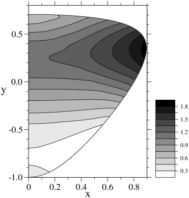
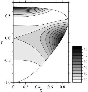
(a)		(b)

Figure 4: Sample $\eta^{\prime}\to\pi^{+}\pi^{-}\pi^{0}$ Dalitz plot distribution $|\mathcal{A}(x,y)/\mathcal{A}(0,0)|^{2}$ of cluster 2 which can be described by a fourth order polynomial in $x$ and $y$ (a) and of cluster 3 which must be parametrized by a polynomial of eighth order (b). Due to their symmetry under $x\to-x$ only the right half of the Dalitz plots is shown.

While in $\eta^{\prime}\to 3\pi^{0}$ $p$-wave contributions in two-body rescattering are forbidden by Bose symmetry, they can be large in $\eta^{\prime}\to\pi^{+}\pi^{-}\pi^{0}$ due to large phase space. Interestingly, their size varies significantly depending on the cluster of fit parameters. They are largest for the fits of cluster 4 where setting them to zero diminishes the decay width by 50 % on average. The partial width is reduced by 44 % (28 %) for cluster 3 (cluster 1), while for the parameter sets of cluster 2 suppressing the $p$-wave contributions alters the width by less than 10 %. The large higher order coefficients of the $\eta^{\prime}\to\pi^{+}\pi^{-}\pi^{0}$ Dalitz plot distribution are mainly due to $p$-wave contributions. If $p$-waves are omitted, the fits of clusters 3 and 4 can be well parametrized by polynomials of fifth order in $x$ and $y$, while for most fits in clusters 1 and 2 a sixth order polynomial would be sufficient, cf. Table 2. Note that in analogy to the decay $\eta\to 3\pi$ $p$-wave final state interactions with the quantum numbers of the $\rho(770)$ meson do not occur.

In $\eta^{\prime}\to 3\pi$ the contributions from the various isospin channels depend sensitively on the cluster, e.g., omitting the $I=J=0$ channel in $\eta^{\prime}\to 3\pi^{0}$ reduces the decay width by 84 % for cluster 1, while it is enhanced by 132 % on average for the fits of cluster 3. For brevity we refrain from giving the full list of isospin contributions.

4.3 $\eta^{\prime}\to\eta\pi\pi$

In Tables 4 and 5 we show the results for the dominant hadronic decay modes of the $\eta^{\prime}$, namely the decays into $\eta\pi^{+}\pi^{-}$ and $\eta\pi^{0}\pi^{0}$. They are all in very good agreement with the existing (and published) experimental data. Furthermore, we have calculated the branching ratio $r_{2}$, Eq. (31), which links the two neutral decay modes $\eta^{\prime}\to 3\pi^{0}$ and $\eta^{\prime}\to\eta\pi^{0}\pi^{0}$. We find

$$r_{2}^{\textrm{(theo)}}=(71\pm 7)\times 10^{-4},\qquad r_{2}^{\textrm{(exp)}}=(74\pm 12)\times 10^{-4}\quad\mbox{\cite[cite]{[\@@bibref{}{pdg}{}{}]}},$$ (42)

and the accordance with experiment is again persuasive.

In the isospin limit, $m_{u}=m_{d}$, the decay width $\Gamma(\eta^{\prime}\to\eta\pi^{+}\pi^{-})$ would be exactly given by 2 $\Gamma(\eta^{\prime}\to\eta\pi^{0}\pi^{0})$, due to the symmetry factor for identical particles in the latter process. If, however, one is interested in the isospin-breaking contributions in the amplitude of $\eta^{\prime}\to\eta\pi\pi$, one ought to disentangle it from phase space effects which are caused by the different masses of charged and neutral pions. With an isospin-symmetric decay amplitude, but physical masses in the phase space factors, we find a ratio

$$r_{3}=\frac{\Gamma(\eta^{\prime}\to\eta\pi^{+}\pi^{-})}{\Gamma(\eta^{\prime}\to\eta\pi^{0}\pi^{0})}=1.78\pm 0.02\,,$$ (43)

which is smaller than 2 and compares to $r_{3}=1.77\pm 0.02$ when isospin-breaking is taken into account in the amplitude. (For comparison, if the amplitude is set constant and the physical pion masses are employed in the phase space integrals, the ratio is given by $r_{3}=1.77$.) We may thus conclude that within our approach isospin-breaking corrections in the $\eta^{\prime}\to\eta\pi\pi$ decay amplitude are tiny. The branching ratio $r_{3}$ has not been measured directly. If, however, we calculate the ratio of fractions $\Gamma_{i}/\Gamma_{\textrm{total}}$ for these two decay modes using the numbers and correlation coefficients published by the Particle Data Group [11], we arrive at

$$r_{3}^{\textrm{(exp)}}=2.12\pm 0.19$$ (44)

by means of standard error propagation. Such a large branching ratio would indicate significant isospin-violating contributions in the amplitude. But the experimental uncertainties are sizable and should be reduced by the upcoming experiments with WASA at COSY [12] and at MAMI-C [13].

	$\Gamma_{\eta^{\prime}\to\eta\pi^{+}\pi^{-}}$			$a$		$b$		$c$
theo.	$81$$\,\pm\,$	$4$	keV	$-0.116$$\,\pm\,$	$0.024$	$0.000$$\,\pm\,$	$0.019$	$0.016$$\,\pm\,$	$0.035$
exp.	$89$$\,\pm\,$	$11$	keV	$-0.16$$\,\pm\,$	$0.06$

Table 4: Results for the partial decay width of $\eta^{\prime}\to\eta\pi^{+}\pi^{-}$ and the Dalitz plot parameters compared to experimental data from [11].

	$\Gamma_{\eta^{\prime}\to\eta\pi^{0}\pi^{0}}$			$a$		$b$		$c$
theo.	$46$$\,\pm\,$	$3$	keV	$-0.122$$\,\pm\,$	$0.025$	$0.003$$\,\pm\,$	$0.018$	$0.019$$\,\pm\,$	$0.039$
exp.	$42$$\,\pm\,$	$6$	keV	$-0.116$$\,\pm\,$	$0.026$	$0.003$$\,\pm\,$	$0.017$	$0.00$$\,\pm\,$	$0.03$

Table 5: Results for the partial decay width of $\eta^{\prime}\to\eta\pi^{0}\pi^{0}$ and the Dalitz plot parameters compared to experimental data from [11].

It turns out that $p$-wave final state interactions are tiny in the processes $\eta^{\prime}\to\eta\pi\pi$. The corrections to the decay widths which they generate are smaller than 0.02 % and can thus be safely neglected. Consequently, in the isospin basis the relevant two-body channels are given by $s$-wave interactions of isospin 0 or 1 states. When examining the influence of these two channels on the $\eta^{\prime}\to\eta\pi\pi$ partial widths we observe an interesting pattern. By setting the $I=0$ channel to zero for the fits of cluster 1 (cluster 2) the widths are lowered by 22 % (22 %), while suppressing the $I=1$ part reduces them by 81 % (72 %). When the fit parameters of clusters 1 and 2 are employed, the isospin one channel which includes the tail of the $a_{0}(980)$ resonance thus appears to be of great importance for the decay mode $\eta^{\prime}\to\eta\pi\pi$ confirming the findings of [8] and [6]. The situation is, however, reversed if one considers the fits of the remaining two clusters. Taking out the $I=0$ channel in the final state interactions of the fits of cluster 3 (cluster 4) diminishes the decay widths by 79 % (81 %), whereas erasing the channel with $I=1$ reduces it by only 33 % (28 %). Accordingly, for these sets of parameters the $I=0$ channel, which incorporates the effects of the $f_{0}(980)$ resonance and the $\pi\pi$ correlation at lower energies, has higher impact on the decay widths than the $a_{0}(980)$ channel. Although the fits of all four clusters yield very similar results for all $\eta^{\prime}\to\eta\pi\pi$ observables, the two scenarios can be distinguished by their correlation with the processes $\eta^{\prime}\to 3\pi$ provided within our approach. Thus, a precise measurement of $\eta^{\prime}\to 3\pi$ decay parameters can also help to clarify the importance of $a_{0}(980)$ or $f_{0}(980)$ resonance contributions to the dominant decay mode of the $\eta^{\prime}$ into $\eta\pi\pi$.

The violation of three-particle unitarity as described in Sec. 3.1 is not as tiny as in the case of $\eta\to 3\pi$, but still remarkably small. Using the definition of Sec. 4.1 we find averaged deviations of $(11\pm 7)\,\%$ for $\eta^{\prime}\to\eta\pi^{+}\pi^{-}$ and $(10\pm 6)\,\%$ for $\eta^{\prime}\to\eta\pi^{0}\pi^{0}$. It remains to be seen whether corrections from other three-body effects which are not included in the approach will be of comparable size [23].

4.4 Numerical values of the chiral parameters and $\eta$-$\eta^{\prime}$ mixing

Before presenting numerical results for the chiral parameters we would like to stress that the values of the couplings of the effective Lagrangian employed in the coupled-channels approach are in general not identical to those in the perturbative framework. First, contributions from tadpoles (which include also effects from the so-called on-shell approximation), and $t$-/$u$-channel diagrams in the interaction kernel have been absorbed into the coupling constants. Second, the BSE summarizes meson-meson scattering in the $s$-channel to infinite order. The contributions beyond a given chiral order are missing in the perturbative approach and lead to changes in the values of the couplings when fitting the results to data. Finally, the subtraction point in the renormalization procedure can be different in both schemes. Hence, one must expect differences in the values of the coupling constants utilized in both frameworks.

In Table 6 we show the numerical values of the low-energy constants as well as the non-zero subtraction constant $a_{\pi\pi}^{(I=J=1)}$ as they come out for the fits of the four different clusters. In addition we display the parameters of $\eta$-$\eta^{\prime}$ mixing $R_{0\eta}$, $R_{8\eta^{\prime}}$ which are determined by the values of the LECs $v_{3}^{(1)}$, $\beta_{5}^{(0)}$, and $\beta_{18}^{(0)}$ in virtue of Eq. (8). Note that compared to the analysis in [8] we have increased the number of chiral parameters which—in conjunction with an improved fitting procedure—helped to considerably improve the agreement with experimental data on hadronic $\eta$, $\eta^{\prime}$ decays.

According to the mixing parameters the four clusters of fits may be divided into two groups. For clusters 1 and 2 $R_{0\eta}$ and $R_{8\eta^{\prime}}$ are both of similar small size and (mainly) positive, while clusters 3 and 4 feature a large, positive $R_{0\eta}$ and an $R_{8\eta^{\prime}}$ which is close to zero. Within the present analysis the second mixing parameter $R_{8\eta^{\prime}}$, which characterizes the fraction of the pure octet field $\eta_{8}$ in the physical $\eta^{\prime}$, turns out to be more tightly constrained by the fit than $R_{0\eta}$ which describes the singlet content of the $\eta$. In all cases the numerical results for $R_{0\eta}$ and $R_{8\eta^{\prime}}$ deviate sizably from an orthogonal mixing scheme, where $R_{0\eta}=-R_{8\eta^{\prime}}$. For comparison, a mixing angle of $-20^{\circ}$ in the one-mixing angle scheme as found in the literature [3] would correspond to $R_{0\eta}=-R_{8\eta^{\prime}}=0.34$.

The fitting procedure does not constrain all parameters at the same level of accuracy. While some (e.g. $v_{3}^{(1)}$, $\beta_{3}^{(0)}$, $\beta_{5}^{(0)}$, $\beta_{8}^{(0)}$, $\beta_{18}^{(0)}$) may vary within large ranges (partly compensating each other), others like $v_{0}^{(2)}$, $\beta_{0}^{(0)}$, $\beta_{1}^{(0)}$, $\beta_{2}^{(0)}$, and $\beta_{4}^{(0)}$ are relatively tightly fixed. These boundaries constitute important constraints which must be met in future coupled-channels analyses of mesonic processes within the approach described here. In particular, the coefficient $v_{0}^{(2)}$ encodes the mass of the $\eta^{\prime}$ in the chiral limit, $m_{0}$, by virtue of

$$m_{0}^{2}=\frac{2v_{0}^{(2)}}{f^{2}}\,.$$ (45)

The fact that the $\eta^{\prime}$ does not become massless in the chiral limit is a consequence of the axial U(1) anomaly of QCD which generates in the divergence of the singlet axial-vector current an additional, non-vanishing term involving the gluonic field strength tensor. In the effective theory this term is represented by $v_{0}^{(2)}$. Employing $f=88\,\mathrm{MeV}$, the value of the pseudoscalar decay constant in the chiral limit [27], we find from the fits of all clusters $m_{0}=(900\pm 80)\,\mathrm{MeV}$ which is close to the physical mass of the $\eta^{\prime}$.

		cluster 1	cluster 2	cluster 3	cluster 4
$v_{3}^{(1)}$	$\times 10^{3}\,\mathrm{GeV}^{-2}$	$0.82\,\pm\,1.65$	$0.23\,\pm\,1.46$	$-1.92\,\pm\,0.62$	$-1.47\,\pm\,0.83$
$v_{0}^{(2)}$	$\times 10^{3}\,\mathrm{GeV}^{-4}$	$3.15\,\pm\,0.39$	$3.21\,\pm\,0.49$	$3.07\,\pm\,0.42$	$2.89\,\pm\,0.30$
$v_{1}^{(2)}$	$\times 10^{3}\,\mathrm{GeV}^{-2}$	$-0.16\,\pm\,0.34$	$-0.12\,\pm\,0.32$	$-0.07\,\pm\,0.17$	$-0.13\,\pm\,0.13$
$\beta_{0}^{(0)}$	$\times 10^{3}$	$-0.12\,\pm\,0.18$	$-0.07\,\pm\,0.22$	$-0.06\,\pm\,0.19$	$-0.02\,\pm\,0.32$
$\beta_{1}^{(0)}$	$\times 10^{3}$	$-0.47\,\pm\,0.25$	$-0.57\,\pm\,0.22$	$-0.49\,\pm\,0.14$	$-0.49\,\pm\,0.18$
$\beta_{2}^{(0)}$	$\times 10^{3}$	$0.77\,\pm\,0.18$	$0.72\,\pm\,0.23$	$0.69\,\pm\,0.19$	$0.64\,\pm\,0.34$
$\beta_{3}^{(0)}$	$\times 10^{3}$	$0.05\,\pm\,0.55$	$0.19\,\pm\,0.51$	$0.06\,\pm\,0.26$	$0.11\,\pm\,0.15$
$\beta_{4}^{(0)}$	$\times 10^{3}$	$0.33\,\pm\,0.18$	$0.34\,\pm\,0.15$	$0.39\,\pm\,0.12$	$0.42\,\pm\,0.14$
$\beta_{5}^{(0)}$	$\times 10^{3}$	$0.73\,\pm\,0.62$	$0.86\,\pm\,0.66$	$0.77\,\pm\,0.83$	$0.48\,\pm\,0.22$
$\beta_{6}^{(0)}$	$\times 10^{3}$	$0.00\,\pm\,0.30$	$0.06\,\pm\,0.28$	$-0.25\,\pm\,0.13$	$-0.34\,\pm\,0.15$
$\beta_{7}^{(0)}$	$\times 10^{3}$	$0.13\,\pm\,0.25$	$0.42\,\pm\,0.33$	$1.01\,\pm\,0.49$	$0.76\,\pm\,0.48$
$\beta_{8}^{(0)}$	$\times 10^{3}$	$-0.06\,\pm\,0.41$	$-0.38\,\pm\,0.46$	$0.02\,\pm\,0.51$	$0.15\,\pm\,0.14$
$\beta_{13}^{(0)}$	$\times 10^{3}$	$-0.08\,\pm\,0.65$	$-0.02\,\pm\,0.60$	$0.16\,\pm\,0.42$	$0.23\,\pm\,0.17$
$\beta_{14}^{(0)}$	$\times 10^{3}$	$0.08\,\pm\,0.35$	$-0.03\,\pm\,0.31$	$-0.21\,\pm\,0.22$	$-0.25\,\pm\,0.14$
$\beta_{18}^{(0)}$	$\times 10^{3}$	$0.80\,\pm\,0.80$	$0.99\,\pm\,0.82$	$1.51\,\pm\,0.47$	$1.49\,\pm\,0.30$
$a_{\pi\pi}^{I=J=1}$	$\times 10^{2}$	$-6.1\,\pm\,0.3$	$-6.1\,\pm\,0.2$	$-6.1\,\pm\,0.3$	$-6.0\,\pm\,0.2$
$R_{0\eta}$		$0.13\,\pm\,0.26$	$0.24\,\pm\,0.23$	$0.61\,\pm\,0.13$	$0.55\,\pm\,0.17$
$R_{8\eta^{\prime}}$		$0.22\,\pm\,0.11$	$0.20\,\pm\,0.08$	$-0.01\,\pm\,0.11$	$-0.04\,\pm\,0.08$

Table 6: Numerical values of the fit parameters itemized according to the four different clusters of fits. They also determine the two $\eta$-$\eta^{\prime}$ mixing parameters $R_{0\eta}$ and $R_{8\eta^{\prime}}$. The regularization scale in $G$ is set to $\mu=1$ GeV.

4.5 Recent experimental developments

Very recently the Dalitz plot distributions of the decays $\eta\to 3\pi$ and $\eta^{\prime}\to\eta\pi^{+}\pi^{-}$ have been determined experimentally with high statistics by the KLOE [9] and the VES Collaboration [10], respectively. In this section we will discuss the changes of our results when these new and precise (though not yet published) data are included in the fit instead of the PDG values. In Table 7 we show the results of a fit, where the VES numbers are taken into account. Since the amplitudes for $\eta^{\prime}\to\eta\pi^{+}\pi^{-}$ and $\eta^{\prime}\to\eta\pi^{0}\pi^{0}$ would be equal in the isospin limit and deviations are thus isospin-breaking and small in our approach, we only include the leading Dalitz parameter $a$ of $\eta^{\prime}\to\eta\pi^{0}\pi^{0}$ and omit the higher ones which are—assuming only small isospin-violating contributions—not quite compatible with the new results of the VES experiment for $\eta^{\prime}\to\eta\pi^{+}\pi^{-}$. Within our approach the $c$ value has a tendency to remain on the positive side in contrast to the result of the VES Collaboration, nevertheless our results are in reasonable overall agreement with the Dalitz plot parameters extracted from the VES experiment. Most remarkably, none of the various other observables (decay widths, branching ratios, Dalitz parameters of other decay modes, etc.) is significantly altered when the VES numbers are included in the fit, so that the very good agreement of the results with all published data of hadronic $\eta$ and $\eta^{\prime}$ decays is retained.

$\eta^{\prime}\to\eta\pi^{+}\pi^{-}$
	$a$	$b$	$c$
theo.	$-0.116\,\pm\,0.011$	$-0.042\,\pm\,0.034$	$0.010\,\pm\,0.019$
exp. [10]	$-0.132\,\pm\,0.019$	$-0.108\,\pm\,0.033$	$-0.046\,\pm\,0.022$
$\eta^{\prime}\to\eta\pi^{0}\pi^{0}$
	$a$	$b$	$c$
theo.	$-0.127\,\pm\,0.009$	$-0.049\,\pm\,0.036$	$0.011\,\pm\,0.021$
exp. [11]	$-0.116\,\pm\,0.026$

Table 7: Results for the Dalitz plot parameters of $\eta^{\prime}\to\eta\pi\pi$ when the VES data [10] are included in the fit.

Next, we have replaced the Dalitz plot parameters of $\eta\to\pi^{+}\pi^{-}\pi^{0}$ and $\eta\to 3\pi^{0}$ quoted in Sec. 4.1 by the new and precise results of the KLOE Collaboration [9] omitting again the VES numbers, in order to avoid interference of these two new, but so far unpublished data sets. The results are compiled in Table 8. While it is possible to accommodate the KLOE numbers for the $a$ and $c$ coefficients of the $\eta\to\pi^{+}\pi^{-}\pi^{0}$ Dalitz plot distribution, our results do not agree with $b$ and $d$. In particular, the value of the $y^{2}$-coefficient $b$ differs from the KLOE number, which has been determined very precisely, by more than five standard deviations. Within the given boundaries for the low-energy coefficients of the chiral effective Lagrangian our approach is unable to produce a $b$ value as small as the number advocated by the KLOE Collaboration [9]. Note that such a small value also implies unexpectedly large corrections to the well-known current algebra result $b=a^{2}/4$ [4, 28]. It may indicate that contributions from higher chiral orders of the effective Lagrangian could play a role for this quantity. But the inclusion of such higher orders is beyond the scope of the present investigation and will not be discussed here.

On the other hand, the KLOE result for the leading order coefficient of the $\eta\to 3\pi^{0}$ Dalitz plot, $g$, cannot be met, while our result still remains compatible with the PDG value, $-0.062\pm 0.008$ [11]. Generally, we observe the pattern, that reducing the $b$ value correlates with an enhancement of the modulus of $g$. Finally, fitting to the new KLOE numbers destroys the agreement of the measured branching ratio $r_{1}$, Eq. (31), and our result, which is significantly increased. The accordance of the rest of the calculated observables with experimental data is only marginally affected by including the KLOE results, also the partial decay widths of the two $\eta\to 3\pi$ decay modes which enter $r_{1}$ remain consistent with the—admittedly large—experimental error bars.

In Table 8 we employ the $r_{1}$ value which is determined by the Particle Data Group by performing a $\chi^{2}$-fit using one decay rate and 18 branching ratios (quoted as “our fit” in [11]). The result of the most recent direct measurement of $r_{1}$ [29], however, is a bit larger and has also larger error bars: $r_{1}=1.52\pm 0.12$, where we have added statistical and systematic errors linearly. Employing this number instead of the PDG value slightly improves the fit to the KLOE data, but does not resolve the disagreement with the Dalitz parameters $b$ and $g$. Taking this value for $r_{1}$ we find $a=-1.049\pm 0.025$, $b=0.178\pm 0.019$, $c=0.079\pm 0.028$, $d=0.064\pm 0.012$, $g=-0.056\pm 0.012$, $r_{1}=1.51\pm 0.01$.

We mention in passing that after relaxing the naturalness assumption on the size of the chiral parameters described at the beginning of this section, we have found a second class of fits, which are slightly closer to the results of the KLOE Collaboration for the Dalitz plot of $\eta\to\pi^{+}\pi^{-}\pi^{0}$. Apart from involving unnaturally large values of some of the LECs they entail a $g$ value which is even larger in magnitude than the one of the previous fits, Table 8. Moreover, the agreement with the experimental phase shifts of $\pi\pi$ scattering in the $I=J=0$ channel shown in Fig. 5 is considerably worsened. The branching ratio $r_{1}$, on the other hand, is not altered, cf. Table 8.

$\eta\to\pi^{+}\pi^{-}\pi^{0}$
	$a$ [9]	$b$ [9]	$c$ [9]	$d$ [9]
theo.	$-1.054\,\pm\,0.025$	$0.185\,\pm\,0.015$	$0.079\,\pm\,0.026$	$0.064\,\pm\,0.012$
exp.	$-1.072\,\pm\,0.013$	$0.117\,\pm\,0.012$	$0.047\,\pm\,0.011$	$0.13\,\pm\,0.03$
	$\eta\to 3\pi$
	$g$ [9]	$r_{1}$ [11]
theo.	$-0.058\,\pm\,0.011$	$1.50\,\pm\,0.01$
exp.	$-0.026\,\pm\,0.018$	$1.44\,\pm\,0.04$

Table 8: Results for the Dalitz plot parameters of $\eta\to 3\pi$ and the branching ratio $r_{1}$, Eq. (31), when the KLOE data [9] are included in the fit. For simplicity we have added the statistical and systematic errors specified in [9] linearly and display symmetrized error bars according to the larger value. Note that our coefficients $c$, $d$, and $g$ correspond to $d$, $f$, and $2\alpha$ in [9], respectively.

5 Dalitz plot parameters of $\eta\to 3\pi$

As pointed out in the previous subsection it is not possible to accommodate the new KLOE results for the Dalitz parameters of $\eta\to 3\pi$ together with the measured branching ratio of the two decay modes, $r_{1}$. In this subsection we will present an explanation how all these experimental quantities can be related in a phenomenological way without making use of model-dependent assumptions on the construction of the decay amplitudes.

The main ingredient is the $\Delta I=1$ selection rule which relates the $\eta\to\pi^{+}\pi^{-}\pi^{0}$ decay amplitude $\mathcal{A}$ to the amplitude $\bar{\mathcal{A}}$ for $\eta\to 3\pi^{0}$ [4]

$$\bar{\mathcal{A}}(s,t,u)=\mathcal{A}(s,t,u)+\mathcal{A}(t,u,s)+\mathcal{A}(u,s,t)\,.$$ (46)

This rule is valid up to tiny corrections from QCD (suppressed by $\mathcal{O}(m_{\epsilon}^{2})$) and of electromagnetic origin (suppressed by $\mathcal{O}(\alpha^{2})$). In analogy to the experimental parametrization of the Dalitz plot distribution, Eq. (34), we assume that the amplitude $\mathcal{A}$ can be well approximated by a polynomial

$$\mathcal{A}(x,y)=N\big{[}1+\alpha y+\beta y^{2}+\gamma x^{2}+\cdots\big{]}$$ (47)

with complex coefficients $\alpha$, $\beta$, $\gamma$. We will drop all terms of third order and beyond and work with this minimal parametrization of $\mathcal{A}$ which is able to describe the experimental Dalitz plot distribution as measured by the KLOE Collaboration [9]

$$\begin{array}[]{c}|\mathcal{A}(x,y)|^{2}=|N|^{2}\big{[}1+ay+by^{2}+cx^{2}+dy^{3}]\\[4.30554pt] \textrm{with}\quad a=-1.072\pm 0.013,\quad b=0.117\pm 0.012,\quad c=0.047\pm 0.011,\quad d=0.13\pm 0.03\,.\end{array}$$ (48)

Employing the $\Delta I=1$ selection rule, Eq. (46), we are able to derive expressions for the leading Dalitz plot parameter of $\eta\to 3\pi^{0}$, $g$, and for the branching ratio $r_{1}$. Since the complex normalization factor $N$ is irrelevant for the determination of the $g$ parameter and drops out in the branching ratio $r_{1}$, we are left with six free constants which parametrize the amplitude $\mathcal{A}$, the real and imaginary parts of $\alpha$, $\beta$, and $\gamma$. Four of these can be fixed by matching $|\mathcal{A}|^{2}$ to the central experimental values of $a$, $b$, $c$, $d$. However, also the remaining two are constrained by the fact that the higher order terms $x^{2}y$, $x^{2}y^{2}$, $x^{4}$, and $y^{4}$, which automatically emerge when squaring $\mathcal{A}$, are expected to have small coefficients, since Eq. (48) appears to be a good parametrization of the experimental distribution. As an upper limit for the moduli of these higher coefficients not observed in experiment we choose the value of the highest order experimental coefficient in Eq. (48), $d=0.13$.

Fitting the remaining two parameters in $\mathcal{A}$ within the boundaries dictated by the smallness of the higher order terms in $|\mathcal{A}|^{2}$ to the experimental numbers for $r_{1}$ and KLOE $g$ we find

$$\begin{array}[]{rcrclrcrcll}g^{\textrm{(theo)}}&=&-0.074&\pm&0.012,\mbox{\qquad}&g^{\textrm{(exp)}}&=&-0.026&\pm&0.018&\mbox{\cite[cite]{[\@@bibref{}{KLOE}{}{}]}},\\[4.30554pt] r_{1}^{\textrm{(theo)}}&=&1.47&\pm&0.03,\mbox{\qquad}&r_{1}^{\textrm{(exp)}}&=&1.44&\pm&0.04&\mbox{\cite[cite]{[\@@bibref{}{pdg}{}{}]}},\end{array}$$ (49)

where the theoretical uncertainties represent the propagation of the errors of the input parameters in Eq. (48). While the two numbers for the branching ratio $r_{1}$ are very well compatible, the calculated value of $g$ differs by about two standard deviations from the number extracted by the KLOE Collaboration. It is, however, consistent with the value published by the Crystal Ball Collaboration [25].

We would like to point out that raising the order of the polynomial parametrization of the amplitude in Eq. (47) does not alter these conclusions. Although it would increase the number of adjustable parameters, at the same time more and more constraints would be generated by the fact that the numerous higher order coefficients of $|\mathcal{A}|^{2}$ all have to be close to zero for Eq. (48) to be a good parametrization of the experimental distribution. As a matter of fact, we have explicitly checked that the inclusion of, e.g., a $y^{3}$ term in the parametrization of the amplitude, Eq. (47), yields only tiny numerical improvements for the fit to $g$ and $r_{1}$. As in Sec. 4.5, we have verified that our results do not change significantly, when the PDG value for $r_{1}$ is replaced by the most recent direct experimental determination of this branching ratio which yields $r_{1}=1.52\pm 0.12$ [29]. Instead of the numbers given in Eq. (49) we then obtain $g=-0.071\pm 0.012$ which is only slightly closer to the KLOE number and $r_{1}=1.50\pm 0.03$. The main restriction for the parameters is thus given by the size of the higher order coefficients of $|\mathcal{A}|^{2}$ and not by the value of $r_{1}$.

We have also checked to what extent the phenomenological amplitude described here fulfills the unitarity condition discussed in Sec. 3.1. This can be done utilizing purely experimental input and thus without making use of unitarized ChPT, since the scattering amplitude $\hat{T}_{l}$ which enters Eq. (27) may be expressed by the experimentally determined phase shifts of $\pi\pi$ scattering, see [22] for the explicit expressions. The violation of three-particle unitarity turns out to be 10 % (5 %) for $\eta\to\pi^{+}\pi^{-}\pi^{0}$ ($\eta\to 3\pi^{0}$) on average over the full Dalitz plot when the parameters are fixed to physical observables as above, cf. Eqs. (48, 49). The free normalization constant $N$ is chosen in such a way that the unitarity violation is minimized at the center of the $\eta\to\pi^{+}\pi^{-}\pi^{0}$ Dalitz plot. Although the polynomial amplitude does not incorporate any constraints from unitarity the violations turn out to be rather modest. If, on the other hand, the restrictions on the size of higher order coefficients of $|\mathcal{A}|^{2}$ are released and the fit is forced to reproduce the central values of the branching ratio $r_{1}$ and the KLOE $g$ value, we observe unitarity violations as large as 43 % for $\eta\to\pi^{+}\pi^{-}\pi^{0}$ and 45 % for $\eta\to 3\pi^{0}$.

6 Conclusions

In the present work we have investigated the hadronic decays $\eta,\eta^{\prime}\to 3\pi$ and $\eta^{\prime}\to\eta\pi\pi$ within a chiral unitary approach based on the Bethe-Salpeter equation. The $s$- and $p$-wave interaction kernels of the BSE are derived from the U(3) chiral effective Lagrangian up to fourth chiral order with the $\eta^{\prime}$ as an explicit degree of freedom. Within this approach the incoming $\eta$ or $\eta^{\prime}$ decays into three pseudoscalar mesons and then two of these mesons rescatter—elastically or inelastically—an arbitrary number of times, while the third meson remains a spectator. The final state interaction of the two mesons is described by the solution of the BSE and satisfies two-particle unitarity. For the decays $\eta\to 3\pi$ and $\eta^{\prime}\to\eta\pi\pi$ we have also estimated to what extend constraints from three-body unitarity, which is not incorporated in the approach, are fulfilled and find that the deviations are rather modest.

The chiral parameters of the approach are fitted by means of an overall $\chi^{2}$ fit to available data on the hadronic decay modes of $\eta$ and $\eta^{\prime}$ and meson-meson scattering phase shifts. We obtain very good agreement with currently available data on the decay widths and spectral shapes. In fact, we observe four different classes of fits which describe these data equally well, but differ in their predictions for yet unmeasured quantities such as the $\eta^{\prime}\to\pi^{+}\pi^{-}\pi^{0}$ decay width (for which there exists only a weak upper limit) and the Dalitz slope parameters of $\eta^{\prime}\to 3\pi$. The results obtained may be tested in future experiments foreseen at WASA@COSY and MAMI-C. The hadronic decays considered here along with phase shifts in meson-meson scattering pose therefore tight constraints on the approach and will allow to determine the couplings of the effective Lagrangian up to fourth chiral order. It is important to stress that the values of the parameters obtained from the fit are in general not the same as in the framework of ChPT which can be traced back to the absorption of loops into the coefficients and higher order effects not included in the perturbative framework.

An intriguing feature of the fits is that they accommodate the large negative slope parameter $g$ of the decay $\eta\to 3\pi^{0}$ measured by the Crystal Ball Collaboration [25] which could not be met by previous theoretical investigations. This value must, however, be confronted with the more recent but yet preliminary $g$ value of the KLOE Collaboration [9]. If we replace the PDG data by the KLOE Dalitz parameters of both the charged and neutral $\eta\to 3\pi$ decay, we do not achieve a good overall fit. It appears that the slope parameters of both $\eta\to 3\pi$ decays cannot be fitted simultaneously. In addition, fitting to the KLOE data destroys the agreement with the experimental branching ratio of both decays which is known to high precision. To this end, we have illustrated that utilizing the $\Delta I=1$ selection rule which relates both decays and taking the KLOE parametrization of the charged decay as input leads in a model-independent way to a $g$ value not consistent with the KLOE $g$ result.

The importance of the various two-particle channels with different isospin and angular momentum has been examined as well. For the $\eta\to 3\pi$ decays we find that the major contribution is given by $\pi\pi$ rescattering in the $s$-wave $I=0$ channel, while the $I=1,2$ channels interfere destructively with the former. The $p$-wave contribution in the charged decay is tiny, since available phase space is small and the $C$-odd channels related to the $\rho(770)$ resonance do not occur. For $\eta^{\prime}\to\pi^{+}\pi^{-}\pi^{0}$, on the other hand, phase space is considerably larger, and the size of the $p$-wave contributions ranges from 10 % to 50 % depending on the cluster of fits.

For the decays $\eta^{\prime}\to\eta\pi\pi$ we find that the $s$-wave $I=1$ channels dominate for two classes of fits which would confirm the importance of the nearby $a_{0}(980)$ resonance as claimed by previous investigations. But the other two clusters are dominated by the $I=0$ channels. These two scenarios can be distinguished by their predictions for the $\eta^{\prime}\to 3\pi$ decays. Thus, a precise measurement of $\eta^{\prime}\to 3\pi$ decay parameters can also help to clarify the importance of $a_{0}(980)$ or $f_{0}(980)$ resonance contributions to the dominant decay mode of the $\eta^{\prime}$ into $\eta\pi\pi$.

Appendix A Fourth-order operators

For completeness, we tabulate those pieces of the Lagrangian of fourth chiral order which are employed in this work. The full list can be found in [19, 18]. The fourth-order Lagrangian is of the form

$$\mathcal{L}^{(4)}=\sum_{i}\beta_{i}\ \mathcal{O}_{i}\,,$$ (A.50)

where the $\beta_{i}$ are functions of the singlet field $\eta_{0}$ which can be expanded in terms of this variable in the same manner as the $V_{i}$ in Eq. (1) with expansion coefficients $\beta_{i}^{(j)}$. The operators $\mathcal{O}_{i}$ which are relevant for this work read

$$\begin{array}[]{lcllcl}\mathcal{O}_{0}&=&\left\langle C^{\mu}C^{\nu}C_{\mu}C_{\nu}\right\rangle,&\qquad\mathcal{O}_{1}&=&\left\langle C^{\mu}C_{\mu}\right\rangle\left\langle C^{\nu}C_{\nu}\right\rangle,\\ \mathcal{O}_{2}&=&\left\langle C^{\mu}C^{\nu}\right\rangle\left\langle C_{\mu}C_{\nu}\right\rangle,&\qquad\mathcal{O}_{3}&=&\left\langle C^{\mu}C_{\mu}C^{\nu}C_{\nu}\right\rangle,\\ \mathcal{O}_{4}&=&-\left\langle C^{\mu}C_{\mu}\right\rangle\left\langle M\right\rangle,&\qquad\mathcal{O}_{5}&=&-\left\langle C^{\mu}C_{\mu}M\right\rangle,\\ \mathcal{O}_{6}&=&\left\langle M\right\rangle\left\langle M\right\rangle,&\qquad\mathcal{O}_{7}&=&\left\langle N\right\rangle\left\langle N\right\rangle,\\ \mathcal{O}_{8}&=&\frac{1}{2}\left\langle MM+NN\right\rangle,&\qquad\mathcal{O}_{13}&=&-\left\langle C^{\mu}\right\rangle\left\langle C_{\mu}C^{\nu}C_{\nu}\right\rangle,\\ \mathcal{O}_{14}&=&-\left\langle C^{\mu}\right\rangle\left\langle C_{\mu}\right\rangle\left\langle C^{\nu}C_{\nu}\right\rangle,&\qquad\mathcal{O}_{18}&=&-\left\langle C^{\mu}\right\rangle\left\langle C_{\mu}M\right\rangle,\end{array}$$ (A.51)

where we have made use of the abbreviations

$$C_{\mu}=U^{\dagger}\partial_{\mu}U,\qquad M=U^{\dagger}\chi+\chi^{\dagger}U,\qquad N=U^{\dagger}\chi-\chi^{\dagger}U.$$ (A.52)

Appendix B Phase shifts of meson-meson scattering

In Fig. 5 we show the results for the phase shifts of four meson-meson channels: the $I=0,2$ $s$-wave and $I=1$ $p$-wave $\pi\pi\to\pi\pi$ scattering as well as $\pi\pi\to K\bar{K}$ with $I=J=0$. The agreement with the experimental data points is remarkably good. The shaded areas indicate the variation of the results when the overall $\chi^{2}$ value of the fits is allowed to exceed the minimum by at most 15 %, cf. Sec. 4. The variation is particularly small for $I=J=1$ $\pi\pi$ scattering which entails the $\rho$(770) resonance. This fact is, however, not surprising since this channel does not enter the hadronic $\eta$ and $\eta^{\prime}$ decays and involves an additional fit parameter, the subtraction constant $a_{\pi\pi}^{(I=J=1)}$.

\begin{overpic}[width=193.47578pt,clip]{PhSh00pp.eps} \put(43.0,-7.0){\scalebox{0.9}{$\sqrt{s}$\quad(GeV)}} \put(-8.0,23.0){\rotatebox{90.0}{\scalebox{0.9}{$\delta_{0,0;\pi\pi\to\pi\pi}\quad(^{\circ})$}}} \end{overpic}		\begin{overpic}[width=193.47578pt,clip]{PhSh00pK.eps} \put(43.0,-7.0){\scalebox{0.9}{$\sqrt{s}$\quad(GeV)}} \put(-8.0,22.0){\rotatebox{90.0}{\scalebox{0.9}{$\delta_{0,0;\pi\pi\to K\bar{K}}\quad(^{\circ})$}}} \end{overpic}
(a)		(b)
\begin{overpic}[width=193.47578pt,clip]{PhSh20pp.eps} \put(43.0,-7.0){\scalebox{0.9}{$\sqrt{s}$\quad(GeV)}} \put(-8.0,23.0){\rotatebox{90.0}{\scalebox{0.9}{$\delta_{2,0;\pi\pi\to\pi\pi}\quad(^{\circ})$}}} \end{overpic}		\begin{overpic}[width=193.47578pt,clip]{PhSh11pp.eps} \put(43.0,-7.0){\scalebox{0.9}{$\sqrt{s}$\quad(GeV)}} \put(-8.0,23.0){\rotatebox{90.0}{\scalebox{0.9}{$\delta_{1,1;\pi\pi\to\pi\pi}\quad(^{\circ})$}}} \end{overpic}
(c)		(d)

Figure 5: Results for the phase shifts $\delta_{I,J}$ of meson-meson scattering for isospin $I$ and partial wave $J$. The shaded area indicates the range of fits taken into account within our approach, while the solid line represents the best fit in each particular channel. The data are from [30] (a), [31] (b), [32] (c), and [33] (d).

References

- [1] D. G. Sutherland, Phys. Lett. 23 (1966) 384.
- [2] R. Baur, J. Kambor and D. Wyler, Nucl. Phys. B 460 (1996) 127 [arXiv:hep-ph/9510396].
- [3] J. Gasser and H. Leutwyler, Nucl. Phys. B 250 (1985) 465.
- [4] J. Gasser and H. Leutwyler, Nucl. Phys. B 250 (1985) 539.
- [5] J. Kambor, C. Wiesendanger and D. Wyler, Nucl. Phys. B 465 (1996) 215 [arXiv:hep-ph/9509374].
- [6] A. H. Fariborz and J. Schechter, Phys. Rev. D 60 (1999) 034002 [arXiv:hep-ph/9902238].
- [7] N. Beisert and B. Borasoy, Nucl. Phys. A 705 (2002) 433 [arXiv:hep-ph/0201289].
- [8] N. Beisert and B. Borasoy, Nucl. Phys. A 716 (2003) 186 [arXiv:hep-ph/0301058].
- [9] S. Giovannella et al. [KLOE Collaboration], arXiv:hep-ex/0505074.
- [10] V. Nikolaenko et al. [VES Collaboration], presented at LEAP ’05.
- [11] S. Eidelman et al. [Particle Data Group Collaboration], Phys. Lett. B 592 (2004) 1, and references therein.
- [12] H. H. Adam et al. [WASA-at-COSY Collaboration], arXiv:nucl-ex/0411038.
-
[13]
B. M. K. Nefkens, private communication, and talk by A. Starostin at HPC 2005
http://www.fz-juelich.de/ikp/hpc2005/Talks/Starostin_Aleksandr.pdf - [14] R. Kaiser and H. Leutwyler, Eur. Phys. J. C 17 (2000) 623 [arXiv:hep-ph/0007101].
- [15] R. Kaiser and H. Leutwyler, arXiv:hep-ph/9806336.
- [16] B. Borasoy and S. Wetzel, Phys. Rev. D 63 (2001) 074019 [arXiv:hep-ph/0105132].
- [17] R. F. Dashen, Phys. Rev. 183 (1969) 1245.
- [18] N. Beisert and B. Borasoy, Eur. Phys. J. A 11 (2001) 329 [arXiv:hep-ph/0107175].
- [19] P. Herrera-Siklódy, J. I. Latorre, P. Pascual and J. Taron, Nucl. Phys. B 497 (1997) 345 [arXiv:hep-ph/9610549].
- [20] U. G. Meißner and J. A. Oller, Nucl. Phys. A 673 (2000) 311 [arXiv:nucl-th/9912026].
- [21] J. A. Oller and E. Oset, Nucl. Phys. A 620 (1997) 438 [Erratum-ibid. A 652 (1999) 407] [arXiv:hep-ph/9702314].
-
[22]
M. Walker, , diploma thesis (1998),
http://www.itp.unibe.ch/diploma_thesis/walker/eta3pi.pdf - [23] B. Borasoy and R. Nißler, forthcoming.
- [24] A. Abele et al. [Crystal Barrel Collaboration], Phys. Lett. B 417 (1998) 197.
- [25] W. B. Tippens et al. [Crystal Ball Collaboration], Phys. Rev. Lett. 87 (2001) 192001.
-
[26]
J. F. Donoghue, B. R. Holstein and D. Wyler,
Phys. Rev. D 47 (1993) 2089;
J. Bijnens, Phys. Lett. B 306 (1993) 343 [arXiv:hep-ph/9302217];
R. Urech, Nucl. Phys. B 433 (1995) 234 [arXiv:hep-ph/9405341];
R. Baur and R. Urech, Phys. Rev. D 53 (1996) 6552 [arXiv:hep-ph/9508393]; Nucl. Phys. B 499 (1997) 319 [arXiv:hep-ph/9612328];
J. Bijnens and J. Prades, Nucl. Phys. B 490 (1997) 239 [arXiv:hep-ph/9610360];
J. F. Donoghue and A. F. Pérez, Phys. Rev. D 55 (1997) 7075 [arXiv:hep-ph/9611331];
B. Moussallam, Nucl. Phys. B 504 (1997) 381 [arXiv:hep-ph/9701400];
B. V. Martemyanov and V. S. Sopov, Phys. Rev. D 71 (2005) 017501 [arXiv:hep-ph/0502023]. - [27] J. Gasser and H. Leutwyler, Annals Phys. 158 (1984) 142.
- [28] H. Osborn and D. J. Wallace, Nucl. Phys. B 20 (1970) 23.
- [29] R. R. Akhmetshin et al. [CMD-2 Collaboration], Phys. Lett. B 509 (2001) 217 [arXiv:hep-ex/0103043].
-
[30]
B. Hyams et al.,
Nucl. Phys. B 64, 134 (1973)
[AIP Conf. Proc. 13, 206 (1973)];
C. D. Froggatt and J. L. Petersen, Nucl. Phys. B 129, 89 (1977). -
[31]
A. D. Martin and E. N. Ozmutlu,
Nucl. Phys. B 158, 520 (1979);
D. H. Cohen, D. S. Ayres, R. Diebold, S. L. Kramer, A. J. Pawlicki and A. B. Wicklund, Phys. Rev. D 22, 2595 (1980). -
[32]
M. J. Losty et al.,
Nucl. Phys. B 69 (1974) 185;
W. Hoogland et al., Nucl. Phys. B 126 (1977) 109. -
[33]
S. D. Protopopescu et al.,
Phys. Rev. D 7, 1279 (1973);
P. Estabrooks and A. D. Martin, Nucl. Phys. B 79, 301 (1974).