Gauge invariance properties and singularity cancellations in a modified PQCD

Abstract

The gauge-invariance properties and singularity elimination of the modified perturbation theory for QCD introduced in previous works, are investigated. The construction of the modified free propagators is generalized to include the dependence on the gauge parameter $\alpha$. Further, a functional proof of the independence of the theory under the changes of the quantum and classical gauges is given. The singularities appearing in the perturbative expansion are eliminated by properly combining dimensional regularization with the Nakanishi infrared regularization for the invariant functions in the operator quantization of the $\alpha$-dependent gauge theory. First-order evaluations of various quantities are presented, illustrating the gauge invariance-properties.

I Introduction

Improving the understanding of chromodynamics is an important issue in modern Particle Physics Shuryak . Although the small couplings at high momenta allow the use of perturbation theory in this region, the expansion is however unable to describe the physics at low energies.  In former works 1995 ; PRD ; epjc ; tesis ; jhep we have been considering the development of a modified perturbation expansion, searching to describe at least some low-energy properties. The proposed scheme 1995 conserves colour and Lorentz invariances. Indeed, it was motivated by the aim of eliminating the symmetry limitations of the earlier chromomagnetic field models Savvidy1 ; Savvidy2 ; Savvidy3 ; Reuter . The Feynman expansion proposed in Ref. 1995 included in the gluon propagator a term produced by the condensation of zero-momentum gluons. Later, in Refs. Hoyer1 ; jhep the interest of also including quark condensates was argued. Just in the first approximation, the modified rules produced a non-vanishing gluon condensation parameter $\langle g^{2}G^{2}\rangle$ Zakharov . Afterwards, in Ref. 1995 , a non-zero tachyon mass for the gluons was evaluated at the one-loop level. This outcome was consistent with the conclusion in Ref. fukuda about the tachyon character of the normal Green functions in the presence of a gluon condensate tachyon1 ; tachyon2 . Also, the one-loop effective potential as a function of the condensate parameter indicated its dynamic generation. The plausibility of modifying the Feynman rules of QCD, including gluon condensation, was also foreseen in Ref. Hoyer . In this work a filling of gluon states for all momenta $k<\Lambda_{\text{qcd}}$, was assumed in defining an alternative free vacuum state, upon which to connect the colour interaction.

The addition of  a delta-function term at zero momentum in the gluon propagator had also been investigated in Refs. Munczek ; Burden . The aim was to develop a  phenomenological model  for meson resonances, showing a confining inter-quark potential.   The multiplicative constant of the delta function had the opposite sign with respect to the one chosen in Refs. PRD ; tesis . For this selection of the sign, the singularities of the quark propagator showed no pole on the real $\ p^{2}$ axis Burden . Thus, the results led to a physical description different from that in Refs. 1995 -tesis .

The expansion examined in Ref. 1995 was derived in Refs. PRD ; tesis as the result of the adiabatic connection of the colour interaction, upon a particularly constructed free physical state. The  operator quantization  scheme of Kugo and Ojima Kugo ; OjimaTex allowed this state to be determined by the creation of zero-momenta gluons and ghost particles.  The propagators considered in Ref. 1995 , then emerged as generating the Wick expansion. The annihilation of the modified vacuum by the action of the Becchi-Rouet-Stora-Tyutin (BRST) charge assured its physical character at zero coupling. It also followed that the  parameter describing the condensation should be real and positive. This specific definition, in our case, discarded the possibility of fixing the sign of the factor multiplying the delta function, in the way chosen in  Refs. Munczek ; Burden .  It should be added that the propagators employed by Munczek and Nemirovsky were also obtained in Ref. pavel , as generated by the Wick expansion from a vacuum including condensed gluons in a squeezed state. It may be that the BRST physical condition also could be satisfied by that class of states. Then, their alternative approach could be constructed along the same lines. The difference in the end results for these two treatments might be related with the fact that two different kinds of ‘squeezed’ gluon states were employed pavel .

In the present work, we consider the investigation of the gauge-invariance and  regularization properties of the modified expansion under study. Our main objectives will be:  a) to generalize the procedure to arbitrary values of the gauge parameter $\alpha$,  b)  to eliminate the infrared singularities appearing as a consequence of the delta-function structure of the new propagators, c) to present the formal proof of the  Ward-Takahashi-Slavnov identities and the gauge-parameter independence of the physical quantities, and  finally d) to check the satisfaction of the gauge independence  of the effective action and the transversality of the gluon self-energy at zero values of the mean fields, to second order in the coupling $g$ and all orders in the expansion in the condensate parameters.

Section 2 starts by presenting the initial state to be used in the Wick expansion formula. It is then employed in the derivation of the modified propagators. At this point, the  invariant functions appearing as the results of the commutators defining all the propagators are modified by implementing the Nakanishi procedure for the infrared regularization of these functions Nakanishi .  This procedure allows us to show that all the Feynman parts of the propagators  are regularized to be equal to zero in a small neighbourhood of the origin in momentum space. The size of the vanishing region is fixed by the Nakanishi regularization parameter $\sigma$.  This is a basic outcome that  further allows the elimination of a large class of the singularities generated by the delta-function character of the modified propagators.

Section 3 is devoted to deriving the Ward-Takahashi-Slavnov (WTS) identities corresponding to the Green functions in the modified expansion boulware ; dewitt ; thooft . They fully coincide with those in the usual theory (PQCD). This outcome is suggested after considering that the modified propagators are allowed inverse kernels of the tree-level inverse propagators of massless QCD.  The generating functional of the Green functions is transformed into a Feynman integral form, only differing in the boundary conditions on the fields, from the standard one in PQCD.

In Section 4, we formulate a procedure for the elimination of the infrared singularities appearing in any order of the perturbative expansion due to the $\delta(p)$ form of the condensate terms. The properties allowing the cancellation of those divergences are two. The first is the use of dimensional regularization for the Dirac’s delta function evaluated at zero momentum. As was shown in Ref. liebbrandt , in the case of spatial arguments, these expressions can be made to vanish in dimensional regularization. An identical proof is employed  here to argue the same conclusion for momentum-space arguments. Using this rule, a large class of the singular terms  are removed. The second recourse leading to a vanishing result for the remaining singular terms is the Nakanishi infrared regularization described in Section 2. Specifically, the equality to zero of the Feynman contribution to the gluon, quark and ghost propagators in the neighbourhood of $p=0$  (of a size fixed by the Nakanishi parameter $\sigma$) allows us to cancel the remaining singularities. Since these singular terms arise from the evaluation of the Feynman propagators at zero momenta, this is simply obtained after setting the absolute values of  the momenta at which the condensate states are created, being sufficiently smaller than $\sigma$.

Then, Section 6 presents the checking of the transversality of the polarization tensor and the gauge-parameter independence of the effective action evaluated at zero value of the mean fields. This is done here up to second order in the coupling constant and any order in the condensate parameters. Afterwards, comments on the results and possible directions of their future extension are given in a summary.

Finally a resume of the Kugo-Ojima quantization procedure for free massless QCD for general value of the gauge parameter $\alpha,$ and a complementary calculation, are given in Appendices A and B, respectively.

II Modified Feynman expansion

II.1 The initial vacuum for the Wick series

Let us consider in what follows the selection of the initial vacuum state of free QCD upon which the interaction will be connected. It will be a generalization of the previously defined one in Refs. PRD ; tesis , but physically equivalent to it, since its physical part (the transverse gluons part) is not modified. The changes appear only in the non-physical sector, which we choose the most general possible in order to have a wider freedom in the selection of the resulting propagators. The main elements of the Kugo$-$Ojima operator quantization of the free massless QCD for an arbitrary gauge parameter $\alpha$ are reviewed in Appendix A. The resume collects the equations of motion and commutation relations between the fields and the creation and annihilation operators. The definitions of the invariant functions and the various sorts of wave packets to be employed below can also be found there. The vacuum state will be defined in the form

$$\mid\Psi\rangle=\exp\left\{\sum\limits_{a=1}^{8}\sum\limits_{\vec{p}_{i},\left|\vec{p}_{i}\right|=P<\sigma}\left[\sum\limits_{\lambda=1,2}\frac{C_{\lambda}\left(P\right)}{2}A_{\vec{p}_{i},\lambda}^{a+}A_{\vec{p}_{i},\lambda}^{a+}+C_{3}\left(\alpha,P\right)\left(B_{\vec{p}_{i}}^{a+}A_{\vec{p}_{i}}^{L,a+}+i\overline{c}_{\vec{p}_{i}}^{a+}c_{\vec{p}_{i}}^{a+}\right)\right.\right.$$

$$\qquad\qquad\qquad\qquad\qquad\qquad\left.\left.+D\left(\alpha,P\right)B_{\vec{p}_{i}}^{a+}B_{\vec{p}_{i}}^{a+}\right]+\sum_{s=1,2}\sum\limits_{\vec{p}_{i},\vec{q}_{i},\left|\vec{p}_{i},\vec{q}_{i}\right|=P<\sigma}C_{\vec{p}_{i},\vec{q}_{i}}b_{\vec{q}_{i}}^{s+}a_{\vec{p}_{i}}^{s+}\right\}\mid 0\rangle.$$ (1)

The gluon (first part of the exponential) and quark (second part of the exponential) pairs defining the state are created for a set of small but non-vanishing momenta $\vec{p}_{i}$ in order to avoid the difficulties occurring if they are directly chosen to have zero momentum. A sum over the set $\vec{p}_{i}$ for $\left|\vec{p}_{i}\right|=P<\sigma$ is introduced, also to have freedom in eliminating any preferential direction in the space, after the Nakanishi parameter will be taken in the limit $\sigma\rightarrow 0$.

In order to simplify the exposition, we evaluate gluon expressions below for a generic mode of given colour $a$ and momentum $\vec{p}_{i}$ indices. This can be done because for the free theory, and for the specific quantities to be evaluated, contributions of different modes can be worked out independently, thanks to the commutation relations (63). At the necessary point in the discussion, all contributions will be included.

The proof that the proposed state (1) satisfies the required BRST physical-state conditions

$$Q_{B}\mid\Psi\rangle=i\sum\limits_{\vec{k},a}\left(c_{\vec{k}}^{a+}B_{\vec{k}}^{a}-B_{\vec{k}}^{a+\ }c_{\vec{k}}^{a}\right)\mid\Psi\rangle=0,\qquad Q_{C}\mid\Psi\rangle=i\sum\limits_{\vec{k},a}\left(\overline{c}_{\vec{k}}^{a+}c_{\vec{k}}^{a}+c_{\vec{k}}^{a+}\overline{c}_{\vec{k}}^{a}\right)\mid\Psi\rangle=0,$$

proceeds as follows.

Using the commutation relations (63), the state $\mid\Psi\rangle$ in Eq. (1) can be written in the form

$$\mid\Psi\rangle=\exp\left(D\left(\alpha,P\right)B_{\vec{p}_{i}}^{a+}B_{\vec{p}_{i}}^{a+}\right)\mid\Phi\rangle,$$

where $\mid\Phi\rangle$ has the form

$$\mid\Phi\rangle=\exp\left[C_{1}\left(P\right)A_{\vec{p}_{i},1}^{a+}A_{\vec{p}_{i},1}^{a+}+C_{2}\left(P\right)A_{\vec{p}_{i},2}^{a+}A_{\vec{p}_{i},2}^{a+}+C_{3}\left(\alpha,P\right)\left(B_{\vec{p}_{i}}^{a+}A_{\vec{p}_{i}}^{L,a+}+i\overline{c}_{\vec{p}_{i}}^{a+}c_{\vec{p}_{i}}^{a+}\right)\right]\mid 0\rangle,$$

and satisfies the physical-state conditions, as was probed in Refs. PRD ; tesis

$$Q_{B}\mid\Phi\rangle=Q_{C}\mid\Phi\rangle=0.$$

The commutation relations (63) also allow to show that

$$\left[Q_{B},\exp\left(D\left(\alpha,P\right)B_{\vec{p}_{i}}^{a+}B_{\vec{p}_{i}}^{a+}\right)\right]=0,\qquad\left[Q_{C},\exp\left(D\left(\alpha,P\right)B_{\vec{p}_{i}}^{a+}B_{\vec{p}_{i}}^{a+}\right)\right]=0.$$

Hence

$$Q_{B}\mid\Psi\rangle=\exp\left(D\left(\alpha,P\right)B_{\vec{p}_{i}}^{a+}B_{\vec{p}_{i}}^{a+}\right)Q_{B}\mid\Phi\rangle=0,\qquad Q_{C}\mid\Psi\rangle=\exp\left(D\left(\alpha,P\right)B_{\vec{p}_{i}}^{a+}B_{\vec{p}_{i}}^{a+}\right)Q_{C}\mid\Phi\rangle=0.$$

The state (1) is then a physical state of the free theory. The non-physical sector of $\mid\Psi\rangle$ is undetectable in the physical world, and can neglected when calculating physical quantities like the norm, energy, and particle number.

As stated before the physical sector of Eq. (1) is the same proposed in previous work PRD ; tesis , then for the calculation of the norm a similar result is obtained

$$N=\langle\Psi\mid\Psi\rangle=\prod\limits_{\lambda=1,2}\prod\limits_{a=1}^{8}\prod\limits_{\vec{p}_{i},\left|\vec{p}_{i}\right|=P<\sigma}\left[\sum\limits_{m=0}^{\infty}\left|C_{\lambda}\left(P\right)\right|^{2m}\frac{\left(2m\right)!}{\left(m!\right)^{2}}\right],\text{\quad for }\left|C_{\lambda}\left(P\right)\right|<1.$$

The normalized physical vacuum state is defined as

$$\mid\tilde{\Psi}\rangle=\frac{1}{\sqrt{N}}\mid\Psi\rangle.$$ (2)

The modifications introduced in the usual perturbation theory by the state (1) are calculated in this section for arbitrary values of the gauge parameter $\alpha$. For this purpose the expressions derived in Refs. Gasiorowicz ; tesis for the Green functions generating functional of a free theory are used

$$Z_{0}[j,\xi,\overline{\xi},\eta,\overline{\eta}] = Z_{0}^{g}[j]\ Z_{0}^{q}[\eta,\overline{\eta}]\ Z_{0}^{gh}[\xi,\overline{\xi}],$$ (3)

$$Z_{0}^{g}[j] = \langle\tilde{\Psi}|T\exp\left(i\int dx\ j^{\mu}\left(x\right)A_{\mu}\left(x\right)\right)|\tilde{\Psi}\rangle=\langle\tilde{\Psi}|\exp\left(i\int dx\ j^{\mu}\left(x\right)A_{\mu}^{-}\left(x\right)\right)\exp\left(i\int dy\ j^{\mu}\left(x\right)A_{\mu}^{+}\left(x\right)\right)|\tilde{\Psi}\rangle$$ (4)

$$\times\exp\left(\int dx\ dy\ \theta(y_{0}-x_{0})j^{\mu}\left(x\right)\left[A_{\mu}^{-}\left(x\right),\,A_{\nu}^{+}\left(y\right)\right]\ j^{\nu}(y)\right),$$

$$= Z_{0}^{g,m}[j]Z_{0}^{g,F}[j],$$ (5)

$$Z_{0}^{q}[\eta,\overline{\eta}] = \langle\tilde{\Psi}|\exp\left(i\int dx\left[\overline{\eta}\left(x\right)\psi^{-}\left(x\right)+\overline{\psi}^{-}\left(x\right)\eta\left(x\right)\right]\right)\exp\left(i\int dy\left[\overline{\eta}\left(x\right)\psi^{+}\left(x\right)+\overline{\psi}^{+}\left(x\right)\eta\left(x\right)\right]\right)|\tilde{\Psi}\rangle$$ (6)

$$\times\exp\left(\int dx\ dy\ \overline{\eta}(y)\left[\theta(x_{0}-y_{0})\left\{\psi^{-}\left(y\right),\overline{\psi}^{+}\left(x\right)\right\}-\theta(y_{0}-x_{0})\left\{\psi^{+}\left(y\right),\overline{\psi}^{-}\left(x\right)\right\}\right]\eta(x)\right),$$

$$= Z_{0}^{q,m}[\eta,\overline{\eta}]Z_{0}^{q,F}[\eta,\overline{\eta}],$$ (7)

$$Z_{0}^{gh}[\xi,\overline{\xi}] = \langle\tilde{\Psi}|\exp\left(i\int dx\left[\overline{\xi}\left(x\right)c^{-}\left(x\right)+\overline{c}^{-}\left(x\right)\xi\left(x\right)\right]\right)\exp\left(i\int dy\left[\overline{\xi}\left(x\right)c^{+}\left(x\right)+\overline{c}^{+}\left(x\right)\xi\left(x\right)\right]\right)|\tilde{\Psi}\rangle$$ (8)

$$\times\exp\left(\int dx\ dy\ \overline{\xi}(y)\left[\theta(x_{0}-y_{0})\left\{c^{-}\left(y\right),\overline{c}^{+}\left(x\right)\right\}-\theta(y_{0}-x_{0})\left\{c^{+}\left(y\right),\overline{c}^{-}\left(x\right)\right\}\right]\xi(x)\right),$$

$$= Z_{0}^{gh,m}[\xi,\overline{\xi}]Z_{0}^{gh,F}[\xi,\overline{\xi}],$$ (9)

where the colour and spinor indices are implicit. As is clear from the above formulae, the changes in the gluon, quark and ghost generating functionals with respect to the standard ones in PQCD are given by the factors:

$$Z_{0}^{g,m}[j] = \langle\tilde{\Psi}|\exp\left(i\int dx\ j^{\mu}\left(x\right)A_{\mu}^{-}\left(x\right)\right)\exp\left(i\int dy\ j^{\mu}\left(x\right)A_{\mu}^{+}\left(x\right)\right)|\tilde{\Psi}\rangle,$$

$$Z_{0}^{q,m}[\eta,\overline{\eta}] = \langle\tilde{\Psi}|\exp\left(i\int dx\left[\overline{\eta}\left(x\right)\psi^{-}\left(x\right)+\overline{\psi}^{-}\left(x\right)\eta\left(x\right)\right]\right)\exp\left(i\int dy\left[\overline{\eta}\left(x\right)\psi^{+}\left(x\right)+\overline{\psi}^{+}\left(x\right)\eta\left(x\right)\right]\right)|\tilde{\Psi}\rangle,$$

$$Z_{0}^{gh,m}[\xi,\overline{\xi}] = \langle\tilde{\Psi}|\exp\left(i\int dx\left[\overline{\xi}\left(x\right)c^{-}\left(x\right)+\overline{c}^{-}\left(x\right)\xi\left(x\right)\right]\right)\exp\left(i\int dy\left[\overline{\xi}\left(x\right)c^{+}\left(x\right)+\overline{c}^{+}\left(x\right)\xi\left(x\right)\right]\right)|\tilde{\Psi}\rangle,\$$ (10)

which all reduce to unity in the case of the standard PQCD.

Let us now explicitly state the infrared regularization rules of the expansion to be considered:

a) The invariant functions $D$ and $E,$ in terms of which the commutators (anti-commutators) defining the standard Feynman propagators are expressed, will be assumed to be given by the Nakanishi infrared regularized expressions

$$D^{(\pm)}\left(x-y|\sigma,m\right) = \pm\int\frac{dk}{(2\pi)^{3}}\theta(\pm k_{0}-\sigma)\delta(k^{2}-m^{2})\exp(-ik(x-y)),$$

$$E^{(\pm)}\left(x-y|\sigma\right)\text{ } = \frac{1}{2}\frac{1}{\nabla_{(x-y)}^{2}}\left((x_{0}-y_{0})\frac{\partial}{\partial(x_{0}-y_{0})}-1\right)\lim_{m\rightarrow 0}D^{(\pm)}\left(x-y\text{ }|\,\sigma,m\right).$$ (11)

b) For the evaluation of the changes in the propagators produced by the condensation, which are physically related to the zero-momentum modes of the theory, the unmodified field operators will be used. In addition, the spatial momenta for which gluon and quark condensate states are created will be assumed to lie well within a small neighbourhood of $\vec{p}=0.$ The radius $P$ of this region will be chosen much smaller than the Nakanishi parameter $\sigma$ in Eq. (11).

Let us consider in what follows the evaluation of the various Feynman propagators following the above prescriptions.

II.2 Regularized Feynman propagators

II.2.1 Gluons

The  Feynman propagator for the gluons is determined by the commutator between the creation and annihilation parts of their field operators.  After substituting  (54)  in this commutator, the expression can be transformed in  the following way

$$\left[A_{\mu}^{a-}\left(x\right),A_{\nu}^{b+}\left(y\right)\right] = \delta^{ab}{\huge(}g_{\mu\nu}D_{+}\left(x-y\,|0\right)-\left(1-\alpha\right){\Large(}\partial_{\nu}^{y}D^{(\frac{1}{2})}\left(y\right)\sum_{\overrightarrow{k}}g_{k}^{*}(y)\,f_{k,L,\mu}(x)+$$ (12)

$$+\partial_{\nu}^{x}D^{(\frac{1}{2})}\left(x\right)\sum_{\overrightarrow{k}}g_{k}(x)f_{k,L,\mu}^{\text{ \ }*}(y){\Large)}{\huge)},$$

$$= \lim_{\sigma\rightarrow 0}{\Large(}\delta^{ab}{\large(}g_{\mu\nu}D_{+}\left(x-y\,|\sigma,0\right)-\left(1-\alpha\right)\,\partial_{\nu}^{y}\partial_{\mu}^{x}\,E_{+}\left(x-y\,|\sigma\right){\large)}{\Large)},$$ (13)

where it has been defined $D_{\pm}\left(x-y\,|0\right)=\lim_{\sigma\rightarrow 0}$ $D_{\pm}\left(x-y\,|\sigma,0\right).$ In the last line of this relation, in which the commutator has been expressed in terms of the invariant functions, the Nakanishi regularization (11) has been introduced.  The functions taken for a finite value of $\sigma,$ will be employed in what follows, defining in this way the regularized propagators.

Substituting the above formula in the quadratic form in the gluon sources defining the Feynman contribution $Z_{0}^{g,F}$ for the generating functional in (5), we now have the form

$$S_{T} =\int dx\,dy\,\,\theta(y_{0}-x_{0})j^{\mu}\left(x\right){\Large[}A_{\mu}^{-}\left(x\right),\,A_{\nu}^{+}\left(y\right){\Large]}\,j^{\nu}(y),$$ (14)

$$=\frac{1}{2}\int dx\,dy\,j^{\mu,a}(x)g_{\mu\nu}\,(\theta(x_{0}-y_{0})D_{+}\left(x-y\,|\sigma,0\right)+\theta(y_{0}-x_{0})\text{ }D_{+}\left(y-x\,|\sigma,0\right)\text{\ )}j^{\nu,a}(y)-$$

$$- \frac{\left(1-\alpha\right)}{2}\int dx\,dy\,\ \partial_{\mu}^{x}j^{\mu,a}(x)(\theta(x_{0}-x_{0})E_{+}\left(x-y\,|\sigma\right)+\theta(y_{0}-y_{0})E_{+}\left(y-x\,|\sigma\right))\partial_{\nu}^{y}j^{\nu,a}(y),$$

$$=\frac{1}{2}\int dx\,dy\,j^{\mu,a}(x)D_{F\mu\nu}(x-y|\,\sigma)j^{\nu,a}(y)+$$

$$+\frac{\left(1-\alpha\right)}{2}\int dx\,dy\,\ \partial_{\mu}^{x}j^{\mu,a}(x)E_{F\mu\nu}(x-y|\,\sigma)\partial_{\nu}^{y}j^{\nu,a}(y),$$

where, in order to shift the derivatives to act on the sources, the following  properties have been used

$$\partial_{\nu}^{y}\partial_{\mu}^{x}(\,E_{F}(x-y\,|\sigma)) =\partial_{\nu}^{y}\partial_{\mu}^{x}(\,\theta(x_{0}-y_{0})E_{+}(x-y|\sigma\,)-\theta(y_{0}-x_{0})E_{-}(x-y\,|\sigma)),$$

$$=(\,\theta(x_{0}-y_{0})\partial_{\nu}^{y}\partial_{\mu}^{x}E_{+}(x-y\,|\sigma)-\theta(y_{0}-x_{0})\partial_{\nu}^{y}\partial_{\mu}^{x}E_{-}(x-y\,|\sigma)),$$

in which we had defined $\ \partial_{\mu}=\nabla_{\mu}+u_{\mu}\partial_{0}$ with $\nabla_{\mu}\equiv(0,\partial_{1},\partial_{2},\partial_{3})$, $u_{\mu}\equiv(1,0,0,0)$, and the final equality follows because the delta-functions evaluate the factors $(E_{+}(x-y)+E_{-}(x-y))$ at $x_{0}=y_{0},$ where $E_{+}(x-y|\sigma)=-E_{-}(x-y|\sigma)$ is satisfied. Then, the Feynman propagator contribution to the generating functional of the gluons takes the form

$$\exp(S_{D}+S_{E}) =\exp\left(\int dx\text{ }dy\,\theta(y_{0}-x_{0})j(x)[A^{-}\left(x\right),\,A^{+}\left(y\right)]j(y)\right),$$

$$=\exp\left(\frac{1}{2}\int dx\,dy\,j^{\mu,a}(x)g_{\mu\nu}D_{F}(x-y|\,\sigma)j^{\nu,a}(y)\right){\small\times}$$

$$=\exp\left({\small+}\frac{\left(1-\alpha\right)}{2}\int dx\,dy\,\ \partial_{\mu}^{x}j^{\mu,a}(x)E_{F}(x-y\,|\sigma)\partial_{\nu}^{y}j^{\nu,a}(y)\right),$$ (15)

where $D_{F}(x-y|\,\sigma)$ indicates the Feynman term in the modified gluon propagator for $\alpha=1$, although it differs in a constant multiplicative factor from the usual definition.

The generating functional expressed in momentum space for the gluons can be obtained now by passing the quadratic integrals on the sources to Fourier representation. The  following convention for the Fourier transform  of any quantity $Q,$ and the Fourier transform of the Heaviside function will be used

$$Q(x) =\int\frac{dq}{(2\pi)^{4}}Q(p)\exp(-iq.x)\equiv\int\frac{dq}{(2\pi)^{4}}\mathcal{FT}(Q(x)|x,p)\exp(-iq.x),$$ (16)

$$\theta(x_{0}) =\int_{-\infty}^{\infty}\frac{dq_{0}}{2\pi}\frac{i}{q_{0}+i\epsilon}\exp(-iq_{0}x_{0}).$$ (17)

Let us consider first the second term in the argument of the exponential $S_{E},$ which is the most involved one. After substituting the Fourier representations (16) for the sources, the Heaviside function (17) and (53), we can obtain

$$S_{E}=\frac{\left(1-\alpha\right)}{2}\int\frac{dk}{(2\pi)^{4}}k^{\mu}j_{\mu}^{a}(-k)\left(\mathcal{FT}(\theta(z_{0})E_{+}(z|\sigma)|z,k)+\mathcal{FT}(\theta(z_{0})E_{+}(z|\sigma)|z,-k)\right)k^{\nu}j_{\nu}^{a}(k).$$ (18)

The first Fourier transform in the integrand of (18), after substituting the definition (11) of the $E$ function and the Fourier representation (17) of $\theta(z_{0}),$ can be obtained in the form

$$\mathcal{FT}(\theta(z_{0})E_{+}(z|\sigma)|z,k)=\frac{i\,\theta(|\overrightarrow{k}|-\sigma)\text{ }(2|\overrightarrow{k}|-k_{0})}{-4|\overrightarrow{k}|^{3}(k_{0}-|\overrightarrow{k}|+i\epsilon)^{2}}.$$

Since  the second Fourier transform in the integrand of (18)  is simply the first one,  but with the  integration momentum $k$ argument replaced by $-k$, adding the two terms leads to

$$S_{E} =\frac{\left(1-\alpha\right)}{2}\int\frac{dk}{(2\pi)^{4}}k^{\mu}j_{\mu}^{a}(-k){\Huge(}\frac{i\,\theta(|\overrightarrow{k}|-\sigma)\text{ }(2|\overrightarrow{k}|-k_{0})}{-4|\overrightarrow{k}|^{3}(k_{0}-|\overrightarrow{k}|+i\epsilon)^{2}}+$$

$$+\frac{i\,\theta(|\overrightarrow{k}|-\sigma)\text{ }(2|\overrightarrow{k}|+k_{0})}{-4|\overrightarrow{k}|^{3}(-k_{0}-|\overrightarrow{k}|+i\epsilon)^{2}}{\Huge)}k^{\nu}j_{\nu}^{a}(k).$$

$$=-\frac{\left(1-\alpha\right)}{2}\int\frac{dk}{(2\pi)^{4}}k^{\mu}j_{\mu}^{a}(-k)\frac{i\,\theta(|\overrightarrow{k}|-\sigma)\text{ }}{(k^{2}+i\epsilon)^{2}}k^{\nu}j_{\nu}^{a}(k).$$

For the  terms in (18) associated to the invariant function  $D_{+},$  a similar but much simpler calculation  thanks to the absence of dipole fields, allows us to obtain

$$S_{D}=\int\frac{dk}{(2\pi)^{4}}j_{\mu}^{a}(-k)\frac{i\,\theta(|\overrightarrow{k}|-\sigma)\text{ }}{2(k^{2}+i\epsilon)}g^{\mu\nu}j_{\nu}^{a}(k),$$

which inserted in  (5) gives, for the  regularized gluon  Feynman  factor in the free generating functional, the  expression

$$Z_{0}^{g,F}[j]=\exp\left(\frac{i}{2}\int\frac{dk}{(2\pi)^{4}}\,j^{\mu,a}(-k)\frac{\theta(|\overrightarrow{k}|-\sigma)}{(k^{2}+i\epsilon)}\left(g_{\mu\nu}-\frac{\left(1-\alpha\right)k_{\mu}k_{\nu}}{(k^{2}+i\epsilon)}\right)j^{\nu,a}(k)\right).$$

II.2.2 Ghosts and  Quarks

In a similar way, the regularized ghost and quark propagators (the quark taken in the massless limit $m\rightarrow 0)$ can be obtained in the forms

$$Z_{0}^{q,F}[\eta,\overline{\eta}] =\exp\left(i\int\frac{dk}{(2\pi)^{4}}\overline{\eta}(-k)\frac{-\theta(|\overrightarrow{k}|-\sigma)\,k_{\mu}\gamma^{\mu}}{k^{2}+i\epsilon\ }\eta(k)\right),$$ (19)

$$Z_{0}^{gh,F}[\xi,\overline{\xi}] =\exp\left(i\int\frac{dk}{(2\pi)^{4}}\overline{\xi}(-k)\frac{-i\theta(|\overrightarrow{k}|-\sigma)\,\delta^{ab}}{k^{2}+i\epsilon}\xi(k)\right).$$ (20)

Therefore, the Nakanishi regularization leads to the vanishing of all the Feynman propagator terms within a tube containing $k=0$ and defined by the momenta having modulus of their spatial component  smaller that $\sigma,$ for arbitrary values of the  temporal component $k_{0}$. In this way, as will be seen further in the discussion, the adoption of this  regularization procedure naturally leads to the cancellation of a great number of the singularities in the perturbative expansion.

II.3 Condensation-induced changes in the propagators

The effects on the propagators of the gluons and quarks created by the condensation of gluons, quarks and ghost in the free ground state, will be considered in this subsection. Let us separately examine the two cases.

II.3.1 Gluons

Taking into account expressions (54), the gluon annihilation and creation parts in (10) can be explicitly written as

$$A_{\mu}^{a+}\left(x\right) = \sum\limits_{\vec{k}}\left(\sum\limits_{\lambda=1,2}A_{\vec{k},\lambda}^{a}f_{k,\mu}^{\lambda}\left(x\right)+A_{\vec{k}}^{L,a}f_{k,L,\mu}\left(x\right)+B_{\vec{k}}^{a}\left[f_{k,S,\mu}\left(x\right)+(1-\alpha)\left(A\left(k_{0},x_{0}\right)f_{k,L,\mu}\left(x\right)+B_{\mu}\left(k,x\right)\right)\right]\right),$$ (21)

$$A_{\mu}^{a-}\left(x\right) = \sum\limits_{\vec{k}}\left(\sum\limits_{\lambda=1,2}A_{\vec{k},\lambda}^{a+}f_{k,\mu}^{\lambda*}\left(x\right)+A_{\vec{k}}^{L,a+}f_{k,L,\mu}^{*}\left(x\right)+B_{\vec{k}}^{a+}\left[f_{k,S,\mu}^{*}\left(x\right)+(1-\alpha)\left(A^{*}\left(k_{0},x_{0}\right)f_{k,L,\mu}^{*}\left(x\right)+B_{\mu}^{*}\left(k,x\right)\right)\right]\right),$$

where $A\left(k_{0},x_{0}\right)$ and $B_{\mu}\left(k,x\right)$ are defined as

$$A\left(k_{0},x_{0}\right)\equiv\frac{1}{2\left|\vec{k}\right|^{2}}\left(ik_{0}x_{0}+1/2\right),\qquad B_{\mu}\left(k,x\right)\equiv\frac{ik_{0}\delta_{\mu 0}}{2\left|\vec{k}\right|^{2}}g_{k}(x).$$

On arriving to (21), the term of $\partial_{\mu}D_{(x)}^{(1/2)}g_{k}(x)$ in (54) was evaluated by using the wave packets (58) and polarization vectors (60) with the result

$$\partial_{\mu}D_{(x)}^{(1/2)}g_{k}(x)=\partial_{\mu}1/2(\nabla^{2})^{-1}(x_{0}\partial_{0}-1/2)\frac{1}{\sqrt{2Vk_{0}}}\exp\left(-ikx\right)=A\left(k_{0},x_{0}\right)f_{k,L,\mu}\left(x\right)+B_{\mu}\left(k,x\right),$$ (22)

which defined $A\left(k_{0},x_{0}\right)$ and $B_{\mu}\left(k,x\right)$. In a similar way, for $\partial_{\mu}D_{(x)}^{(1/2)}g_{k}^{\ast}(x)$ we obtained

$$\partial_{\mu}D_{(x)}^{(1/2)}g_{k}^{\ast}(x)=A^{\ast}\left(k_{0},x_{0}\right)f_{k,L,\mu}^{\ast}\left(x\right)+B_{\mu}^{\ast}\left(k,x\right).$$ (23)

As commented in Appendix A, the transverse term is not modified by the generalization of the theory for arbitrary values of $\alpha$. Then, its contribution is the same as calculated previously PRD ; tesis . It is important to recall that thanks to the diagonal block structure commutation relations (63) the calculations are done by decomposing the expression (10) in products of contributions coming from separate modes associated to the diagonal blocks.

The result obtained in Refs. PRD ; tesis for the transverse-mode contributions, for $\left|C_{\lambda}\left(p_{i}\right)\right|<1$, is

$$\frac{1}{N}\langle 0\mid\exp\left(\sum_{\lambda=1,2}\frac{C_{\lambda}^{*}\left(P\right)}{2}A_{\vec{p}_{i},\lambda}^{a}A_{\vec{p}_{i},\lambda}^{a}\right)\exp\left\{i\int dxJ^{\mu,a}\left(x\right)\sum\limits_{\lambda=1,2}A_{\vec{p}_{i},\lambda}^{a+}f_{p_{i},\mu}^{\lambda*}\left(x\right)\right\}$$ (24)

$$\times\exp\left\{i\int dxJ^{\mu,a}\left(x\right)\sum\limits_{\lambda=1,2}A_{\vec{p}_{i},\lambda}^{a}f_{p_{i},\mu}^{\lambda}\left(x\right)\right\}\exp\left(\sum_{\lambda=1,2}\frac{C_{\lambda}\left(P\right)}{2}A_{\vec{p}_{i},\lambda}^{a+}A_{\vec{p}_{i},\lambda}^{a+}\right)\mid 0\rangle,$$

$$= \exp\left\{-\sum\limits_{\lambda=1,2}\left(J_{p_{i},\lambda}^{a}\right)^{2}\frac{\left(C_{\lambda}\left(P\right)+C_{\lambda}^{*}\left(P\right)+2\left|C_{\lambda}\left(P\right)\right|^{2}\right)}{2\left(1-\left|C_{\lambda}\left(P\right)\right|^{2}\right)}\right\},$$

where the normalization factor has been cancelled. It should be recalled that the momenta $\vec{p}_{i}$ are very small and the sources are assumed to be located in a finite spatial region. The following simplified notation was also introduced in PRD ; tesis :

$$j_{p_{i},\lambda}^{a}=\int\frac{dx}{\sqrt{2Vp_{i0}}}j^{\mu,a}\left(x\right)\epsilon_{\lambda,\mu}\left(p_{i}\right).$$

The calculation of longitudinal and scalar-mode contributions is, on this occasion, more elaborate, and a brief exposition of it can be found in Appendix A; the result obtained for $\left|C_{3}\left(\alpha,P\right)\right|<1$ is

$$\exp\left\{-\int\frac{dxdy}{2Vp_{i0}}J^{\mu,a}\left(x\right)J^{\nu,a}\left(y\right)\left[\left(\frac{C_{3}\left(\alpha,P\right)+C_{3}^{*}\left(\alpha,P\right)+2\left|C_{3}\left(\alpha,P\right)\right|^{2}}{\left(1-\left|C_{3}\left(\alpha,P\right)\right|^{2}\right)}\right)\times\right.\right.$$

$$\qquad\qquad\qquad\times\left(\epsilon_{S,\mu}\left(p_{i}\right)\epsilon_{L,\nu}\left(p_{i}\right)+\frac{\left(1-\alpha\right)}{4\left|\vec{p}_{i}\right|^{2}}\left[\epsilon_{L,\mu}\left(p_{i}\right)+i2p_{i0}\delta_{\mu 0}\right]\epsilon_{L,\nu}\left(p_{i}\right)\right)+$$

$$\qquad\qquad\left.\left.+\left(\frac{D^{*}\left(\alpha,P\right)\left(C_{3}\left(\alpha,P\right)+1\right)^{2}+D\left(\alpha,P\right)\left(C_{3}^{*}\left(\alpha,P\right)+1\right)^{2}}{\left(1-\left|C_{3}\left(\alpha,P\right)\right|^{2}\right)^{2}}\right)\epsilon_{L,\mu}\left(p_{i}\right)\epsilon_{L,\nu}\left(p_{i}\right)\right]\right\}$$ (25)

$$\times\langle 0\mid\exp\left(C_{3}^{*}\left(\alpha,P\right)B_{\vec{p}_{i}}^{a}A_{\vec{p}_{i}}^{L,a}+D^{*}\left(\alpha,P\right)B_{\vec{p}_{i}}^{a}B_{\vec{p}_{i}}^{a}\right)\exp\left(C_{3}\left(\alpha,P\right)B_{\vec{p}_{i}}^{a+}A_{\vec{p}_{i}}^{L,a+}+D\left(\alpha,P\right)B_{\vec{p}_{i}}^{a+}B_{\vec{p}_{i}}^{a+}\right)\mid 0\rangle,$$

where the normalization factor (last line) is equal to one. Now inserting expressions (24) and (25) in (10), performing some algebraic manipulations [keeping in mind the properties of the polarization vectors defined in (60)], assuming $C_{1}\left(P\right)=C_{2}\left(P\right)$, and introducing the contribution of all momenta $\vec{p}_{i}$ ($|\vec{p}_{i}|=P$), the following expression is obtained:

$$\exp\left\{\int\frac{dxdy}{2V}J^{\mu,a}\left(x\right)J^{\nu,a}\left(y\right)\sum\limits_{\vec{p}_{i},\left|\vec{p}_{i}\right|=P}\frac{1}{p_{i0}}\left[\left(\frac{C_{1}\left(P\right)+C_{1}^{*}\left(P\right)+2\left|C_{1}\left(P\right)\right|^{2}}{2\left(1-\left|C_{1}\left(P\right)\right|^{2}\right)}\right)g_{\mu\nu}+\right.\right.$$

$$\text{ \ }\qquad+\left(\frac{C_{3}\left(\alpha,P\right)+C_{3}^{*}\left(\alpha,P\right)+2\left|C_{3}\left(\alpha,P\right)\right|^{2}}{\left(1-\left|C_{3}\left(\alpha,P\right)\right|^{2}\right)}-\frac{C_{1}\left(P\right)+C_{1}^{*}\left(P\right)+2\left|C_{1}\left(P\right)\right|^{2}}{\left(1-\left|C_{1}\left(P\right)\right|^{2}\right)}\right)\frac{\bar{p}_{i\mu}p_{i\nu}}{2\left|\vec{p}_{i}\right|^{2}}$$

$$\text{ \qquad}+\left(\frac{C_{3}\left(\alpha,P\right)+C_{3}^{*}\left(\alpha,P\right)+2\left|C_{3}\left(\alpha,P\right)\right|^{2}}{\left(1-\left|C_{3}\left(\alpha,P\right)\right|^{2}\right)}\right)\frac{\left(1-\alpha\right)}{4\left|\vec{p}_{i}\right|^{2}}\left(p_{i\mu}p_{i\nu}-2p_{i0}\delta_{\mu 0}p_{i\nu}\right)$$

$$\text{ \qquad}+\left.\left.\frac{D^{*}\left(\alpha,P\right)\left(C_{3}\left(\alpha,P\right)+1\right)^{2}+D\left(\alpha,P\right)\left(C_{3}^{*}\left(\alpha,P\right)+1\right)^{2}}{\left(1-\left|C_{3}\left(\alpha,P\right)\right|^{2}\right)^{2}}p_{i\mu}p_{i\nu}\right)\right\}.$$ (26)

It is important to notice at this point that the combinations of $C_{1}\left(P\right)$, $C_{3}\left(\alpha,P\right)$, and $D^{*}\left(\alpha,P\right)$ in Eq. (26) are real. So that even if these parameters are complex, only their real parts contribute to the propagator. After this observation, they will be considered real in what follows.

In expression (26) we take the thermodynamic limit ($V\rightarrow\infty$), replace sums by integrals,

$$\frac{1}{V}\sum\limits_{\vec{p}_{i},\left|\vec{p}_{i}\right|=P}=\frac{1}{\left(2\pi\right)^{3}}\int\limits_{0}^{\infty}dp\ p^{2}\delta\left(p-P\right)\int\limits_{0}^{\pi}\sin\theta d\theta\int\limits_{0}^{2\pi}d\varphi,$$ (27)

and perform the integrations.

As a second step, we proceed to take the limit $P\rightarrow 0$, for that we consider that the parameters introduced in the modified vacuum state to be

$$C_{1}\left(P\right) \sim 1-\frac{C_{1}}{2}P,\quad C_{1}>0,$$

$$C_{3}\left(\alpha,P\right) \sim 1-\frac{C_{3}\left(\alpha\right)}{2}P,\quad C_{3}\left(\alpha\right)>0,$$

$$D\left(\alpha,P\right) \sim D\left(\alpha\right).$$ (28)

After that, the result obtained for Eq. (26) in the limit $P\rightarrow 0$ is

$$\exp\left\{\int dxdyJ^{\mu,a}\left(x\right)J^{\nu,a}\left(y\right)\left[\frac{2g_{\mu\nu}}{\left(2\pi\right)^{2}C_{1}}+\frac{2}{3\left(2\pi\right)^{2}}\left(\frac{1}{C_{3}\left(\alpha\right)}-\frac{1}{C_{1}}\right)\left(g_{\mu\nu}+2\delta_{\mu 0}\delta_{\nu 0}\right)\right.\right.$$

$$\text{ \qquad\qquad\qquad}\left.\left.-\frac{\left(1-\alpha\right)}{\left(2\pi\right)^{2}3C_{3}\left(\alpha\right)}\left(g_{\mu\nu}+2\delta_{\mu 0}\delta_{\nu 0}\right)-\frac{4D\left(\alpha\right)}{\left(2\pi\right)^{2}3\left[C_{3}\left(\alpha\right)\right]^{2}}\left(g_{\mu\nu}-4\delta_{\mu 0}\delta_{\nu 0}\right)\right)\right\}.$$ (29)

In order to make explicit the Lorentz invariance, we fix $D\left(\alpha\right)$, such that the terms proportional to $\delta_{\mu 0}\delta_{\nu 0}$ cancel out. Then $D\left(\alpha\right)$ is determined by the expression

$$D\left(\alpha\right)=\frac{\left[C_{3}\left(\alpha\right)\right]^{2}}{4}\left[\frac{1}{C_{1}}-\frac{\left(1+\alpha\right)}{2C_{3}\left(\alpha\right)}\right],$$

and (29) takes the form

$$\exp\left\{\int dxdyJ^{\mu,a}\left(x\right)J^{\nu,a}\left(y\right)\frac{g_{\mu\nu}}{\left(2\pi\right)^{2}}\left(\frac{1}{C_{1}}+\frac{\left(1+\alpha\right)}{2C_{3}\left(\alpha\right)}\right)\right\}.$$ (30)

In expression (30) we notice that the term in the exponential is real and non-negative. This is because $C_{1}>0$, $C_{3}\left(\alpha\right)>0$ and $\alpha\geq 0$ ($\alpha$ most be non-negative for the convergence of the Gaussian integral in which it was introduced in the path integral formalism. It can be stressed at this point, that, if could be possible justifying the validity of the recursive solution as an analytical extension in the parameters, it looks possible to trace a connection with the approach of Refs. Munczek ; Burden ; pavel ). As a final step, we chose the parameter $C_{3}\left(\alpha\right)$ in such a way that the determined modification does not depend on the gauge parameter $\alpha$, as it was selected in an earlier work 1995 . Then $C_{3}\left(\alpha\right)=\frac{1}{2}KC_{1}\left(1+\alpha\right),$ with $K$ a positive constant.

Considering the above remarks and defining in the generating functional modification an alternative non-negative constant $C_{g}=\frac{2\left(2\pi\right)^{2}}{C_{1}}\left(1+\frac{1}{K}\right)$ (which we call condensate parameter) for further convenience, expression (30) takes the form

$$\exp\left\{\int dxdy\sum\limits_{a=1}^{8}J^{\mu,a}\left(x\right)J^{\nu,a}\left(y\right)\frac{g_{\mu\nu}C_{g}}{\left(2\pi\right)^{4}2}\right\}.$$

From the above construction, the parameter $D\left(\alpha\right)=D\left(1+\alpha\right)^{2}$, where $D$ is an arbitrary real constant (equal to zero for $K=1$), and the vacuum in the zero-momentum limit has the form

$$\mid\Psi\rangle=\exp\left[\sum\limits_{a=1}^{8}\frac{1}{2}A_{0,1}^{a+}A_{0,1}^{a+}+\frac{1}{2}A_{0,2}^{a+}A_{0,2}^{a+}+B_{0}^{a+}A_{0}^{L,a+}+i\overline{c}_{0}^{a+}c_{0}^{a+}+D\left(1+\alpha\right)^{2}B_{0}^{a+}B_{0}^{a+}\right]\mid 0\rangle,$$ (31)

from which the state selected in the previous works PRD ; tesis , corresponds to the particular case $\alpha=1$, $C_{3}\left(\alpha=1\right)=C_{1}$ and $D\left(\alpha=1\right)=0$.

Thus, it follows that the vacuum state introduced in (31) modifies the usual perturbation theory only through a change in the gluon propagator which now takes the form

$$D_{\mu\nu}^{ab}(x-y)=\int\frac{dk}{\left(2\pi\right)^{4}}\delta^{ab}\left[\frac{\theta(|\vec{k}|-\sigma)}{k^{2}+i\epsilon}\left(g_{\mu\nu}-\left(1-\alpha\right)\frac{k_{\mu}k_{\nu}}{k^{2}+i\epsilon}\right)-iC_{g}\delta\left(k\right)g_{\mu\nu}\right]\exp\left\{-ik\left(x-y\right)\right\}.$$ (32)

in which the first term is the usual Feynman propagator, but now including an infrared regularization.

II.3.2 Ghosts

The change in the ghost generating functional is the same as calculated in Refs. PRD ; tesis . This is because the ghost sector in the vacuum state remains unchanged. As was mentioned in these references for the value $C_{3}\left(\alpha,0\right)=1$ as it was fixed here, there is no modification of the ghost sector and its generating functional and propagator remain the same as for the usual PQCD.

II.3.3 Quarks

Let us now consider the modification in the quark propagator produced by the presence of its condensate. The factor corresponding to quarks in the generating functional (3) can be written as

$$Z_{0}^{q,m}[\eta,\overline{\eta}] = \langle 0\,|\exp\left(\sum_{s=1,2}\sum\limits_{p_{i},q_{i},\left|p_{i},q_{i}\right|=P<\sigma}C_{\vec{p}_{i},\vec{q}_{i}}^{*}\ a_{\vec{p}_{i}}^{s}b_{\vec{q}_{i}}^{s}\right)\exp\left\{i\int dx\left[\overline{\eta}\left(x\right)\psi^{-}\left(x\right)+\overline{\psi}^{-}\left(x\right)\eta\left(x\right)\right]\right\}$$

$$\times\exp\left\{i\int dy\left[\overline{\eta}\left(x\right)\psi^{+}\left(x\right)+\overline{\psi}^{+}\left(x\right)\eta\left(x\right)\right]\right\}\exp\left(\sum_{s=1,2}\sum\limits_{p_{i},q_{i},\left|p_{i},q_{i}\right|=P<\sigma}C_{\vec{p}_{i},\vec{q}_{i}}\ b_{\vec{q}_{i}}^{s+}a_{\vec{p}_{i}}^{s+}\right)|0\rangle,$$

$$= \langle 0\,|\exp\left[C_{ff^{\prime}}^{*}a_{f}^{s}b_{f^{\prime}}^{s}\right]\exp\left\{-\sigma_{f}a_{f}^{+}+\overline{\sigma}_{f}b_{f}^{+}\right\}\exp\left\{-\sigma_{f}^{*}a_{f}+\overline{\sigma}_{f}^{*}b_{f}\right\}\exp\left[C_{ff^{\prime}}b_{f^{\prime}}^{s+}a_{f}^{s+}\right]|\,0\rangle,$$

$$= Z_{0}^{q,m}[\sigma,\overline{\sigma}]\equiv Z_{0}^{q,m}[\text{v}]\text{ \ , v}\equiv(\sigma,\overline{\sigma}),\,\ \ |\,q\rangle=\exp\left[C_{ff^{\prime}}b_{f^{\prime}}^{s+}a_{f}^{s+}\right]|\,0\rangle,$$

where the quark-field operators were expressed as sums over the creation and annihilation components. In order to simplify the discussion the following compact notation has been employed $f,f^{\prime}=\vec{p}_{i},i=1,2,3,\ldots,N.$ The new indices, $f$ and $f^{\prime},$ correspond to the values of the momenta for which condensate states are created. The spinor index $s=1$ or $2$ have been omitted, since the discussion can be done almost up to the end for each value of $s$, thanks to the commutativity of the creation operators for different indices. The coefficients of the quark creation and annihilation operators $a^{\pm}$ and $b^{\pm}$ are expressed as

$$\sigma_{f}\equiv\sigma_{\vec{k}}^{s}=\frac{i}{\sqrt{V}}\int dx\,\overline{u}_{\vec{k}}^{s}\,\eta(x)\exp(ikx),\qquad\overline{\sigma}_{f}\equiv\overline{\sigma}_{\vec{k}}^{s}=\frac{i}{\sqrt{V}}\int dx\,\overline{\eta}(x)\,\overline{v}_{\vec{k}}^{s}\,\exp(ikx),$$ (34)

where $u$ and $v$ are the usual spinor solutions of the Dirac equation defined in Appendix A.

Let us now define the transformations $U_{1}^{-1}=\exp(-\sigma_{f}a_{f}^{+}+\overline{\sigma}_{f}b_{f}^{+})$ and $U_{2}=\exp(-\sigma_{f}^{*}a_{f}+\overline{\sigma}_{f}^{*}b_{f}),$ which acting upon the creation and annihilation operators through a similarity, lead to

$$U_{1}b_{f}U_{1}^{-1} = b_{f}-\overline{\sigma}_{f},\qquad U_{1}a_{f}U_{1}^{-1}=a_{f}+\sigma_{f},$$

$$U_{2}b_{f}^{+}U_{2}^{-1} = b_{f}^{+}+\overline{\sigma}_{f}^{*},\qquad U_{1}a_{f}^{+}U_{1}^{-1}=a_{f}^{+}-\sigma_{f}^{*}.$$

After also consider $\langle 0\,|U_{1}=\langle 0|$ and $U_{2}|0\rangle=|0\rangle$; it follows that

$$Z_{0}^{q,m}[\text{v}] = \langle 0\,|\exp\left[C_{f\,f^{\prime}}^{*}(a_{f}+\sigma_{f})(b_{f^{\prime}}-\overline{\sigma}_{f^{\prime}})\right]\exp\left[C_{f\,f^{\prime}}(b_{f^{\prime}}^{s+}+\overline{\sigma}_{f^{\prime}}^{*})(a_{f}^{s+}-\sigma_{f}^{*})\right]|\,0\rangle,$$

$$= \langle q|\exp\left[-C_{f\,f^{\prime}}^{*}\sigma_{f}\overline{\sigma}_{f^{\prime}}-C_{f\,f^{\prime}}\overline{\sigma}_{f^{\prime}}^{*}\sigma_{f}^{*}\right]\exp\left[-a_{f}\,C_{f\,f^{\prime}}\overline{\sigma}_{f^{\prime}}+\sigma_{f}C_{{}_{f\,f^{\prime}}}b_{f^{\prime}}\right]\exp\left[-a_{f}^{*}\,C_{f\,f^{\prime}}\overline{\sigma}_{f^{\prime}}^{*}+\sigma_{f}^{*}C_{{}_{f\,f^{\prime}}}b_{f^{\prime}}^{+}\right]|\,q\rangle.$$

It is now possible to employ the following identity for operators that commute with their commutators

$$\exp(A)\exp(B)=\exp(B)\exp(A)\exp([A,B]),$$ (36)

to change the order of the exponential operators appearing in the mean value on the quark ‘squeezed state in Eq. (II.3.3). The commutator between the two arguments of those exponentials can be calculated to be

$$\left[-a_{f}\,C_{f\,f^{\prime}}\overline{\sigma}_{f^{\prime}}+\sigma_{f}C_{{}_{f\,f^{\prime}}}b_{f^{\prime}},-a_{f}^{*}\,C_{f\,f^{\prime}}\overline{\sigma}_{f^{\prime}}^{*}+\sigma_{f}^{*}C_{{}_{f\,f^{\prime}}}b_{f^{\prime}}^{+}\right]=-\left[\overline{\sigma}_{f^{\prime}}C_{f^{\prime}\,f}^{T*}C_{f\,f^{\prime\prime}}\overline{\sigma}_{f^{\prime\prime}}+\sigma_{f}C_{f\,f^{\prime}}^{*}\,C_{f^{\prime}\,f^{\prime\prime}}^{T}\sigma_{f^{\prime\prime}}^{*}\right],$$

which, after being considered together with (36), allows us to write the quark modification as

$$Z_{0}^{q,m}[\text{v}] = \exp\left[-\sigma\widehat{C}\overline{\sigma}-\overline{\sigma}^{*}\widehat{C}\sigma^{*}-\overline{\sigma}\widehat{C}^{T}\widehat{C}\overline{\sigma}^{*}-\sigma\widehat{C}^{T}\widehat{C\,}\sigma^{*}\right]Z\left[-\widehat{C\,}\overline{\sigma}^{*},\widehat{C}^{T}\sigma^{*}\right],$$

$$= \exp\left[\frac{1}{2}\text{v}_{1}R\,\text{v}_{1}-\frac{1}{2}\text{v}_{1}^{*}R\,\text{v}_{1}^{*}+\text{v}_{1}R^{2}\,\text{v}_{1}^{*}\right]Z_{q}\left[R\,\mathcal{K}\text{v}_{1}\right],$$

where it was assumed that $C_{ff^{\prime}}$ is real, and the following matrix notation was introduced

$$\sigma\widehat{C}\overline{\sigma} \equiv a_{f}\,C_{f\,f^{\prime}}\overline{\sigma}_{f^{\prime}},\quad(\widehat{C}^{T})_{ff^{\prime}}=(\widehat{C})_{f^{\prime}f},\quad\text{v}_{1}=\begin{pmatrix}\sigma\\ \overline{\sigma}\end{pmatrix},\quad R=\begin{pmatrix}0&-\widehat{C}\\ \widehat{C}&0\end{pmatrix},\quad$$

$$\mathcal{K}\text{v}_{1} = \begin{pmatrix}\sigma^{\ast}\\ \overline{\sigma}^{\ast}\end{pmatrix},\quad\mathcal{K}^{2}=I,$$

and $\mathcal{K}$ is simply the complex conjugate of a vector expressed in matrix notation. Relation (II.3.3), after being applied $n$ times, leads to the following expression:

$$Z_{0}^{q,m}[\text{v}]=\exp\left\{\frac{1}{2}\text{v}_{1}R\left(\sum_{m=0}^{n}\,R^{2m}\right)\text{v}_{1}-\frac{1}{2}\text{v}_{1}^{*}R\left(\sum_{m=0}^{n}\,R^{2m}\right)\text{v}_{1}^{*}+\text{v}_{1}R^{2}\,\left(\sum_{m=0}^{n}\,R^{2m}\right)\text{v}_{1}^{*}\right\}\,Z_{q}\left[\left(\mathcal{K}R\right)^{n+1}\text{v}_{1}\right].$$

However, the sums of powers of the matrix $R$ can be written in the form

$$\sum_{m=0}^{n}\,R^{2m}=\begin{pmatrix}\sum_{m=0}^{n}(-1)^{m}\,(\widehat{C}\widehat{C}^{T})^{m}&0\\ 0&\sum_{m=0}^{n}\,(-1)^{m}(\widehat{C}^{T}\widehat{C})^{m}\end{pmatrix},$$

which gives in the limit $n\rightarrow\infty$, assuming that all the eigenvalues of the symmetric matrix $R^{2}$ are smaller than 1:

$$\sum_{m=0}^{\infty}\,R^{2m}=\begin{pmatrix}\frac{1}{1+\widehat{C}\widehat{C}^{T}}&0\\ 0&\frac{1}{1\widehat{+C}^{T}\widehat{C}}\end{pmatrix}=\frac{1}{1-R^{2}}.$$

Hence, the modification of the quark propagator takes the form

$$Z_{0}^{q,m}[\text{v}]=\exp\left\{\frac{1}{2}\text{v}_{1}\frac{R}{1-R^{2}}\text{v}_{1}+\frac{1}{2}\text{v}_{1}^{*}\frac{R}{1-R^{2}}\text{v}_{1}^{*}+\text{v}_{1}\frac{R^{2}}{1-R^{2}}\text{v}_{1}^{*}\right\}\,Z_{q}[0],$$ (38)

where the r.h.s. of the generating functional is zero because $\lim_{n\rightarrow 0}(R^{n+1})=0$, if all the eigenvalues of $R^{2}$ are assumed to be smaller than the unity. For the argument of the exponential above it follows

$$\text{v}_{1}\frac{R^{2}}{1-R^{2}}\text{v}_{1}^{*}=-\sigma\frac{\widehat{C}\widehat{C}^{T}}{1+\widehat{C}\widehat{C}^{T}}\sigma^{*}-\overline{\sigma}\frac{\widehat{C}^{T}\widehat{C}}{1+\widehat{C}^{T}\widehat{C}}\overline{\sigma}^{*}.$$

Now, assuming that the matrix $C$ is antisymmetric and also that it satisfies $\ \widehat{C\text{ }}^{T}\widehat{C}=K\widehat{I}$ (with $K$ including also possible negative values), it follows that the sum of the first two terms in the argument of the exponential in (38) vanishes. The one remaining take the form

$$v_{1}\frac{R^{2}}{1-R^{2}}v_{1}^{*}=\frac{K}{1-K}\left(\sigma\sigma^{*}+\overline{\sigma}\overline{\sigma}^{*}\right)=\frac{K}{1-K}\left(\sigma_{f}\sigma_{f}^{*}+\overline{\sigma_{f}}\overline{\sigma}_{f}^{*}\right)=\frac{K}{1-K}\sum_{\vec{k}}\left(\sigma_{\vec{k}}^{s}\sigma_{\vec{k}}^{s*}+\sigma_{\vec{k}}^{s}\overline{\sigma}_{\vec{k}}^{s*}\right)$$

where the index $s=1,2$ takes the fixed value that has been used for the whole evaluation. Now employing the definitions (34) of $\sigma$ and $\overline{\sigma}$ and the identities

$$\sum_{s=1,2}v_{\vec{k}}^{s}\overline{v}_{\vec{k}}^{s}=\left(\gamma^{\mu}p_{\mu}-m\right),\qquad\sum_{s=1,2}u_{\vec{k}}^{s}\overline{u}_{\vec{k}}^{s}=\left(\gamma^{\mu}p_{\mu}+m\right),$$

and assuming that the momenta arguments $p_{i}$ are taken at their vanishing value in the limit $L\rightarrow\infty$, it follows that

$$\frac{K}{1-K}\sum_{\vec{k},s=1,2}\left(\sigma_{\vec{k}}^{s}\sigma_{\vec{k}}^{s*}+\sigma_{\vec{k}}^{s}\overline{\sigma}_{\vec{k}}^{s*}\right) = -\frac{K}{1-K}\frac{m}{V}\sum_{\vec{k}}\int dx\,dy\,\overline{\eta}(x)\,\eta(y)\,\exp(ik(x-y)),$$

$$= -\frac{K}{1-K}\frac{m}{V}N\int dx\,dy\,\overline{\eta}(x)\,\eta(y)\,\exp(ik(x-y)),$$

where the number $N$ of the momenta for the created particles and antiparticles appears in the last line from the assumption that for small momenta the integral appearing is almost independent of $k$. Fixing $K$ as given by

$$K=\frac{1}{1-\frac{m(L)N(2\pi)^{4}}{C_{q}L^{3}}},$$

and considering (19) allows us to write for the change in the quark generating functional and propagators

$$Z_{0}^{q,m}[\eta,\overline{\eta}] = \exp\left(C_{q}\int dx\,dy\,\overline{\eta}(x)\eta(y)\right)Z_{q}[0],$$ (39)

$$Z_{0}^{q,F}[\eta,\overline{\eta}] = \exp\left(\int dx\,dy\,\,\overline{\eta}(x)G_{F}(x-y)\eta(y)\right)Z_{q}[0],$$ (40)

$$Z_{0}^{q}[\eta,\overline{\eta}] = \exp\left(\int dx\,dy\,\,\overline{\eta}(x)G^{q}(x-y)\eta(y)\right)Z_{q}[0],$$ (41)

$$G^{q}(x-y) = \int\frac{dk}{\left(2\pi\right)^{4}}\left[-\frac{i\theta(|\vec{k}|-\sigma)\gamma^{\nu}k_{\nu}}{k^{2}+i\epsilon}+C_{q}I\,\delta\left(k\right)\right]\exp(-ik\left(x-y\right)).$$ (42)

III Regularization of the singular terms

A main technical difficulty for the implementation of the expansion proposed in Refs. 1995 ; PRD ; epjc ; Hoyer ; jhep is that the modifications of the usual free propagator terms (to be called below the ‘condensate propagators) are given by Dirac’s delta functions of the momenta. This circumstance produces singular Feynman diagrams in the perturbation series even after dimensional regularization is introduced. The singularities correspond with the appearance of delta functions or standard Feynman propagators evaluated at zero momentum, after some loop integrals are performed. These factors occurs because of the momentum conservation in the vertices of the diagrams. Let us consider a vertex having $n$ legs ($n=3,4$ for QCD). Then, when $n-1$ different condensate lines join to it, the momentum conservation forces the value of the momentum at the only remaining line to vanish. Therefore, if a condensate line is attached to this ending, delta functions evaluated at zero momentum will appear. On the other hand, when a usual Feynman propagator is connected to this last leg, a factor equal to its value at zero momentum appears. This situation should be solved before a sense could be given to the modified expansion. Below, we propose two ways for the elimination of these singularities, which clearly should be the subject of further examination about its consistency. Let us separately consider in what follows the two cases. It will be assumed that the Feynman diagrams are constructed in $D$ dimensions and for a fixed value of the Feynman parameter $\epsilon.$ Before advancing, let us precisely set the rules for the order of the limits associated to the various regularizations that have been done up to now:

a) The large volume limit will be taken by taking the size of the quantization box $L$ going to infinity. This limit will lead to continuous values of the momenta.

b) The Nakanishi infrared regularization parameter $\sigma$ will be chosen as a function $\sigma(L)$ of the spatial size of the system $L,$  vanishing as $L\rightarrow\infty.$ This constant sets to zero all the Feynman propagators for the spatial momenta lying within a sphere of radius terms $\sigma,$ and all values of the temporal component $k_{0}$.

c) The maximal size $P$ of the set of the spatial momenta $\vec{k}_{i}$ for which condensate states are created will be assumed to be another function $P(L)$ also vanishing in the limit $L\rightarrow\infty.$ However, it will be chosen smaller than $\sigma(L),$ in a proportion to be defined in the following.

d) Finally, the auxiliary mass $m$ of the quark field will be chosen as a function $m(L)$ tending to zero for $L\rightarrow\infty$ with a behavior to be also described below.

The limit $L\rightarrow\infty,$ in which $\sigma(L)$, $P(L)$, and $m(L)$ vanish, will be taken in the first place. With this step we recover the Lorentz invariance of the Feynman diagrams that continue to be functions of the dimensional regularization parameter $D$, it mass scale $\mu$, and the Feynman constant $\epsilon$.

III.1 $\delta(0)$   singularities

An idea that comes directly to the mind when considering the singular terms of the form $\delta(0)$ is that they should be considered in dimensional regularization.   But, it has been argued that the delta-functions evaluated a zero spatial coordinates can be analytically extended to continuous dimensions $D$ and, moreover, that their expressions vanish in the limit $\ D\rightarrow 4$ liebbrandt . This is not  necessarily an un-natural result, as it will  illustrated in a second method to remove these singularities, already in the step when the limit $L\rightarrow 0$  is taken.  Helpful in this purpose will be a proper selection of the set of momenta $\{k_{i}\}$ for which the condensate states are created.  Let us start, however, with the dimensional regularization argument.  We follow the same procedure here and interpret the Delta functions appearing as $D$-dimensional ones. The Wick rotation of the momentum integrals will be assumed to be already done. Then, it is possible to reproduce, step by step, the arguments of Capper and Leibbrandt liebbrandt to conclude that these factors should vanish after removing the dimensional regularization. Let us do it below for the sake of concreteness. For $\delta(0)$ we can write

$$\delta(0)=\int_{E}\frac{dp^{D}}{(2\pi)^{D}}.$$

This is a singular $D$-dimensional integral in Euclidean momentum space, similar to those in real space, considered in liebbrandt . Then, it can also be written as follows

$$\int_{E}\frac{dp^{D}}{(2\pi)^{D}}=\int_{E}\frac{dp^{D}}{(2\pi)^{D}}\frac{p^{2}}{p^{2}}=\int_{0}^{\infty}ds\int_{E}\frac{dp^{D}\,p^{2}}{(2\pi)^{D}}\exp(-s\,p^{2}).$$

However, using the redefinition of the generalized Gaussian integral for continuous values of the dimension $D$ constructed in Ref. liebbrandt , it is possible to write

$$\int_{E}\frac{dp^{D}\ }{(2\pi)^{D}}\exp(-s\,p^{2}) = \frac{1}{(4\pi)^{\frac{D}{2}}}\exp\left[-s\,f\left(\frac{D}{2}\right)\right],$$

$$\int_{E}\frac{dp^{D}\ p^{2}}{(2\pi)^{D}}\exp(-s\,p^{2}) = \frac{1}{(4\pi)^{\frac{D}{2}}}\left[\frac{D}{2}s^{-(1+\frac{D}{2})}+s^{-\frac{D}{2}}\ f\left(\frac{D}{2}\right)\right]\exp\left[-s\,f\left(\frac{D}{2}\right)\right],$$

and

$$\delta(0)=\int_{0}^{\infty}ds\frac{1}{(4\pi)^{\frac{D}{2}}}\left[\frac{D}{2}s^{-(1+\frac{D}{2})}+s^{-\frac{D}{2}}\ f\left(\frac{D}{2}\right)\right]\exp\left[-s\,f\left(\frac{D}{2}\right)\right]$$

where $f$  is the function introduced in liebbrandt for extending the generalized Gaussian integral formula to non-integral dimension arguments. These functions vanish for all integral values of $D.$ Then, after using the integral definition of the Gamma function $\ \Gamma(z)=\int_{0}^{\infty}dt\ t^{z-1}\exp(-t),$ it follows that

$$\delta(0)=\frac{f(\frac{D}{2})^{D}}{(4\pi)^{\frac{D}{2}}}\left[\frac{D}{2}\Gamma\left(-\frac{D}{2}\right)+\Gamma\left(1-\frac{D}{2}\right)\right],$$

which vanishes exactly in the limit $D\rightarrow 4.$ Therefore, we will assume that the evaluations associated to the modified expansion will be made by using the above representation for the factors $\delta(0).$ As a consequence, it will be considered that all the diagrams in which such a kind of singularities appear will vanish in dimensional regularization.

Let us consider now a property through which it seems that we can directly eliminate such singularities, even in the absence of the above exposed dimensional regularization argument. The main observation is that all the 4-momenta of the modes associated to condensate states are null 4-vectors lying in the forward light cone. Therefore, if we define the set $\{\overrightarrow{k}_{i}\}$ of the spatial momenta components used in the construction of the ‘squeezed states, with the unique condition that all of them have different orientations in their spatial parts, the sum of any subset of three or four  4-momenta can not add up to a zero result, since the temporal components are by construction all positive in the forward light cone. Therefore, the imposition of the rigorous conservation of the 4-momentum can not be satisfied by the sum of any set of three or four momenta arriving to a given three or four legs vertex. Hence, this observation indicates that the elimination of the $\delta(0)$ singularities is in fact a natural result of the way in which this massless problem has been regularized, which leads to the same outcome given by dimensional regularization.

III.2 b) Feynman propagator at $p=0\ \$singularities

For the elimination of this kind of singular behaviour, the Nakanishi infrared regularization implemented on the Feynman propagators in a previous section is specially helpful. These singular terms are simply vanishing because of the appearance of the infrared regularizing factor  $\theta(|\overrightarrow{p}|-\sigma)$ in each of the Feynman propagators, before taking the limit $L\rightarrow\infty.$

Let us examine below the loop expansion after assuming the above prescriptions and the modified free propagators for a gauge parameter $\alpha:$

$$D_{g\mu\nu}^{ab}(p,m) =\frac{\theta(|\overrightarrow{p}|-\sigma)\delta^{ab}}{p^{2}+i\epsilon}\left(g_{\mu\nu}-\frac{(1-\alpha)p_{\mu}p_{\nu}}{p^{2}+i\epsilon}\right)-iC_{g}\ \delta^{ab}\delta(p),$$ (43)

$$G_{q}^{{}^{f_{1}f_{2}}}(p,M,S) =-\frac{\theta(|\overrightarrow{p}|-\sigma)\delta^{f_{1}f_{2}}p_{\mu}\gamma^{\mu}}{p^{2}+i\epsilon\ }-i\text{ }\delta^{f_{1}f_{2}}C_{q}\ \delta(p),$$

$$G_{gh}^{ab}(p) =-\frac{i\theta(|\overrightarrow{p}|-\sigma)\delta^{ab}}{p^{2}+i\epsilon},$$

and the standard vertices of QCD. Then, it follows that all the diagrams having a fixed number of loops showing both types of singularities will vanish in the limit $L\rightarrow\infty.$  Therefore, after taking this limit, the remaining finite diagrams (due to the dimensional regularization) can be evaluated by using non-distorted dimensionally regularized propagators, following from (43) in the limit $\sigma\rightarrow 0$.

Assuming that the chosen conditions have eliminated all the singular contributions, it is possible to comment about some properties of the diagram series based on the above propagators. For example, it follows that the appearance of a number $m$ of the condensate propagators within an $n$-loop one-particle-irreducible(1PI) diagram will eliminate $m$ of the $n$-loop integrals associated to this contribution. Therefore, the considered diagram will now be an ‘effective’ $(n-m)$-loop one. Consider also, expressing the condensate parameters $C_{g}$ and $C_{q}$ in favour of the new ones:

$$m^{2}=-\frac{6g^{2}C_{g}}{(2\pi)^{4}},\,\,\,\,\,\,S_{f}=\frac{g^{2}C_{q}}{4\pi^{4}}\ ,$$ (44)

which incorporate a power of 2 factor of the coupling constant $g.$  Then, the $n$-loop 1PI diagrams of the effective expansion, considered as power series in the new three parameters $m^{2},$ $S_{f}$ and $g$, also show the property that, given the number of external legs of the diagram, the number of loops is fixed by the power of $g^{2}$ appearing in it. This conclusion directly follows from the fact that each time a condensate internal line appears, a loop integral is annihilated, and correspondingly the power of $g$ of the diagram is reduced by 2 in the new expansion. Let us consider that $P_{g}$ is the power of $g$ corresponding to an $n-$loop 1PI diagram in which the parameters are the original ones. Thus the new power of $g$ of this diagram with $m$ condensate lines when the new parameters are introduced will be

$$P_{g}^{\prime}=P_{g}-2m.$$ (45)

It seems that this property, can allow for a useful reordering of the perturbation expansion. To see an indication for this, let us consider a particular $n$-loop 1PI diagram in which the change of the parameters (44) have been introduced and corresponding line symbols have been assigned for the standard and the condensate propagators separately. Then, for any particular standard type line in this diagram, consider the infinite summation of all the zero order in $g$ (tree) contributions to the connected propagator. Any of the added terms, by construction have the same number of loops, but comes from higher loops in the original expansion. This is done by considering fixed the other standard lines. Thus, if not stopped by any difficulty associated to the combinatorial and symmetry factors in the diagrams, this infinite addition seems can be done for all the normal lines. The resulting modified (zero order in the new expansion) propagators are no other things that the ones employed in Ref. jhep in the gauge $\alpha=1$. Therefore, it seems possible to demonstrate that the loop expansion can be reordered to produce an alternative version with modified propagators. The investigation of this possibility will considered in next works.

IV WTS identities

This section is devoted to showing that the  generating functional constructed with the modified propagators, including condensate terms and the gauge parameter  $\alpha,$ satisfies  exactly the same WTS identities as those associated to the usual PQCD.  Let us consider for the cited purpose  the  complete generating functional of the theory,  which can be written in the form

$$Z\left[j,\eta,\bar{\eta},\xi,\bar{\xi}\right] = \exp\left\{i\left(\frac{S_{ikl}^{g}}{3!i^{3}}\frac{\delta^{3}}{\delta j_{i}\delta j_{k}\delta j_{l}}+\frac{S_{iklm}^{g}}{4!i^{4}}\frac{\delta^{4}}{\delta j_{i}\delta j_{k}\delta j_{l}\delta j_{m}}+\right.\right.$$

$$\left.\left.\frac{S_{ikl}^{q}}{i^{3}}\frac{\delta^{3}}{\delta\bar{\eta}_{i}\delta J_{k}\delta\left(-\eta_{l}\right)}+\frac{S_{ikl}^{gh}}{i^{3}}\frac{\delta}{\delta\bar{\xi}_{i}\delta j_{k}\delta\left(-\xi_{l}\right)}\right)\right\}Z_{0}\left[J,\eta,\bar{\eta},\xi,\bar{\xi}\right],$$

in  which the concrete form of the action $S$ assumed and its conventions are defined in the Appendix A, and DeWitt compact notation for the integration and summation over the corresponding spatial, colour or spinor indices was employed. The specific set of indices associated to the Latin letter $i,k,l$ is specified in a natural way by the particular type of field to which it is associated as a subindex. For example in $j_{i}$ the meaning is $i\equiv(x,\mu,a).$ The free generating functional (3) can also be expressed as a mean value in the initial state $|\Psi\rangle$ of the evolution operator $U$ of the interaction Lagrangian of the external sources, as follows:

$$Z_{0}\left[J,\eta,\bar{\eta},\xi,\bar{\xi}\right] =\lim_{T\rightarrow\infty}\sum_{n,n^{\prime}}\langle\Psi|U(+T,-T|J,\eta,\bar{\eta},\xi,\bar{\xi})|\Psi\rangle,$$

$$=\langle\Psi|T\left[T\exp i\int d^{4}x\,\left(j\widehat{A}+\overline{\xi}\text{ }\widehat{c}+\overline{\widehat{c}}\xi+\overline{\eta}\text{ }\widehat{\psi}+\widehat{\overline{\psi}}\eta\right)\right]|\Psi\rangle,$$

$$=Z_{0}[0,0,0,0]\exp\left[i\frac{j_{i}D_{g}^{ik}j_{k}}{2}+i\bar{\eta}_{i}G_{gh}^{ik}\eta_{k}+i\bar{\xi}_{i}G_{q}^{ik}\xi_{k}\right].$$

Consider now two complete bases of eigenstates $\,|q^{\pm}\rangle$ of the field operators  taken at the fixed times $T$ and $-T$ . Thus, for these states

$$\widehat{A}_{\mu}^{a}\,(\pm T,\overrightarrow{x})\,|q^{\pm}\rangle \equiv A_{q^{\pm},\mu}^{a}\,(\overrightarrow{x})\,\,|q^{\pm}\rangle,\text{ \ \ }$$

$$\widehat{c}^{a}(\pm T,\overrightarrow{x})\,|q^{\pm}\rangle \equiv c_{q^{\pm}}^{a}\,(\overrightarrow{x})\,|q^{\pm}\rangle,\text{ \ \ }\widehat{\overline{c}}^{a}(\pm T,\overrightarrow{x})\,|q^{\pm}\rangle\equiv\overline{c}_{q^{\pm}}^{a}\,(\overrightarrow{x})\,|q^{\pm}\rangle,$$

$$\widehat{\psi}^{a}(\pm T,\overrightarrow{x})\,|q^{\pm}\rangle \equiv\psi_{q^{\pm}}^{a}\,(\overrightarrow{x})\,\,|q^{\pm}\rangle,\text{ \ \ }\widehat{\overline{\psi}}^{a}(\pm T,\overrightarrow{x})\,|q^{\pm}\rangle\equiv\overline{\psi}_{q^{\pm}}^{a}\,(\overrightarrow{x})\,\,|q^{\pm}\rangle.$$

The explicit construction of the field operators for gauge theory in the holomorphic representation is done in Ref. Faddeev . This representation is the most convenient for the construction of the basis states $|q^{\pm}\rangle$ sakita . Inserting the completeness relation at the instants $-T$ and $T$  leads to

$$Z_{0}\left[j,\eta,\bar{\eta},\xi,\bar{\xi}\right] = \lim_{T\rightarrow\infty}\sum_{q,q^{+}}\langle\Psi|q^{+}\rangle\langle q^{+}|U(+T,-T|J,\eta,\bar{\eta},\xi,\bar{\xi})|q^{-}\rangle\langle q^{-}|\Psi\rangle,$$

$$= \lim_{T\rightarrow\infty}\sum_{q,q^{+}}\langle\Psi|q^{+}\rangle\frac{1}{\mathcal{N}}\int\mathcal{D}\Phi\text{ }\exp{\Huge[}i\int_{-T}^{T}dt\text{\ }\int d\overrightarrow{x}{\huge(}\frac{1}{2}A_{\mu}^{a}\left(\partial^{2}g^{\mu\nu}-\left(1-\frac{1}{\alpha}\right)\partial^{\mu}\partial^{\nu}\right)A_{\mu}^{a}$$

$$-i\partial_{\nu}\overline{c}^{a}\partial^{\nu}c+\overline{\psi}(i\gamma^{\nu}\partial_{\nu}-m)\psi+jA+\overline{\xi}\text{ }c+\overline{c}\xi+\overline{\eta}\text{ }\psi+\overline{\psi}\eta{\huge)}{\Huge]}\langle q^{-}|\Psi\rangle,$$

where $\mathcal{D}\Phi$ means the path integral differential $\mathcal{D}\{A,c,\overline{c},\psi,\overline{\psi}\}$, and the usual representation for the  matrix element $\langle q^{+}|U(+T,-T|J,\eta,\bar{\eta},\xi,\bar{\xi})|q^{-}\rangle$ of the evolution operator between eigenstates of the fields  has been used Faddeev ; $\mathcal{N}$ is the usual source$-$independent normalization constant fixing $Z_{0}[0]=1.$  The $(q^{-}$,$q^{+})$ dependence of the functional integral is contained in the boundary conditions of the field integration variables, which should be fixed to the eigenvalues $A_{q^{\pm},\mu}^{a}\,,\,c_{q^{\pm}}^{a}\,,\,\overline{c}_{q^{\pm}}^{a}\,,\psi_{q^{\pm}}^{a}\,,\,\overline{\psi}_{q^{\pm}}^{a}\,$at the times $\pm T,$  respectively.

By inserting (IV) in (IV), and acting with the interaction part of the Action (expressed in terms of the functional derivatives) on $Z_{0},$ it follows that

$$Z =\exp{\Huge[}i{\LARGE(}\frac{S_{ikl}^{g}}{3!i^{3}}\frac{\delta^{3}}{\delta j_{i}\delta j_{k}\delta j_{l}}+\frac{S_{iklm}^{g}}{4!i^{4}}\frac{\delta^{4}}{\delta j_{i}\delta j_{k}\delta j_{l}\delta j_{m}}+\frac{S_{ikl}^{q}}{i^{3}}\frac{\delta^{3}}{\delta\bar{\eta}_{i}\delta j_{k}\delta\left(-\eta_{l}\right)}+\frac{S_{ikl}^{gh}}{i^{3}}\frac{\delta}{\delta\bar{\xi}_{i}\delta j_{k}\delta\left(-\xi_{l}\right)}{\LARGE)}{\Huge]}{\small\times}$$

$$\text{ }Z_{0}\left[j,\eta,\bar{\eta},\xi,\bar{\xi}\right],$$ (48)

$$=\lim_{T\rightarrow\infty}\sum_{q,q^{+}}\langle\Psi|q^{+}\rangle\int\mathcal{D}\Phi{\small\times}\exp{\Huge[}i\int_{-T}^{T}\int dtd\overrightarrow{x}{\Huge(}{\Large-}\frac{1}{4}F_{\mu\nu}^{a}F^{\mu\nu,a}-\frac{1}{2\alpha}\partial^{\nu}A_{\nu}^{a}\partial^{\mu}A_{\mu}^{a}-i\partial_{\nu}\overline{c}^{a}D^{ab,\nu}c^{b}+$$ (49)

$$\text{ }+\overline{\psi}(i\gamma^{\nu}D_{\nu}-m)\psi+j_{\mu}A^{\mu}+\overline{\xi}c+\overline{c}\xi+\overline{\eta}\psi+\overline{\psi}\eta{\Huge)}\text{\ }{\Huge]}\langle q^{-}|\Psi\rangle.$$

It can be noted that performing the derivatives over the sources of the interaction Lagrangian inside the integrand of the Gaussian functional integral is equivalent to adopting a perturbative definition of the functional integral for the interacting theory, as discussed in Ref. Zinn-Justin .

That is, the classical action  defining the complete generating functional  as a functional integral is exactly the same as for usual PQCD.    The changes in the diagrammatic expansion are thus only associated to the boundary conditions at $-T$ and $+T$. It should be noted that  for the case of  PQCD the  wave functions $\ \ \Phi(q^{\pm})=\langle q^{\pm}|0\rangle$  are specific Gaussian functions of the field components. It can be shown that the  $\langle q^{\pm}|\Psi\rangle$ are also Gaussian wave functions, but defined by a different quadratic form as the argument of the exponentials.

Therefore, it can be concluded that all  Ward identities of the usual PQCD should also be satisfied in the modified expansion. Since the action is identical, it  therefore has the same BRST invariance transformation:

$$\delta A_{\mu}^{a}(x) =\delta\lambda D_{\mu}^{ab}c^{b}(x),$$

$$\delta c^{a}(x) =-\frac{g}{2}\delta\lambda f^{abc}c^{b}(x)c^{c}(x),\text{ \ \ }\delta\overline{c}^{a}(x)=-i\delta\lambda\partial_{\mu}A^{\mu,a}(x),$$

$$\delta\psi(x) =ig\delta\lambda c^{a}(x)T_{a}\psi(x),\text{ \ \ \ }\delta\overline{\psi}(x)=-ig\delta\lambda c^{a}(x)\overline{\psi}(x)T_{a},$$

which leads,  thanks to its Jacobian, equal to the unit, and after applied as a change of variables in (49), leads to the functional form of the WTS identities:

$$\int dx\left(j^{\mu,a}\left(x\right)D_{\mu}^{ab}[\frac{\delta}{i\delta j(x)}]\frac{\delta}{i\delta\bar{\xi}^{b}(x)}+\frac{g}{2}\overline{\xi}^{a}\left(x\right)f^{abc}\frac{\delta}{i\delta\overline{\xi}^{a}(x)i\delta\overline{\xi}^{a}(x)}-i\xi^{a}\left(x\right)\partial_{\mu}\frac{\delta}{i\delta j_{\mu}^{a}(x)}+\right.$$

$$\left.ig\frac{\delta}{i\delta(-\eta^{r}(x))}\frac{\delta}{i\delta\bar{\xi}^{a}(x)}T_{a}^{rs}\eta^{s}(x)-ig\overline{\eta}^{s}(x)\frac{\delta}{i\delta\bar{\xi}^{a}(x)}T_{a}^{sr}\frac{\delta}{i\delta\overline{\eta}^{r}(x)}\right)Z\left[j,\eta,\bar{\eta},\xi,\bar{\xi}\right]=0.$$

The satisfaction of these relations, implies that the mean values for physical quantities should be gauge-invariant, as was demonstrated in general form in Refs. boulware ; dewitt ; thooft .

It should be remarked  that the proof of the gauge invariance of the $S$ matrix  heavily relies on the existence of a mass shell  defining the asymptotic states for the particles.   But, precisely, QCD is expected to show the absence of these exact mass shells for its elementary fields: the quarks and gluons.  As, has already been evaluated in Ref. epjc , these mass shells for quark and gluons are not following in the first approximation in the condensate parameters and coupling constant.

In ending this section,  it can be noticed that the above outcome was suggested by the fact that the new propagators also are inverse kernels of the equations of motion of the free fields in massless QCD, as indicated by the relations

$$\left[k^{2}g_{\mu\alpha}-\left(1-\frac{1}{\alpha}\right)k_{\mu}k_{\alpha}\right]\left\{\frac{1}{k^{2}+i\epsilon}\left[g_{\nu}^{\alpha}-\frac{\left(1-\alpha\right)k^{\alpha}k_{\nu}}{(k^{2}+i\epsilon)}\right]-ig_{\nu}^{\alpha}C_{g}\text{ }\delta(k)\right\} =g_{\mu\nu},$$ (50)

$$-\gamma_{\mu}k^{\mu}\left[\frac{-\gamma_{\mu}k^{\mu}}{k^{2}+i\epsilon}+iC_{f}I\delta(k)\right]=I,\qquad k^{2}\left(\frac{1}{k^{2}+i\epsilon}\right)=I.$$ (51)

V Gauge invariance in order $g^{2}$

Let us  now study the validity of the general gauge$-$invariance properties that were obtained by means of the formal path$-$integral procedures.   The new expansion now has the three parameters: the coupling constant $g$ and the two  new independent and dimensional ones  associated to the gluon and fermion condensates.   Therefore, the invariance properties for a given quantity should be obeyed in each order of a triple Taylor expansion in those constants.  The  validity of the $\alpha$ independence will be examined for the expansion of some quantities up to the second order in $g$ and any order in the other two constants.   In the first place the transversality of the gluon self-energy, which is one of the basic WTS  identities, will be shown to be satisfied by the gluon self-energy in the above-mentioned orders. Afterwards, in  the same approximation, the dimensionally regularized effective action  will also be shown to be gauge-parameter-independent. In what follows, the wavy gluon and straight quark lines appearing in the Feynman diagrams without any addition will mean the complete free propagators, including the Feynman as well as the condensate components.  The same lines including a central empty circle will indicate  the Feynman part of the propagators (incorporating its $\alpha$ dependence); and the lines showing  a central black dot will represent the condensate parts. A wavy line including a central transversal cutting segment will mean the usual gluon propagator in the Feynman gauge, having a $g_{\mu\nu}$ Lorentz-tensor structure.  Finally, a wavy line, but including a central collinear segment, will represent the ‘longitudinal’ part of the gluon propagator,  showing the Lorentz tensor structure $\ (1-\alpha)p_{\mu}$ $p_{\nu}.$  This term includes all the  $\alpha$ dependence of the free propagators.

V.1 Transversality of $\ \ \Pi_{\mu\nu}$ in order $g^{2}$

Figure 1  shows the diagrams contributing to the polarization operator up to the second order in $g.$  Therefore, collecting the terms in these expressions having certain definite order in each of the two condensate parameters will define the expansion coefficients of the  polarization tensor in the series of the three parameters.  All the terms of non-vanishing order in the condensate parameters are associated to the last four diagrams in Fig. 1.

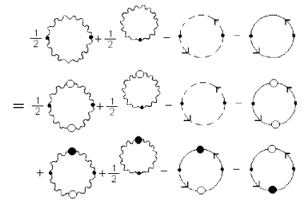
Figure 1: The diagrams contributing to the polarization tensor up to the second order in $g$ and all orders in the condensate parameters

The first four diagrams in this figure  represent the  usual second-order contribution to $\ \Pi_{\mu\nu}$ ,which is known to be transversal.  The condensate-dependent term  can also be represented as in Fig. 2.

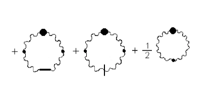
Figure 2: Condensate dependent contributions to the polarization tensor.

Note the absence of terms coming form the quark condensate. This is a consequence of the vanishing of these terms, which is directly due to the fact that a trace of an odd number of $\gamma$ matrices appears in their analytic expressions.     Further the last two diagrams in Fig. 2 were the ones evaluated in Ref. epjc in the Feynman gauge and whose result is transversal.  Finally, the analytic expression of the first diagram can be written in the form

$$T_{\mu\nu}=\frac{(1-\alpha)C_{q}}{(2\pi)^{D}i}(-g^{2})f^{a_{1}a_{2}a}f^{a_{1}a_{2}b}V_{\alpha\beta\mu}(0,p,-p)g^{\alpha\alpha^{\prime}}V_{\alpha^{\prime}\sigma\nu}(0,p,-p)\frac{p^{\beta}p^{\sigma}}{(p^{2})^{2}},$$

which, after employing the function defining the 3-gluon vertex muta

$$V_{\mu_{1}\mu_{2}\mu_{3}}(k_{1},k_{2},k_{3})=(k_{1}-k_{2})_{\mu_{3}}g_{\mu_{1}\mu_{2}}+(k_{2}-k_{3})_{\mu_{1}}g_{\mu_{3}\mu_{2}}+(k_{3}-k_{1})_{\mu_{2}}g_{\mu_{1}\mu_{3}},$$

leads to

$$T_{\mu\nu}^{ab}=\frac{(1-\alpha)C_{q}g^{2}}{(2\pi)^{D}i}f^{a_{1}a_{2}a}f^{a_{1}a_{2}b}\left(g_{\mu\nu}-\frac{p_{\mu}p_{\nu}}{p^{2}}\right),$$

showing the transversality of the polarization tensor up to second order in $g$ and all orders in the gluon and quark condensate parameters.    The  $\alpha$  independence of the effective action in the same approximation will be studied below.

V.2 $\alpha-$independence of the effective action in order $g^{2}$

Figure 3 shows the  terms of order 2 in the coupling constant (and any order in the other two parameters) of the effective action, evaluated at the zero value of the external fields. Expanding the gluon propagator as a sum of its Feynman gauge component plus the longitudinal and condensate parts; and the quark one as the usual Feynman propagator plus the quark$-$condensate part, the effective action can be expressed as shown in Fig. 3.

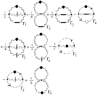
Figure 3: Diagrams representing the contributions to the effective action in the second order in $g$ and all order in the gluon and quark condensates

Observing this figure, it can be noted that the whole $\alpha$-dependent contribution is given by the first four diagrams. However, the first two of them vanish because the longitudinal propagator is contracted with the polarization tensor in the $g^{2\text{ }}$ approximation, which is transverse. Further,   the third term also vanishes thanks to the fact that the longitudinal propagator  is contracted with the particular self-energy part, which was shown, in the last subsection to be transverse by itself.  Finally, the  self-energy quark term in the fourth diagram identically vanishes, because of a trace of an odd number of  $\gamma$  matrices. This completes the proof of the gauge invariance of the effective action in second order in the coupling constant and any order of the condensate parameters.

In concluding this section it can be remarked that since massless QCD has no initial dimensional parameter, the removal of the dimensional regularization  in the diagrams of the theory can be done only after partial summations are performed. These summations, then, will input the new dimensional parameters associated to the condensates, implementing in this way the dimensional transmutation effect colewein . This and other issues are expected to be addressed in next works.

VI Summary

The gauge-invariance and regularization properties of the perturbative expansion for QCD considered in Refs. 1995 ; PRD ; epjc ; jhep was investigated. If follows that the singularities produced by the Dirac delta- function form of the new terms added to the gluon and quark propagators, can be properly eliminated by combining dimensional regularization liebbrandt with the infrared regularization procedure for the operator quantization of gauge theories Nakanishi . The dimensional extension allows to cancel the singular diagrams in which factors $\delta(0)$ appears due to the momentum conservation laws at vertices, when all lines arriving are associated to condensate $\delta$-like contributions. Further, the Nakanishi infrared procedure allows to get rid of the singularities in the form of a Feynman propagator evaluated at zero momentum.

Those factors appear when $n-1$ lines joined to a vertex of $n$ legs are of the condensate kind, and the remaining one is a Feynman propagator. In connection with the gauge-invariance properties, it is argued that the modified expansion should satisfy the same WTS identities as the usual PQCD. In addition, it follows that the formal functional integral representation of the generating functional of the Green functions only differs from the one associated to PQCD in the boundary conditions for the fields at $t=\pm\infty$. The formal functional integral results are checked in the second order in the coupling constant and any order in the condensate parameters. Firstly, the transversality of the gluon self-energy in the mentioned orders is shown. Afterwards, the contributions to the effective action evaluated at vanishing values of the mean fields, is shown to be gauge-parameter-independent. The work is expected to be extended in various directions. One of them is to implement the partial summations of the diagrams, the possibility of what was advanced in the text. This is needed in order to make the dimensional transmutation effective, thus, allowing to perform calculation depending on the new dimensional condensate parameters. Another activity to be considered will be to specify the renormalization procedure, which in the present problem involves three parameters. Finally, a task of direct physical interest will be to incorporate the knowledge about the invariance properties gained in the present work. It could bring a better understanding the results for the effective potential obtained in Ref. cabdann , in the Feynman gauge $\alpha=1$. The effective potential calculated in this work gave signals of a strong instability of massless QCD, under the generation of a quark condensate. But, it was precisely the possibility of this outcome, that was the main motivation for introducing the quark condensate in the initial free vacuum in epjc ; jhep . Therefore, the check of the re-appearance of the instability result within a gauge invariant calculation will give further support to the dynamical generation of quark masses and condensates within massless QCD.

Appendix A Kugo-Ojima quantization procedure for QCD

The main elements of the Kugo$-$Ojima operator quantization of the free massless QCD for an arbitrary gauge parameter $\alpha$ will be reviewed in this appendix. The formulae will be used in the construction of the modified perturbative expansion done in Section 2.  The classical action for the interacting fields in the Kugo-Ojima analysis has the form

$$S = \int dx\left(\mathcal{L}_{g}+\mathcal{L}_{gh}+\mathcal{L}_{B}+\mathcal{L}_{q}\right),$$

$$\mathcal{L}_{g} = -\frac{1}{4}F_{\mu\nu}^{a}(x)F^{a\mu\nu}(x),$$

$$\mathcal{L}_{gh} = -i\partial^{\mu}c^{a}(x)D_{\mu}^{ab}(x)c^{b}(x),$$

$$\mathcal{L}_{q} = \overline{\psi}^{r}(x)(i\gamma^{\mu}D_{\mu}^{rs}(x)-m\delta^{rs})\psi^{s}(x),$$

$$F_{\mu\nu}^{a}(x) = \partial_{\mu}A_{\nu}^{a}-\partial_{\nu}A_{\mu}^{a}+gf^{abc}A_{\mu}^{b}A_{\nu}^{c},$$

$$D_{\mu}^{ab}(x) = \delta^{ab}\partial_{\mu}-gf^{abc}A_{\mu}^{c},$$

$$D_{\mu}^{rs}(x) = \delta^{rs}\partial_{\mu}-gT_{c}^{rs}A_{\mu}^{c},$$

$$[T_{a},T_{b}] = if^{abc}T_{c}.$$

The equations of motion for the gluon, quarks, ghosts and auxiliary $B$ fields for a gauge parameter $\alpha$, in the Kugo and Ojima quantization scheme for free massless QCD take the form Kugo ; OjimaTex

$${\ \partial^{2}}A_{\mu}^{a}\left(x\right)-\left(1-\alpha\right)\partial_{\mu}\text{ }B^{a}\left(x\right) =0,$$

$$\partial^{\mu}A_{\mu}^{a}\left(x\right)+\alpha B^{a}\left(x\right) =0,$$

$${\ \partial^{2}}B^{a}\left(x\right)={\ \partial^{2}}\text{ }c^{a}\left(x\right)={\ \partial^{2}}\text{ }\overline{c}^{a}\left(x\right) =(i\text{ }\gamma^{\mu}\partial_{\mu}\,-m)\psi(x)=0,$$ (52)

where, for the moment, quark fields are also considered as having an auxiliary small mass $m$. The notation for the Lorentz indices and field quantities will follow the ones used in Ref. muta .  In the case of a general value of $\alpha$, the solution for the gluon field operator is the only one that differs from its counterpart in the Feynman gauge $\alpha=1,$ which was considered in Ref. PRD .  As derived in Kugo ; OjimaTex , the non-vanishing commutation relations among the fields have the forms

$$\left[A_{\mu}^{a}\left(x\right),A_{\nu}^{b}\left(y\right)\right] =-\delta^{ab}\left(g_{\mu\nu}D\left(x-y|0\right)-\left(1-\alpha\right)\partial_{\mu}\partial_{\nu}E\left(x-y\right)\right),$$

$$\left[A_{\mu}^{a}\left(x\right),B^{b}\left(y\right)\right] =\delta^{ab}\left(-\partial_{\mu}D\left(x-y|0\right)\right),$$

$$\left\{c^{a}\left(x\right),\overline{c}^{b}\left(y\right)\right\} =i\text{ }\delta^{ab}D\left(x-y\text{ }|\,0\right),\text{ \ \ }\left\{\psi\left(x\right),\overline{\psi}\left(y\right)\right\}=\delta^{rs}\text{ }(i\gamma^{\mu}\partial_{\mu}+m)D\left(x-y\text{ }|\,0\right),$$

$$D\left(z\text{ }|\,m\right) =\frac{1}{(2\pi)^{3}}\int dk\text{ }s(k_{0})\text{ }\delta(k^{2}-m^{2})\exp(-ik.z),\text{ \ }E\left(z\right)=\frac{1}{2}\frac{1}{\nabla_{z}^{2}}\left(z_{0}\frac{\partial}{\partial z_{0}}-1\right)\lim_{m\rightarrow 0}D\left(z\text{ }|\,m\right),$$

$$s(x) =\theta(x)-\theta(-x).$$

The invariant function $E$ appear in the commutation relations for the gluon field  when the  gauge parameter differs from the Feynman gauge value $\alpha=1$, since not all the gluon fields satisfy the D’Alembert equation. More generally, functions $E_{(\cdot)}$ are associated to each of the invariant  functions $D,D_{+},D_{-}$ and $D_{F}$ according to

$$E_{(\cdot)}\left(z\right)=-\lim_{m\rightarrow 0}\frac{\partial}{\partial m^{2}}D_{(\cdot)}\left(z\text{ }|\,m\right)\text{ }=\frac{1}{2}\frac{1}{\nabla_{z}^{2}}\left(z_{0}\frac{\partial}{\partial z_{0}}-1\right)\lim_{m\rightarrow 0}D_{(\cdot)}\left(z\text{ }|\,m\right).$$ (53)

where $(\cdot)$ means any  of the subindexes of the functions  $D,D_{+},D_{-}$ or $D_{F}.$

The gluon and Nakanishi $B$-field operators solving the above equations of motion are given as Kugo ; OjimaTex

$$A_{\mu}^{a}\left(x\right) =\sum\limits_{\vec{k}}\left(\sum\limits_{\sigma=1,2}A_{\vec{k},\sigma}^{a}f_{k,\mu}^{\text{ \ }\sigma}\left(x\right)+A_{\vec{k}}^{L,a}f_{k,L,\mu}\left(x\right)+B_{\vec{k}}^{a}\left[f_{k,S,\mu}\left(x\right)+(1-\alpha)\partial_{\mu}D_{(x)}^{(1/2)}g_{k}(x)\right]\right)+\text{h.c.},$$ (54)

$$B^{a}(x) =\sum\limits_{\vec{k}}B_{\vec{k}}^{a}g_{k}(x)+\text{h.c.},\text{ \ \ }c^{a}\left(x\right)=\sum\limits_{\vec{k}}c_{\vec{k}}^{a}\text{ }g_{k}(x)+h.c.,\text{ \ \ \ \ \ }\overline{c}^{a}\left(x\right)=\sum\limits_{\vec{k}}\overline{c}_{\vec{k}}^{a}\text{ }g_{k}(x)+\text{h.c.},$$ (55)

$$\psi(x) =\sum\limits_{\vec{k},s}\frac{1}{\sqrt{2V}}(a_{\vec{k}}^{s}\text{ }u_{\vec{k}}^{s}\text{ }\exp(-i\text{ }kx)+b_{\vec{k}}^{s+}v_{\vec{k}}^{s}\text{ }\exp(+i\text{ }kx)),$$ (56)

$$\overline{\psi}(x) =\sum\limits_{\vec{k},s}\frac{1}{\sqrt{2V}}(b_{\vec{k}}^{s}\overline{v}_{\vec{k}}^{s}\text{ }\exp(-i\text{ }kx)+a_{\vec{k}}^{s+}\text{ }\overline{u}_{\vec{k}}^{s}\text{ }\exp(+i\text{ }kx)),\text{\ \ \ \ \ \ }$$ (57)

where h.c. means the Hermitian conjugate of the previous term. The wave packets $g$ and $f$, the polarization vectors $\ \epsilon_{\mu}^{\sigma}\left(k\right)$, $\epsilon_{L,\text{\thinspace}\mu}\left(k\right)$, $\epsilon_{S,\,\mu}\left(k\right),$ the dirac spinor $u$ and $\ v$, and the integro-differential operator  $D_{(x)}^{(1/2)}$appearing in (54) are defined as Kugo ; OjimaTex :

$$g_{k}\left(x\right) =\frac{1}{\sqrt{2V\text{ }k_{0}}}\exp\left(-i\,kx\right),\quad\text{\ \ \ \ \ \ }f_{k,\mu}^{\sigma}\left(x\right)=\frac{1}{\sqrt{2V\text{ }k_{0}}}\epsilon_{\mu}^{\sigma}\left(k\right)\exp\left(-ikx\right)\text{ \ \ },$$

$$kx =k_{0}x_{0}-\vec{k}.\vec{x},\ \ k_{0}=\left|\vec{k}\right|,$$ (58)

$$\vec{k}\cdot\vec{\epsilon^{\sigma}}\left(k\right) =0,\ \epsilon_{0}^{\sigma}\left(k\right)=0,\ \vec{\epsilon^{\sigma}}\left(k\right)\cdot\vec{\epsilon^{\tau}}\left(k\right)=\delta^{\sigma\tau},\text{ \ \ \ for \ }\sigma,\tau=1,2,$$ (59)

$$\epsilon_{L,\mu}\left(k\right) =-i\,k_{\mu}=-i\left(|\vec{k}|,-\vec{k}\right),\ \ \ \ \epsilon_{S,\mu}\left(k\right)=-i\frac{\overline{k}_{\mu}}{2\,|\vec{k}|^{2}}=\frac{-i\left(|\vec{k}|,\text{ }\vec{k}\right)}{2\,|\vec{k}|^{2}},$$ (60)

$$D_{(x)}^{(1/2)} \equiv\frac{1}{2}(\nabla^{2})^{-1}(x_{0}\partial_{0}-1/2),$$ (61)

$$\,u_{\overrightarrow{k}}^{s} \equiv\,u^{s}(k)=\sqrt{m+k_{0}}\begin{pmatrix}u^{s}(0)\\ \frac{\overrightarrow{\sigma}\cdot\overrightarrow{k}}{m+k_{0}}u^{s}(0)\end{pmatrix},\,\text{\ \ \ \ \ \ \ \ }v_{\overrightarrow{k}}^{s}\equiv\,v^{s}(k)=\sqrt{m+k_{0}}\begin{pmatrix}\frac{\overrightarrow{\sigma}\cdot\overrightarrow{k}}{m+k_{0}}v^{s}(0)\\ v^{s}(0)\end{pmatrix}^{T}$$ (62)

The operator $D_{(x)}^{(1/2)}$ works as an “inverse” of the D’Alembertian for simple pole functions Nakanishi , that is

$$\partial^{2}D_{(x)}^{(1/2)}f\left(x\right)=f\left(x\right)\text{ \quad if \ \ }\partial^{2}\,f\left(x\right)=0.$$

A large cubic box of volume $V=L^{3}$ in a particular Lorentz reference frame is assumed for the imposition of periodic boundary conditions on the fields. Accordingly, the spatial momenta in the above sums take the values $\ \vec{k}=\frac{2\pi}{L}(n_{1},n_{2},n_{3}),$ for arbitrary integers $n_{1},n_{2}$   and $n_{3}.$ The four-vectors for all the particles but the quarks are null ones, $k=(|\,\vec{k}\,|,\vec{k}),$ and for the quarks $k=(\sqrt{|\vec{k}\,|^{2}+m^{2}},\,\vec{k}).$ The table below shows the commutation relations between the creation and annihilation operators for the various fields

$$\begin{Bmatrix}&A_{\vec{k}^{\prime},\lambda^{\prime}}^{a^{\prime}+}&A_{\vec{k}^{\prime}}^{L,a^{\prime}+}&B_{\vec{k}^{\prime}}^{a^{\prime}+}&c_{\vec{k}^{\prime}}^{a^{\prime}+}&\overline{c}_{\vec{k}^{\prime}}^{a+}&a_{\vec{k}^{\prime}}^{r^{\prime}+}&b_{\vec{k}^{\prime}}^{r^{\prime}+}\\ A_{\vec{k},\lambda}^{a}\ \ &\delta^{aa^{\prime}}\delta_{\vec{k}\vec{k}^{\prime}}\delta_{\lambda\lambda^{\prime}}&0&0&0&0&0&0\\ A_{\vec{k}}^{L,a}&0&0&-\delta^{aa^{\prime}}\delta_{\vec{k}\vec{k}^{\prime}}&0&0&0&0\\ B_{\vec{k}}^{a}&0&-\delta^{aa^{\prime}}\delta_{\vec{k}\vec{k}^{\prime}}&0&0&0&0&0\\ c_{\vec{k}}^{a}&0&0&0&0&i\,\delta^{aa^{\prime}}\delta_{\vec{k}\vec{k}^{\prime}}&0&0\\ \overline{c}_{\vec{k}}^{a}&0&0&0&-i\,\delta^{aa^{\prime}}\delta_{\vec{k}\vec{k}^{\prime}}&0&0&0\\ a_{\vec{k}}^{r}&0&0&0&0&0&\delta^{rr^{\prime}}\delta_{\vec{k}\vec{k}^{\prime}}&0\\ b_{\vec{k}}^{r}&0&0&0&0&0&0&\delta^{rr^{\prime}}\delta_{\vec{k}\vec{k}^{\prime}}\end{Bmatrix}.$$ (63)

Appendix B Longitudinal and Scalar Modes contribution

The contribution of longitudinal and scalar modes is determined by the expression

$$\langle 0 \mid \exp\left[C_{3}^{*}\left(\alpha,P\right)B_{\vec{p}_{i}}^{a}A_{\vec{p}_{i}}^{L,a}+D^{*}\left(\alpha,P\right)B_{\vec{p}_{i}}^{a}B_{\vec{p}_{i}}^{a}\right]\times$$ (64)

$$\times\exp\left\{i\int dxJ^{\mu,a}\left(x\right)\left(A_{\vec{p}_{i}}^{L,a+}f_{p_{i},L,\mu}^{*}\left(x\right)+B_{\vec{p}_{i}}^{a+}\left[f_{p_{i},S,\mu}^{*}\left(x\right)+(1-\alpha)\left(A^{*}\left(p_{0},x_{0}\right)f_{p_{i},L,\mu}^{*}\left(x\right)+B_{\mu}^{*}\left(p_{i},x\right)\right)\right]\right)\right\}$$

$$\times\exp\left\{i\int dxJ^{\mu,a}\left(x\right)\left(A_{\vec{p}_{i}}^{L,a}f_{p_{i},L,\mu}\left(x\right)+B_{\vec{p}_{i}}^{a}\left[f_{p_{i},S,\mu}\left(x\right)+(1-\alpha)\left(A\left(p_{0},x_{0}\right)f_{p_{i},L,\mu}\left(x\right)+B_{\mu}\left(p_{i},x\right)\right)\right]\right)\right\}$$

$$\times\exp\left[C_{3}\left(\alpha,P\right)B_{\vec{p}_{i}}^{a+}A_{\vec{p}_{i}}^{L,a+}+D\left(\alpha,P\right)B_{\vec{p}_{i}}^{a+}B_{\vec{p}_{i}}^{a+}\right]\mid 0\rangle.$$

As in Refs. PRD ; tesis , we first calculate

$$\exp\left\{i\int dxJ^{\mu,a}\left(x\right)\left(A_{\vec{p}_{i}}^{L,a}f_{p_{i},L,\mu}\left(x\right)+B_{\vec{p}_{i}}^{a}\left[f_{p_{i},S,\mu}\left(x\right)+(1-\alpha)\left(A\left(p_{0},x_{0}\right)f_{p_{i},L,\mu}\left(x\right)+B_{\mu}\left(p_{i},x\right)\right)\right]\right)\right\}$$ (65)

$$\times\exp\left[C_{3}\left(\alpha,P\right)B_{\vec{p}_{i}}^{a+}A_{\vec{p}_{i}}^{L,a+}+D\left(\alpha,P\right)B_{\vec{p}_{i}}^{a+}B_{\vec{p}_{i}}^{a+}\right]\mid 0\rangle,$$

$$= \exp\left\{C_{3}\left(\alpha,P\right)\left(B_{\vec{p}_{i}}^{a+}-i\int dxJ^{\mu,a}\left(x\right)f_{p_{i},L,\mu}\left(x\right)\right)\right.\times$$

$$\qquad\quad\times\left(A_{\vec{p}_{i}}^{L,a+}-i\int dxJ^{\mu,a}\left(x\right)\left[f_{p_{i},S,\mu}\left(x\right)+(1-\alpha)\left(A\left(p_{0},x_{0}\right)f_{p_{i},L,\mu}\left(x\right)+B_{\mu}\left(p_{i},x\right)\right)\right]\right)$$

$$\quad\ \ \left.+D\left(\alpha,V\right)\left(B_{\vec{p}_{i}}^{a+}-i\int dxJ^{\mu,a}\left(x\right)f_{p_{i},L,\mu}\left(x\right)\right)\left(B_{\vec{p}_{i}}^{a+}-i\int d3xJ^{\mu,a}\left(x\right)f_{p_{i},L,\mu}\left(x\right)\right)\right\}\mid 0\rangle.$$

A similar expression is obtained acting to the left in Eq. (64). Substituting the above results in (64), and introducing the following notation,

$$C^{*} \equiv C_{3}^{*}\left(\alpha,P\right),\ C\equiv C_{3}\left(\alpha,P\right),\quad D^{*}\equiv D^{*}\left(\alpha,P\right),\ D\equiv D\left(\alpha,P\right),$$

$$\hat{A}^{+} \equiv A_{\vec{p}_{i}}^{L,a+},\ \hat{A}\equiv A_{\vec{p}_{i}}^{L,a},\quad\hat{B}^{+}\equiv B_{\vec{p}_{i}}^{a+},\ \hat{B}\equiv B_{\vec{p}_{i}}^{a},$$

$$a_{1} \equiv -i\int dxJ^{\mu,a}\left(x\right)\left[f_{p_{i},S,\mu}^{*}\left(x\right)+(1-\alpha)\left(A^{*}\left(p_{0},x_{0}\right)f_{p_{i},L,\mu}^{*}\left(x\right)+B_{\mu}^{*}\left(p_{i},x\right)\right)\right],$$

$$a_{2} \equiv -i\int dxJ^{\mu,a}\left(x\right)\left[f_{p_{i},S,\mu}\left(x\right)+(1-\alpha)\left(A\left(p_{0},x_{0}\right)f_{p_{i},L,\mu}\left(x\right)+B_{\mu}\left(p_{i},x\right)\right)\right],$$

$$b_{1} \equiv -i\int dxJ^{\mu,a}\left(x\right)f_{p_{i},L,\mu}^{*}\left(x\right),$$

$$b_{2} \equiv -i\int dxJ^{\mu,a}\left(x\right)f_{p_{i},L,\mu}\left(x\right),$$ (66)

one obtains

$$\langle 0\mid\exp\left\{C^{*}\left(\hat{A}+a_{1}\right)\left(\hat{B}+b_{1}\right)+D^{*}\left(\hat{B}+b_{1}\right)\left(\hat{B}+b_{1}\right)\right\}$$

$$\times\exp\left\{C\left(\hat{B}^{+}+b_{2}\right)\left(\hat{A}^{+}+a_{2}\right)+D\left(\hat{B}^{+}+b_{2}\right)\left(\hat{B}^{+}+b_{2}\right)\right\}\mid 0\rangle.$$ (67)

Following exactly the same procedure previously described in Refs. PRD ; tesis , a recurrence relation is obtained for Eq. (67).

$$\exp\left\{C^{*}a_{1}b_{1}+D^{*}b_{1}^{2}+\left[C\left(C^{*}a_{1}-a_{2}\right)+2CD^{*}b_{1}\right]\left(C^{*}b_{1}-b_{2}\right)\sum\limits_{m=0}^{n}\left[\left|C\right|^{2\left(2m\right)}+\left|C\right|^{2\left(2m+1\right)}\right]+\right.$$

$$\quad+\left(C^{*}b_{1}-b_{2}\right)^{2}\left(D\sum_{m=0}^{n}\left[\left(2m+1\right)\left|C\right|^{2\left(2m\right)}+2\left(m+1\right)\left|C\right|^{2\left(2m+1\right)}\right]+\right.$$

$$\quad\quad\left.\left.+C^{2}D^{*}\sum_{m=0}^{n}\left[2m\left|C\right|^{2\left(2m-1\right)}+\left(2m+1\right)\left|C\right|^{2\left(2m\right)}\right]\right)\right\}\langle 0\mid\exp\left\{C^{*}\hat{A}\hat{B}+D^{*}\hat{B}\hat{B}\right\}\times$$

$$\times\exp\left\{C^{*n+1}C^{n+1}\left(C^{*}b_{1}-b_{2}\right)\hat{A}+\left[C^{*n+1}C^{n+1}\left(C^{*}a_{1}-a_{2}\right)+2C^{*n+1}C^{n+1}D^{*}b_{1}+\right.\right.$$

$$\qquad+\left.\left.2C^{*n}C^{n}\left(n+1\right)\left(C^{*}D+CD^{*}\right)\left(C^{*}b_{1}-b_{2}\right)\right]\hat{B}\right\}\exp\left\{C\hat{B}^{+}\hat{A}^{+}+D\hat{B}^{+}\hat{B}^{+}\right\}\mid 0\rangle.$$ (68)

We then assume that $|C|<1$ so that in the limit $n\rightarrow\infty$

$$\lim_{n\rightarrow\infty}\left|C\right|^{2n}=\lim_{n\rightarrow\infty}n\left|C\right|^{2n}=0,$$

$$\lim_{n\rightarrow\infty}\sum\limits_{m=0}^{n}\left[\left|C\right|^{2\left(2m\right)}+\left|C\right|^{2\left(2m+1\right)}\right]=\frac{1}{\left(1-\left|C\right|^{2}\right)},$$

$$\lim_{n\rightarrow\infty}\sum_{m=0}^{n}\left[\left(2m+1\right)\left|C\right|^{2\left(2m\right)}+2\left(m+1\right)\left|C\right|^{2\left(2m+1\right)}\right]=\frac{1}{\left(1-\left|C\right|^{2}\right)^{2}},$$ (69)

which allows to rewrite Eq. (68) as

$$\exp\left\{C^{*}a_{1}b_{1}+D^{*}b_{1}^{2}+\left[C\left(C^{*}a_{1}-a_{2}\right)+2CD^{*}b_{1}\right]\frac{\left(C^{*}b_{1}-b_{2}\right)}{\left(1-\left|C\right|^{2}\right)}+\left(C^{*}b_{1}-b_{2}\right)^{2}\frac{\left(D+C^{2}D^{*}\right)}{\left(1-\left|C\right|^{2}\right)^{2}}\right\}$$

$$\langle 0\mid\exp\left\{C^{*}\hat{A}\hat{B}+D^{*}\hat{B}\hat{B}\right\}\exp\left\{C\hat{B}^{+}\hat{A}^{+}+D\hat{B}^{+}\hat{B}^{+}\right\}\mid 0\rangle.$$ (70)

Replacing the compact notation (66) in (70), and expanding all functions of $\vec{p}_{i}$ in the vicinity of $\vec{p}_{i}=0$ (keeping in mind that the sources are located in a space finite region), it’s sufficient to consider only the first term in all expansions. After that Eq. (70) takes the form (25).

References

• (1) T. Schäfer and E. V. Shuryak, Rev. Mod. Phys. 70, 323 (1998).
• (2) A. Cabo, S. Peñaranda, and R. Martinez, Mod. Phys. Lett. A10, 2413 (1995).
• (3) M. Rigol and A. Cabo, Phys. Rev. D62, 074018 (2000); hep-th/9909057.
• (4) A. Cabo and M. Rigol, Eur. Phys. J. C23, 289 (2002); hep-ph/0008003.
• (5) M. Rigol, About an Alternative Vacuum State for Perturbative QCD, Graduate Dissertation Thesis, Instituto Superior de Ciencias y Tecnología Nucleares, La Habana, Cuba, 1999.
• (6) A. Cabo, JHEP 04, 044 (2003), hep-ph/0209215(2002).
• (7) G. K. Savvidy, Phys. Lett. B71, 133 (1977).
• (8) I. A. Batalin, S. G. Matinyan, and G. K. Savvidy, Sov. J. Nucl. Phys. 26, 214 (1977).
• (9) A. Cabo, O. K. Kalashnikov and A.E. Shabad, Nucl. Phys. B185, 473 (1981).
• (10) W. Dittrich and M. Reuter, Phys. Lett. B128, 321 (1983).
• (11) P. Hoyer, HIP-2002-44-TH, Sep 2002. 3pp.; Talk given at 31st International Conference on High Energy Physics, ICHEP 367-369, Amsterdam; hep-ph/0209318 (2002).
• (12) M. A. Shifman, A. I. Vainshtein, and V. I. Zakharov, Nucl. Phys. B147, 385 (1979); B147, 448 (1979); B147, 519 (1979).
• (13) R. Fukuda, Phys. Rev. D21, 485 (1980).
• (14) K. G. Chetyrkin, S. Narison, and V. I. Zakharov, Nucl. Phys. B550, 353 (1999).
• (15) S. J. Huber, M. Reuter, and M. G. Schmidt, Phys. Lett. B462, 158 (1999).
• (16) P. Hoyer, NORDITA - 96/63 P (1996), hep-ph/9610270 (1996); P. Hoyer, NORDITA - 97/44 P (1997), hep-ph/9709444 (1997).
• (17) H. J. Munczek and A. M. Nemirovsky, Phys. Rev. D55, 3455 (1983).
• (18) C. J. Burden, C. D. Roberts, and A. G. Williams, Phys. Lett. B 285, 347 (1992).
• (19) T. Kugo and I. Ojima, Prog. Theor. Phys. Suppl. 66, 1 (1979).
• (20) N. Nakanishi and I. Ojima, Covariant Operator Formalism of Gauge Theories and Quantum Gravity, Singapore, Word Scientific, 1990.
• (21) H. P. Pavel, D. Blaschke, V. N. Pervushin, and G. Röpke, Int. J. Mod. Phys. A 14, 205 (1999).
• (22) N. Nakanishi, Prog. Theor. Phys. 51, 952 (1974); N. Nakanishi, Prog. Theor. Phys. 52, 1929 (1974).
• (23) D. G. Boulware, Phys. Rev. D23, 389 (1981).
• (24) B. S. DeWitt, in Proceedings: Symposium on Quantum Gravity II, Eds. C. Isham, R. Penrose and D. Sciama, Clarendon Press, Oxford, 1981.
• (25) G. ‘t Hooft, in 12th Winter School of Theoretical Physics Functional and Probabilistic Methods in Quantum Field Theory, Karpacz, Poland, 17 Feb - 2 Mar 1975, Acta Universitatis Wratislaviensis No.368, Eds. J. Lopuszánski and B. Jancewicz, Vol. 1, 1976.
• (26) G. Leibbrandt, Rev. Mod. Phys. 47, 849 (1975).
• (27) T. Muta, Foundations of Quantum Chromodynamics, World Scientific Lectures Notes in Physics - Vol. 5, 1987.
• (28) S. Gasiorowicz, Elementary Particle Physics, New York, Jonh Wiley & Sons, 1966.
• (29) L. D. Faddeev and A. A. Slanov, Gauge Fields. Introduction to Quantum Theory, Benjamin Cummings Publishing, 1980.
• (30) B. Sakita, Quantum Theory of Many Variable Systems and Fields, World Scientific Lecture Notes in Physics, Vol. 1, 1985.
• (31) J. Zinn-Justin, in Trends in Elementary Particle Theory, Lecture Notes in Physics, Vol. 37, Springer Verlag, 1975.
• (32) S. Coleman and E. Weinberg, Phys. Rev. D7, 1888 (1973).
• (33) A. Cabo and D. Martinez-Pedrera, ICTP Preprint IC/2004/118 (2004), hep-ph/0501054(2005).