Signatures of the Color Glass Condensate
in $J/\Psi$ production off nuclear targets

Abstract

We consider the $J/\Psi$ production in proton (deuteron) – nucleus collisions at high energies. We argue that the production mechanism in this case is different from that in $pp$ collisions due to gluon saturation in the nucleus and formation of the Color Glass Condensate. At forward rapidities (in the proton fragmentation region), the production of $J/\Psi$ is increasingly suppressed both as a function of rapidity and centrality. On the other hand, at backward rapidities at RHIC (in the fragmentation region of the nucleus) the coherent effects lead to a modest enhancement of the production cross section, with the nuclear modification factor $R_{J/\Psi}$ increasing with centrality. We find that the $J/\Psi$ production cross section exhibits at forward rapidities the limiting fragmentation scaling established previously for soft processes; in the energy range studied experimentally, it manifests itself as an approximate “$x_{F}$ scaling”.

I Introduction

Understanding the ${J/\Psi}$ production mechanism is one of the challenges of QCD. On one hand the charm quark mass is quite large on the typical QCD scale of $\Lambda_{\mathrm{QCD}}$, which makes the use of perturbative QCD meaningful collcharm since the long distance dynamics is effectively decoupled Appelquist:tg . However the size of this system and the inverse of the binding energy are not small enough to suppress significant non-perturbative contributions. Indeed, perturbative QCD fails in describing the differential ${J/\Psi}$ production cross section and the polarization. Different mechanisms were suggested to explain the existing experimental data. Unfortunately all of them so far have encountered problems in describing at least some of the observables (for a recent review, see Brambilla:2004wf ). In the context of high energy nuclear physics, it is important to understand well the mechanism of ${J/\Psi}$ production also in nuclear processes since ${J/\Psi}$ suppression in heavy-ion collisions could serve as a signal of the Quark-Gluon Plasma formation Matsui:1986dk .

One of the long-standing puzzles is the lack of $x_{2}$ scaling of the nuclear modification factor ($x_{2}$ is the Bjorken variable corresponding to the nuclear target parton distribution) in $J/\psi$ production off nuclei. Even though this scaling is expected to hold in the parton model, the data from CERN Badier:1983dg and FNAL Leitch:1999ea fixed target experiments are in violent contradiction with this expectation. The absence of $x_{2}$ scaling has become even more dramatic at RHIC Adler:2005ph . Instead of the badly broken $x_{2}$ scaling, the data instead exhibit an unexpected approximate scaling in the Feynman $x_{F}$ variable.

It was realized long time ago Brodsky:1991dj that this lack of $x_{2}$ scaling, and thus the violation of QCD factorization, is caused by multi-parton (higher twist) interactions in the nuclear target. Several specific mechanisms of this type were considered over the years Kopeliovich:1984bf ; Vogt:1991qd ; Gavin:1991qk ; Kharzeev:1993qd ; Clavelli:1985kg ; Benesh:1994du ; Fujii:2003ff .

In this paper we would like to re-visit the problem of ${J/\Psi}$ production in proton – nucleus collisions at high energy basing on the novel Color Glass Condensate picture of the nuclear wave function at small $x$. In this approach, the strength of the color field inside the nucleus is proportional to the saturation scale $Q_{s}^{2}(x_{2})$ determined by the density of partons in the transverse plane. It is a growing function of the collision energy and the atomic number of the nucleus. Experimental data indicate that at RHIC kinematics $Q_{s}\gg\Lambda_{\mathrm{QCD}}$ which implies that the inter-nucleon interactions play a little role in pA interactions at high energies. Therefore, at high energies a nuclear color field can be described by only one universal (process independent) dimensional scale $Q_{s}(x_{2})$ GLR ; Mueller:wy ; Blaizot:nc ; MV . The production of heavy quarks in this framework has been previously considered in several papers KhT ; KTcc ; Gelis:2003vh ; Blaizot:2004wv ; Gelis:2004jp ; Fujii:2005vj .

In the previous publications KhT ; KTcc , we have argued that there are two different dynamical regimes of heavy quark production at high energies depending on the relation between the saturation scale and the quark’s mass $m$. When $Q_{s}\ll m$ the heavy quark production is incoherent, meaning that it is produced in a single sub-collision of a proton with a nucleon. This case can be treated within a conventional perturbative approach. In the opposite limit of $Q_{s}\gg m$ the heavy quark production is coherent since the whole nucleus takes part in the process. In this case the heavy quark production is sensitive to a strong color field (CGC) which violates the decoupling of the subprocess of heavy quark production from the dynamics of partons in the nuclear wave function LRSS ; KhT . The reason is that the decoupling theorems can be applied only when the heavy quark mass is much larger than the typical hadronic scale, which is of the order of $Q_{s}(x)$ at high energies.

The goal of this paper is to address the problem of ${J/\Psi}$ production at high energies. It is organized as follows. In section II we argue that at high energies the time of interaction of the projectile proton with the target nucleus at rest is much smaller than the time of heavy quark pair production and subsequent formation of a bound state. This will allow us to use the eikonal approximation and derive in section III the cross section for the ${J/\Psi}$ production in pA collisions at high energies. In section IV we study the derived expression in two different kinematical regions. We show that at $Q_{s}\ll M_{\psi}$ the ${J/\Psi}$ the cross section is an increasing function of centrality since the dominant contribution comes from the two-gluon exchange process. At $Q_{s}\gg M_{\psi}$ multiple re-scattering as well as quantum evolution lead to the suppression of ${J/\Psi}$ production both as a function of energy/rapidity and centrality. We also point out that the approximate $x_{F}$ scaling observed in SPS and FNAL data emerges naturally in our approach. However, it is seen to be a consequence of the slow dependence of the gluon distribution on energy, and so is broken at higher energies. However, as the energy increases (e.g. to the LHC energy range) the $x_{F}$ scaling is restored owing to the onset of gluon saturation in the incident proton. We compare our calculations with the available experimental data in Sec.  V and conclude in Sec. VI.

II Different production mechanisms of ${J/\Psi}$ on nucleus

II.1 Relevant time scales

Consider charmonium production in a pA collision. A $c\bar{c}$ pair is produced over the time $1/(2m_{c})$ in its center-of-mass frame. In the nucleus rest frame this time is Lorentz-dilated MuBr ; KZ

$$\tau_{P}\,\approx\,\frac{1}{(2\,m_{c})}\,\frac{E_{g}}{(2\,m_{c})}\,,$$ (1)

where $E_{g}$ is a parent gluon’s energy. This time scale should be compared to the typical interaction time $\tau_{\mathrm{int}}\sim R_{A}/c$. Eq. (1) shows that at very high energies the production time of $c\bar{c}$ pair can be much larger than the interaction time $\tau_{P}\,\gg\,\tau_{\mathrm{int}}$. This a general property of all hard processes at high energies: they develop over a long time $\tau_{P}$ Ioffe .

This formula can be rewritten in terms of the Bjorken variable associated with nucleus, $x_{2}$. Note, that the gluon takes fraction $x_{1}$ of the proton’s energy $E_{g}\,=\,x_{1}\,E_{p}$. Also, by four-momentum conservation, $(2\,m_{c})^{2}\,=\,x_{1}\,x_{2}\,s\,=\,2\,x_{1}\,x_{2}\,M_{N}\,E_{p}$, where $M_{N}$ is the nucleon mass and $E_{p}$ is the proton’s energy. Thus, it follows from (1) that

$$\tau_{P}\,\approx\,\frac{1}{2\,M_{N}\,x_{2}}\,.$$ (2)

At RHIC, in the center-of-mass frame $x_{2}\,=\,(m_{c}/\sqrt{s})\,e^{-y}\,=\,6.5\cdot 10^{-3}\,e^{-y}$, where we introduced rapidity $y$. Therefore,

$$\tau_{P}(\mathrm{RHIC})\,\approx\,15\,e^{y}\,\mathrm{fm}.$$ (3)

Equation (3) implies that at forward rapidities $y>1$ one can indeed assume that the proton interacts coherently with the whole nucleus (similar estimates for the fixed target energies can be found in Kharzeev:1995id ). In this case the transverse size of the $c\bar{c}$ pair is fixed during its propagation through the nucleus and we can apply the eikonal approximation for calculation of the scattering amplitude NZ ; AMdipole .

Finally, the ${J/\Psi}$ wave function is formed from the initial $c\bar{c}$ pair. This lasts $\sim\,2/(M_{\Psi^{\prime}}-M_{\Psi})$ in the ${J/\Psi}$ rest frame. In the nucleus rest frame the ${J/\Psi}$ formation time is MuBr ; KZ

$$\tau_{F}\,\approx\,\frac{2}{M_{\Psi^{\prime}}-M_{\psi}}\,\frac{E_{g}}{M_{\psi}}\,.$$ (4)

Since the ${J/\Psi}$ bounding energy is much less than its mass, the ${J/\Psi}$ production time is much shorter than its formation time: $\tau_{P}\,\ll\,\tau_{F}$. A more accurate evaluation of the formation time can be performed with the help of the spectral representation for the ${J/\Psi}$ propagator by using the experimental data on $e^{+}e^{-}$ annihilation into charm quarks Kharzeev:1999bh ; this leads to the ${J/\Psi}$ proper formation time of $0.45$ fm. Thus, at RHIC

$$\tau_{F}(\mathrm{RHIC})\,\approx\,41\,e^{y}\,\mathrm{fm};$$ (5)

the ${J/\Psi}$ wave function is therefore formed outside of the nucleus at rapidities $y\,{{}_{\displaystyle{>}}\atop\displaystyle{\sim}}\,-2$.

The relationships between the three relevant time scales $\tau_{\mathrm{int}}$, $\tau_{P}$ and $\tau_{F}$ depend on the collision energy $\sqrt{s}$ and the rapidity $y$. In the next subsection we classify all possible situations in the RHIC kinematical region ($\sqrt{s}\,=\,200$ GeV).

II.2 Coherent versus incoherent ${J/\Psi}$ production

II.2.1 Forward rapidities

At (pseudo)-rapidities $y\,{{}_{\displaystyle{>}}\atop\displaystyle{\sim}}\,1$ $\tau_{F}\,\gg\,\tau_{P}\,\gg\tau_{\mathrm{int}}$. This implies that the $c\bar{c}$ pair scatters coherently off all the nucleons along its trajectory in the nucleus, see Fig. 1. Therefore, the process of ${J/\Psi}$ formation proceeds through the following three stages in the nucleus rest frame. First, way before the collision with the nucleus, the fast proton develops a cloud of virtual partons which includes one $c\bar{c}$ pair (in the leading order in $\alpha_{s}$). In the light-cone perturbation theory this is described by the valence quark and the virtual gluon wave functions which are explicitly displayed in the next section, see III.2. Second, the coherence of the cloud is destroyed by interaction with nucleons in nucleus. Due to the large production time $\tau_{P}$ the scattering matrix can be diagonalized in the color dipole basis: the transverse size of the $c\bar{c}$ is fixed during the interaction. We calculate the $c\bar{c}A$ amplitude in section III.1. Third, ${J/\Psi}$ is formed far away from the nuclear remnants. No nuclear effects are expected at this stage.

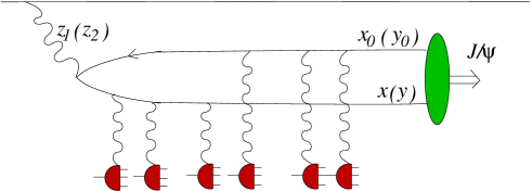
Figure 1: Production of ${J/\Psi}$ in pA collisions at high energy. At RHIC $\sqrt{s}=200$ GeV: $y{{}_{\displaystyle{>}}\atop\displaystyle{\sim}}2$.

II.2.2 Central rapidities

At rapidities $-1\,{{}_{\displaystyle{<}}\atop\displaystyle{\sim}}\,y\,{{}_{\displaystyle{<}}\atop\displaystyle{\sim}}\,0$ the production time becomes smaller than the nuclear size which implies that the $c\bar{c}$ pair scatters coherently off a few nucleons. This leads to the enhancement of ${J/\Psi}$ production since in that case the main contribution to the scattering amplitude arises from the diagram shown in Fig. 2(a) which is enhanced by an additional power of $A^{1/3}$ with respect to the diagram Fig. 2(b) which describes ${J/\Psi}$ production in pp collisions.

The diagram Fig. 2(a), where the ${J/\Psi}$ is produced by double gluon exchange is parametrically enhanced compared to the diagram shown in Fig. 2(b) where the ${J/\Psi}$ is produced by one gluon exchange. Indeed, let us for a moment concentrate on ${J/\Psi}$ production in a quasi-classical approximation where the coupling is small $\alpha_{s}(Q_{s}^{2})\ll 1$ and together with atomic number $A\gg 1$ it forms a resummation parameter $\alpha_{s}^{2}A^{1/3}\sim 1$ YuK . The diagram (b) in Fig. 2 is of the order $\alpha_{s}^{5}A^{1/3}\sim\alpha_{s}^{3}$ while the diagram (a) is of the order of $\alpha_{s}^{6}A^{2/3}\sim\alpha_{s}^{2}$. Therefore, the diagram (a) is enhanced provided that the nucleus is sufficiently large.

This conclusion remains valid beyond the quasi-classical approximation. The gluons emitted in the course of quantum evolution get resummed into gluon distribution functions, which therefore grow fast as $x$ decreases. The resummation parameter $\alpha_{s}\,xG(x,Q^{2})\,A^{1/3}$ becomes large even for the proton GLR . At small enough $x$ the diagram (a) dominates the ${J/\Psi}$ production even for the scattering off light nuclei $A\sim 1$. The general effect of the enhancement of double-gluon exchange diagrams in hard processes on heavy nuclei has been already pointed out by in Brodsky:1991dj ; HKZ .

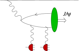
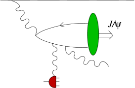
(a)		(b)

Figure 2: Two mechanisms of ${J/\Psi}$ production: (a) by two-gluon exchange; (b) by one-gluon exchange and one-gluon emission.

Although the dipole model qualitatively describes the effect of the enhancement of ${J/\Psi}$ production at $-1\,{{}_{\displaystyle{<}}\atop\displaystyle{\sim}}\,y\,{{}_{\displaystyle{<}}\atop\displaystyle{\sim}}\,0$ it cannot be applied at $y\,{{}_{\displaystyle{<}}\atop\displaystyle{\sim}}\,0$ due to the effect of finite production time. In other words to get a reasonable description of the process one has to include the absorption corrections of the color dipole $c\bar{c}$ in the nuclear medium (note that $\tau_{F}$ is still much larger than $R_{A}$). In the present publication we are going to analyze only $y>0$ region at RHIC. However when comparing to the experimental data from CERN and FNAL we will have to correct the results by the absorption factors, see Sec. V.2.

To quantify the effect of the finite production time and to specify the region of applicability of eikonal approximation, we can consider the longitudinal nuclear form factor $F_{A}^{2}(q_{z})$, which takes into account the quantum interference in the longitudinal direction at a finite longitudinal momentum transfer Gribov:1969zy (this formfactor is assumed to equal unity in the dipole model). It is defined as

$$F_{A}^{2}(q_{z})\,=\,A^{-1}\,\int d^{2}b\,\left|\,\int_{-\infty}^{\infty}dz\,\rho(b,z)\,e^{i\,q_{z}\,z}\,\right|^{2}\,,$$ (6)

where $q_{z}$ is the longitudinal momentum transfer and $\rho(b,z)$ is the density of nucleons in a nucleus. The typical value of the longitudinal coordinate in (6) is $z\sim R_{A}$. Therefore, the integral over $z$ vanishes due to rapid oscillations of the exponential factor unless $q_{z}\,<\,1/R_{A}$. On the other hand $q_{z}\,\sim\,1/\tau_{P}$. Thus, $F_{A}(q_{z})$ is sizable (it is normalized to unity) when $\tau_{P}\,>\,R_{A}$ and is small otherwise.

Assuming for simplicity a Gaussian parameterization of the nuclear density we obtain $F_{A}^{2}(q_{z})\,=\,e^{-R_{A}^{2}\,q_{z}^{2}/3}$ HKZ . In the Fig. 3 we plot the longitudinal form factor for different energies.

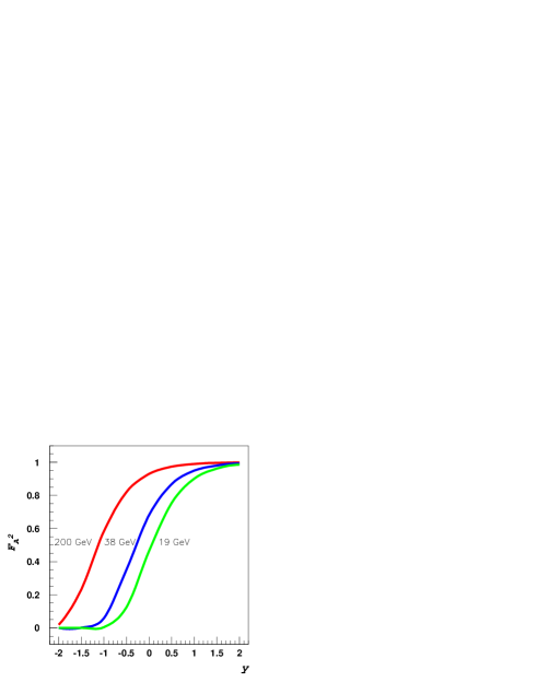
Figure 3: The longitudinal form factor $F_{A}^{2}$ as a function of rapidity $y$ for RHIC, Tevatron and SPS energies.

We learn from Fig. 3 that the corrections to the dipole model due to a finite $\tau_{P}$ are of the order of 10% at $y=0$ at RHIC ($\sqrt{s}=200$ GeV), but already at $y=-1$ they are as large as 50%. Therefore, the dipole model should provide an accurate result for $y\,{{}_{\displaystyle{>}}\atop\displaystyle{\sim}}\,0$ which correspond to $x_{F}\,{{}_{\displaystyle{>}}\atop\displaystyle{\sim}}\,0$. At Fermilab fixed target experiments ($\sqrt{s}=38$ GeV) the dipole model is applicable (corrections ${{}_{\displaystyle{<}}\atop\displaystyle{\sim}}$ 10%) at rapidities larger than $\sim\ln(200/38)=1.7$ which correspond to $x_{F}\,\simeq\,0.4$. At SPS ($\sqrt{s}\,=\,19$ GeV) the dipole model has to be corrected even in the most forward region.

II.2.3 Backward rapidities

At rapidities $y\,{{}_{\displaystyle{<}}\atop\displaystyle{\sim}}\,-2$ the coherence is completely lost and the process of ${J/\Psi}$ production in pA collisions becomes similar to the one in pp collisions. All of the dependence on $A$ arises then from the propagation of the produced $c\bar{c}$ pair and ${J/\Psi}$ through the nuclear matter.

III Cross section for ${J/\Psi}$ production at forward rapidities.

III.1 Propagation of the $c\bar{c}$ pair through the nucleus

The first step in calculation of the ${J/\Psi}$ production cross section, see Fig. 1 , is the calculation of the scattering amplitude of $q_{v}c\bar{c}$ state off the nucleus with the projection on the color neutral state after the $c\bar{c}$ passes the nucleus. In our analysis we will assume, for the sake of simplicity, that the valence quark is a spectator.

It is straightforward, although laborious, to calculate all possible gluon attachments to quark and antiquark in Fig. 1. In the large $N_{c}$ approximation the $c\bar{c}$ amplitude for a single scattering (Fig. 2) projected on the color singlet state reads

$$\mathcal{M}_{1}(\underline{x},\underline{x}_{0},\underline{y},\underline{y}_{0})=\frac{1}{4}\bigg{(}\frac{Q_{s}^{2}}{4}\bigg{)}^{2}\,\bigg{[}(\underline{x}-\underline{y})^{2}\,+\,(\underline{x}_{0}-\underline{y}_{0})^{2}\bigg{]}^{2}\,.$$ (7)

The saturation scale $Q_{s}^{2}$ in (10) is given by AlMu

$$Q_{s}^{2}(\underline{x})=\frac{4\pi^{2}\alpha_{s}N_{c}}{N_{c}^{2}-1}\,\rho\,T(\underline{b})\,xG(x,1/\underline{x}^{2}),$$ (8)

where the gluon distribution function in the nucleon reads

$$xG(x,1/\underline{x}^{2})=\frac{\alpha_{s}\,C_{F}}{\pi}\,\ln\frac{1}{\underline{x}^{2}\mu^{2}},$$ (9)

where $\mu$ is some infrared cutoff. For a spherical sharp-edge nucleus $T(\underline{b})=2\sqrt{R^{2}-\underline{b}^{2}}$.

Assuming that the scatterings off the individual nucleons are independent, one can generalize (7) to include multiple rescatterings (see Fig. 1) in a straightforward way. The $q\bar{q}A$ amplitude then takes the form

$$\mathcal{M}(\underline{x},\underline{x}_{0},\underline{y},\underline{y}_{0})=1\,-\,\exp\bigg{\{}-\frac{1}{4}\bigg{(}\frac{Q_{s}^{2}}{4}\bigg{)}^{2}\,\bigg{[}(\underline{x}-\underline{y})^{2}\,+\,(\underline{x}_{0}-\underline{y}_{0})^{2}\bigg{]}^{2}\bigg{\}}$$ (10)

We checked that the color factor exponentiates using the FeynCalc package feyncalc .

III.2 Wave functions

In view of the arguments given in the previous section, at forward rapidities the processes of formation of the proton wave function, the subsequent rescatterings of the proton’s partons inside the target nucleus and the formation of the bound $c\bar{c}$ state are well separated in time in the nucleus rest frame. Hence, to proceed we need to know the light-cone wave functions of the valence quark, the virtual gluon and the ${J/\Psi}$. In the $A_{+}=0$ light cone gauge the valence quark’s wave function in the configuration space reads AMdipole

$$\Psi_{q_{v}\rightarrow q_{v}g}(\underline{z})=\int\,\frac{d^{2}q}{(2\pi)^{2}}\,e^{-i\,\underline{q}\cdot\underline{z}}\,\Psi_{q_{v}\rightarrow q_{v}g}(\underline{q})=g\,T^{a}\,\frac{1}{2\pi i}\,\frac{\underline{\epsilon}^{\lambda}\cdot\underline{z}}{\underline{z}^{2}},$$ (11)

Averaging the square of Eq. (11) over the quantum numbers of the initial quark and summing over the quantum numbers of the final quark and gluon we obtain the familiar gluon radiation kernel of a dipole model

$$\Phi_{q_{v}\rightarrow q_{v}g}(\underline{z}_{1},\underline{z}_{2})=\frac{1}{2N_{c}}\,\sum_{a,\lambda}\Psi_{q_{v}\rightarrow q_{v}g}(\underline{z}_{1})\Psi^{*}_{q_{v}\rightarrow q_{v}g}(\underline{z}_{2})=\frac{\alpha_{s}C_{F}}{2\pi}\,\frac{\underline{z}_{1}\cdot\underline{z}_{2}}{\underline{z}_{1}^{2}\,\underline{z}_{2}^{2}},$$ (12)

where $\underline{z}_{1}$ and $\underline{z}_{2}$ are the transverse coordinates of the gluon in the amplitude and in the complex conjugated amplitude correspondingly, see Fig. 1.

The light-cone wave function of a virtual gluon of momentum $q$ reads NZ ; Kopel1 ; KTcc

$$\Psi_{g^{*}\rightarrow q\bar{q}}(\underline{k},\underline{k}-\underline{q},\alpha)=\frac{g\,T^{a}}{(\underline{k}-\alpha\,\underline{q})^{2}+m^{2}}\,(\delta_{r,r^{\prime}}(\underline{k}-\alpha\,\underline{q})\cdot\underline{\epsilon}^{\lambda}\,[r(1-2\alpha)+\lambda]+r\,\delta_{r,-r^{\prime}}\,m\,(1+r\lambda)),$$ (13)

where $\underline{k}$ is the produced quark’s transverse momentum, $m$ its mass, $\alpha=k^{+}/q^{+}$ is the fraction of the gluon’s light-cone momentum $q^{+}$ it carries, $r$ and $r^{\prime}$ are the quark and the antiquark helicities correspondingly. Projecting it onto the vector meson wave function BFGMS and summing over the polarization and helicity indices one can find the overlap function $\Psi_{V}(\underline{k},\alpha)\ast\Psi_{g^{*}}(\underline{k},\alpha)$ in momentum space RRML which can be Fourier transformed to configuration space. In the non-relativistic approximation $\Psi_{V}(\underline{r},\alpha)\propto\delta(\underline{r})\,\delta(\alpha-\frac{1}{2})$ the overlap function in the configuration space takes the form GLLMN

$$\Psi_{\psi}\ast\Psi_{g^{*}}(\underline{r},\alpha=\frac{1}{2})=\sqrt{\frac{3\,\Gamma_{ee}\,M_{\psi}}{48\,\alpha_{\mathrm{em}}\,\pi}}\,\frac{m^{3}\,\underline{r}^{2}}{4}\,K_{2}(mr)\,,$$ (14)

where $\underline{r}=\underline{x}-\underline{x}_{0}$, $K_{2}$ is the modified Bessel function, $\Gamma_{ee}\simeq 5.26$ KeV is the leptonic width of ${J/\Psi}$ and we will include two delta functions directly into the expression for the cross section.

III.3 Cross section

Using (12), (14), and (10) we can obtain the inclusive ${J/\Psi}$ production cross section

$$\frac{d\sigma}{d^{2}p\,dy} = \int d^{2}b\,\int\,d^{2}z_{1}\,d^{2}z_{2}\,\frac{\alpha_{s}\,C_{F}}{\pi^{2}}\,\frac{\underline{z}_{1}\cdot\underline{z}_{2}}{\underline{z}_{1}^{2}\underline{z}_{2}^{2}}\,\int\frac{d^{2}x\,d^{2}y}{(2\pi)^{3}}\,\int\frac{d^{2}x_{0}\,d^{2}y_{0}}{(2\pi)^{3}}\int d\alpha\int d^{2}u\,d^{2}v\,$$ (15)

$$\times\Psi_{\psi}\ast\Psi_{g^{*}}(\underline{x}-\underline{x}_{0},\alpha)\,\Psi^{*}_{\psi}\ast\Psi^{*}_{g^{*}}(\underline{y}-\underline{y}_{0},\alpha)\,\,\mathcal{M}(\underline{x},\underline{x}_{0}\,\underline{y},\underline{y}_{0})\,e^{-i\underline{p}\cdot(\underline{u}-\underline{v})}$$

$$\times\delta((\underline{x}_{0}-\underline{z}_{1})+\alpha(\underline{x}-\underline{x}_{0}))\,\delta((\underline{y}_{0}-\underline{z}_{2})+\alpha(\underline{y}-\underline{y}_{0}))$$

$$\times\delta((\underline{x}_{0}-\underline{u})+\alpha(\underline{x}-\underline{x}_{0}))\,\delta((\underline{y}_{0}-\underline{v})+\alpha(\underline{y}-\underline{y}_{0}))$$

where $\underline{u}$ and $\underline{v}$ are the ${J/\Psi}$ coordinates in the amplitude and in the complex-conjugated one respectively. Performing the integration over $\underline{u}$ and $\underline{v}$ using the last two delta-functions in (15) somewhat simplifies this expression:

$$\frac{d\sigma}{d^{2}k\,dy} = \int d^{2}b\,\int\,d^{2}z_{1}\,d^{2}z_{2}\,\frac{\alpha_{s}\,C_{F}}{\pi^{2}}\,\frac{\underline{z}_{1}\cdot\underline{z}_{2}}{\underline{z}_{1}^{2}\underline{z}_{2}^{2}}\,\int\frac{d^{2}x\,d^{2}y}{(2\pi)^{3}}\,\int\frac{d^{2}x_{0}\,d^{2}y_{0}}{(2\pi)^{3}}\int d\alpha$$ (16)

$$\times\Psi_{\psi}\ast\Psi_{g^{*}}(\underline{x}-\underline{x}_{0},\alpha)\,\Psi^{*}_{\psi}\ast\Psi^{*}_{g^{*}}(\underline{y}-\underline{y}_{0},\alpha)\,\,\mathcal{M}(\underline{x},\underline{x}_{0}\,\underline{y},\underline{y}_{0})\,e^{-i\underline{p}\cdot(\underline{z}_{1}-\underline{z}_{2})}$$

$$\times\delta((\underline{x}_{0}-\underline{z}_{1})+\alpha(\underline{x}-\underline{x}_{0}))\,\delta((\underline{y}_{0}-\underline{z}_{2})+\alpha(\underline{y}-\underline{y}_{0}))$$

Equation (16) gives the differential cross section for ${J/\Psi}$ production in pA collisions in a quasi-classical approximation to the nuclear color field, at large $N_{c}$ limit and neglecting relativistic effects in the ${J/\Psi}$ wave function. The inclusion of high energy quantum evolution effects is important for phenomenological applications at RHIC, but is a quite difficult problem. Fortunately, the total inelastic cross section is not very sensitive to the evolution effects as we argue below. Another important reason to focus on the total cross section is that it is much less dependent on a model which we choose to describe the vector meson wave function.

The total ${J/\Psi}$ production cross section per unit rapidity is found by integration over the transverse momentum $\underline{p}$ in (16). It yields the delta function $(2\pi)^{2}\delta(\underline{z}_{1}-\underline{z}_{2})$. It is convenient to introduce the $c\bar{c}$-dipole transverse separation two-vector in the amplitude $\underline{r}=\underline{x}-\underline{x}_{0}$ and the complex-conjugate one $\underline{r}^{\prime}=\underline{y}-\underline{y}_{0}$. Now, upon substitution of $\mathcal{M}$ into (16) we get

$$\frac{d\sigma}{dy} = \int d^{2}b\,\int\,d^{2}z\,\frac{\alpha_{s}\,C_{F}}{\pi^{2}}\,\frac{1}{\underline{z}^{2}}\,\int\frac{d^{2}r\,d^{2}r^{\prime}}{(2\pi)^{2}}\,\int\frac{d^{2}x_{0}\,d^{2}y_{0}}{(2\pi)^{2}}\int d\alpha$$ (18)

$$\times\,\Psi_{\psi}\ast\Psi_{g^{*}}(\underline{r},\alpha)\,\Psi^{*}_{\psi}\ast\Psi^{*}_{g^{*}}(\underline{r}^{\prime},\alpha)\,\bigg{(}1-e^{-\frac{1}{4}\big{(}\frac{Q_{s}}{2}\big{)}^{4}[(\underline{x}_{0}-\underline{y}_{0})^{2}+(\underline{r}-\underline{r}^{\prime}+\underline{x}_{0}-\underline{y}_{0})^{2}]^{2}}\bigg{)}$$

$$\times\,\delta(\underline{x}_{0}-\underline{z}+\alpha\,\underline{r})\,\delta(\underline{y}_{0}-\underline{z}+\,\alpha\,\underline{r}^{\prime})$$

$$= \int d^{2}b\,\int\,d^{2}z\,\frac{\alpha_{s}\,C_{F}}{\pi^{2}}\,\frac{1}{\underline{z}^{2}}\,\int\frac{d^{2}r\,d^{2}r^{\prime}}{(2\pi)^{4}}\,\int d\alpha\,\Psi_{\psi}\ast\Psi_{g^{*}}(\underline{r},\alpha)\,\Psi^{*}_{\psi}\ast\Psi^{*}_{g^{*}}(\underline{r}^{\prime},\alpha)\,$$

$$\times\,\bigg{(}1-e^{-\frac{1}{4}\big{(}\frac{Q_{s}}{2}\big{)}^{4}[(\alpha^{2}+(1-\alpha)^{2})(\underline{r}-\underline{r}^{\prime})^{2}]^{2}}\bigg{)}$$

Using an explicit formula for the overlap function (14) in (18) we evaluate $\underline{r}^{\prime}$ integral in the approximation $\underline{r}^{\prime}\ll\underline{r}$. The result is

$$\frac{d\sigma}{dy}\,=\,S_{A}\,xG(x_{1},Q^{2})\,\frac{3\,\Gamma_{ee}}{(2\pi)^{2}\,48\,\alpha_{\mathrm{em}}\,M_{\psi}}\,\int_{0}^{\infty}d\zeta\,\zeta^{5}\,K_{2}(\zeta)\,\bigg{(}1-e^{-\big{(}\frac{Q_{s}(x_{2})\,\zeta}{2\,M_{\psi}}\big{)}^{4}}\bigg{)}\,.$$ (19)

where we used (9) and introduced a dimensionless variable $\zeta=m\,r$. The gluon distribution in the proton $xG$ is evaluated at the scale $Q^{2}\,=\,M_{\psi}^{2}\,+\,\kappa\,A^{1/3}$, with $\kappa$ a parameter to be fixed by experimental data. For simplicity we assumed that the nucleus profile function is $T(b)=\theta(R_{A}-b)$ where $R_{A}$ is an effective, centrality-dependent radius determined by the Glauber analysis of $pA$ and $dA$ interactions, see e.g. Kharzeev:2002ei .

IV Interplay of two scales: $M_{\psi}$ and $Q_{s}$.

IV.1 The effect of quantum evolution

Equation (19) gives the desired result for the total cross section of ${J/\Psi}$ production in the quasi-classical approximation. In this approximation the saturation scale $Q_{s}$ is given by (8). As the result of quantum evolution the saturation scale acquires its energy/rapidity dependence:

$$Q_{s}^{2}(s,y)=\Lambda^{2}\,A^{1/3}\,\left(\frac{s}{\Lambda^{2}}\right)^{\frac{\lambda}{2}}\,e^{\lambda y}\,,$$ (20)

where $y$ is the rapidity measured in the center-of-mass frame. The value of $Q_{s}^{2}$ thus increases from the initial value $\Lambda^{2}\,A^{1/3}$ given by (8). The value of $\Lambda\,=\,0.63$ GeV is fixed by DIS data. The rate of increase is set by the factor $\lambda$. It is constant in the leading logarithmic approximation $\lambda=4\alpha_{s}\,N_{c}/\pi$ LT . Various inclusive quantities at small $x$ at RHIC and HERA are well fitted with $\lambda\approx 0.25$ GBW ; KL ; KN ; Kharzeev:2002ei ; KKT ; KLM . This is close to the value one obtains from the Renormalization Group improved Trian BFKL equation BFKL . Moreover, the value of $\lambda$ is approximately constant in the relevant for us range of virtualities, so we assume that $\lambda(M_{\psi})\approx 0.25$.

In our discussion we assume that evolution of the gluon density in the proton is linear since the saturation scale in the proton $Q_{sp}^{2}$ is $A^{1/3}$ times smaller than in the nucleus. This is a justified approximation in the RHIC kinematical region where the values of $x_{1}$ are such that the proton wave function is dominated by the Fock states with a relatively small number of gluons. However, at the LHC the gluons in the proton will also likely be saturated. We will discuss the implications of this in Sec. IV.3.

IV.2 Enhancement versus suppression of ${J/\Psi}$ production

Let us now investigate the ${J/\Psi}$ production cross section in two kinematical regions: (i) $M_{\psi}>Q_{s}$ and (ii) $M_{\psi}<Q_{s}$. The nuclear effects are usually expressed in terms of the nuclear modification factor defined as

$$R_{pA}({J/\Psi})=\frac{d\sigma^{pA}/dy}{A\,d\sigma^{pp}/dy}\,.$$ (21)

The ${J/\Psi}$ production cross section in pp collisions can be obtained by expanding the exponent in (19)

$$\frac{d\sigma^{pp}}{dy}=S_{p}\,xG(x_{1},Q^{2})\,\frac{240\,\Gamma_{ee}}{(2\pi)^{2}\,\alpha_{\mathrm{em}}\,M_{\psi}}\,\bigg{(}\frac{Q_{sp}(y)\,}{M_{\psi}}\bigg{)}^{4}\,,$$ (22)

where $Q_{sp}$ is given by (20) with $A=1$.

In the region (i) we can expand the exponent in (19) and using (22) we find

$$R_{pA}({J/\Psi})\,=\,A^{1/3}\,\sim\,N_{\mathrm{coll}}^{Au}\,,\quad M_{\psi}\gg Q_{s}\,,$$ (23)

which means that the ${J/\Psi}$ production is enhanced at backward rapidities at RHIC and it is stronger for central events than for peripheral.

In the region (ii) the exponent in (19) can be neglected which yields

$$\frac{d\sigma^{pA}}{dy}\,=\,S_{A}\,xG(x_{1},Q^{2})\,\frac{6\,\Gamma_{ee}}{(2\pi)^{2}\,\alpha_{\mathrm{em}}\,M_{\psi}}\,.$$ (24)

With the help of (22) we find the behavior of the nuclear modification factor at high energies/forward rapidities

$$R_{pA}({J/\Psi})\,=\,\frac{M_{\psi}^{4}\,xG(x_{1},Q_{A}^{2})}{40\,A^{1/3}\,xG(x_{1},Q_{p}^{2})\,Q_{sp}^{4}(x_{2})}\,\sim\frac{e^{-2\,\lambda\,y}}{s^{\lambda}\,N_{\mathrm{coll}}},\quad M_{\psi}\ll Q_{s}\,,$$ (25)

where we the subscripts $A$ and $p$ are introduced to distinguish $Q$ in nucleus and proton. It gets suppressed both as a function of energy/rapidity and centrality.

IV.3 Limiting fragmentation of ${J/\Psi}$ and hidden parton scaling

IV.3.1 Total cross section

As has been mentioned in the Introduction a naive collinear factorization approach implies that the total ${J/\Psi}$ production cross section (as well as the cross section of any other hard process) is proportional to the product of parton distribution functions of the proton $xf(x_{1})$ and of the nucleus $xf_{A}(x_{2})$. Moreover, if the coherent effects are neglected, then $xf_{A}(x_{2})\,=\,A\,xf(x_{2})$, i. e. the nuclear effect factorizes out. Therefore, in the collinear factorization the total cross section is proportional to

$$\frac{d\sigma(y)}{dy}\bigg{|}_{\mathrm{coll}}\,\propto\,xf(Q\,e^{y}/\sqrt{s})\,xf(Q\,e^{-y}/\sqrt{s})\,,$$ (26)

where $Q$ is a typical scale of the hard process. At some other energy $\sqrt{s^{\prime}}$ the cross section is:

$$\frac{d\sigma(y)}{dy}\bigg{|}_{\mathrm{coll}}\,\propto\,xf(Q\,e^{y\,+\,Y}/\sqrt{s^{\prime}})\,xf(Q\,e^{-y\,+\,Y}/\sqrt{s^{\prime}})\,,$$ (27)

where $Y\,=\,(1/2)\,\ln(s^{\prime}/s)$. However, such dependence on energy contradicts experimental data on inclusive particle production in which $d\sigma(y)/dy$ exhibits scaling with $Y+y$ in forward region $y>0$. Analogous phenomenon for soft processes is known as the “limiting fragmentation”.

The scaling of $d\sigma(y)/dy$ with $Y+y$ or, equivalently, with $x_{1}$ is a natural consequence of saturation of the nuclear wave function at $y>0$. It means that the cross section has the same shape as a function of $x_{1}$ at different energies, see Fig. 4(b). In the case of ${J/\Psi}$ production it is manifest in Eq. (24), see Fig. 4(b). We can see that wee partons of the nuclear wave function are saturated and hence do not contribute to the fragmentation in the forward rapidity region. The parton scaling in the nucleus is effectively hidden at small $x_{2}$; we thus use the term hidden parton scaling to describe the universal scaling in $x_{1}$. Since $x_{F}=x_{1}$ when $x_{2}\ll 1$ the hidden parton scaling of $d\sigma(y)/dy$ is equivalent to $x_{F}$ scaling in the same kinematical region.

IV.3.2 Nuclear modification factor

As we noted above, the $A$-dependence of the cross section in the collinear factorization approach is trivial. Consequently, the nuclear modification factor (21) equals unity; it thus scales with $x_{2}$ and $x_{1}$. Coherent scattering of the proton in the nucleus (manifesting itself in the dependence of the scale $Q$ on $A$) breaks this scaling. This can be seen in Eq. (25), which shows an explicit dependence on $x_{1}$ and $x_{2}$. Note that the difference between $xG(x_{1},Q_{A}^{2})$ and $xG(x_{1},Q_{p}^{2})$ is largest in the proton fragmentation region $x_{1}\rightarrow 1$ corresponding to very low $x_{2}$. Here we expect the strongest violation of $x_{2}$ scaling in agreement with experimental data RdeCass .

If we compare $R_{pA}({J/\Psi})$ at close energies we find an approximate $x_{F}$ scaling. This scaling originates in the slow dependence of the gluon distribution on energy, $Q_{sp}^{2}\sim xG\sim s^{\lambda/2}$; as a result, both $x_{1}$ and $x_{F}$ scalings approximately hold for close energies, see Fig. 6. (The scaling is broken at very forward rapidities $x_{1}\to 1$, where the sensitivity to the variation of the scale $Q$ is enhanced by the power fall-off of the parton distributions, $(1-x_{1})^{n}$.) We thus explain the $x_{F}$ scaling observed for the SPS and Fermilab fixed target energies. Variation of $xG$ between SPS and RHIC energies produces a much stronger violation of $x_{F}$ scaling as seen in Fig. 6.

In our discussion so far we have always assumed that the proton wave function never saturates. However, the gluon saturation in the proton has been likely observed at HERA (see e. g. Ref. HERA ) at $x$’s somewhat smaller than those accessible at RHIC. However, at the LHC much smaller values of $x_{2}$ can be reached at both central and forward rapidities and the proton wave function may form the Color Glass Condensate. In that case $R_{pA}$ becomes a function of only $x_{1}$. This statement is general for all hard process, the ${J/\Psi}$ production being a particular example. We thus predict that the hidden parton scaling, or the scaling in $x_{1}$, will become a universal feature at the LHC energies.

V Comparison with RHIC data

V.1 A model

We will now compare our calculations with the experimental data using Eq. (19) which is the total ${J/\Psi}$ production cross section in the quasi-classical approximation. To take into account the quantum evolution effects on the scattering amplitude we use a model suggested in KKT . It gives a good description of inclusive particle production at RHIC. In that model the quantum effects in the scattering amplitude are parametrized as

$$1\,-\,e^{-\,\Omega^{2}}\,\rightarrow\,1\,-\,e^{-\,\Omega^{2\gamma(y,Q^{2})}}\,$$ (28)

where $\Omega\,=\,\frac{1}{4}\,Q_{s}^{2}(x_{2})\,r^{2}$, and $\gamma(y,Q^{2})$ is the anomalous dimension. Its explicit expression can be found in Ref. KKT . Let us only note here that $\gamma$ is chosen in such a way as to satisfy the large $Q$, fixed $y$ as well as large $y$, fixed $Q$ asymptotic of the DGLAP and the BFKL equations up to the NNLO terms.

Let us now list important assumptions which we made in deriving (19). First, the scattering amplitude is calculated in the large $N_{c}$ approximation. Second, in our calculations we assumed that the ${J/\Psi}$ wave function is non-relativistic. In this approximation the $g^{*}-{J/\Psi}$ overlap function takes a simple form shown in (14). Relativistic corrections due to Fermi motion strongly depend on the charmed quark mass. On other hand in the case of diffractive ${J/\Psi}$ production in DIS it was observed that these corrections are almost energy independent FKS . Hence, we consider the effect of Fermi motion as an uncertainty of the wave function normalization GFLMN $K_{F}^{2}$.

Third, in derivation of (19) we assumed that only $c$ and $\bar{c}$ interact with the nucleus. Of course the valence quark and the gluon can interact as well. These processes give a contribution of the same order as the one we discussed in the previous subsection, and their parametric dependence on energy and atomic number is the same. Therefore, we can also take them into account in the overall normalization factor $K_{F}^{2}$ GLLMN .

Finally, there are parametrically small corrections to Eq. (19) due to contributions of the real part of the amplitude and off-diagonal matrix elements. These corrections are numerically insignificant and we have neglected them.

V.2 Attenuation in a cold nuclear matter

We have argued in Sec. II.2 that our result (19) is applicable at rapidities $y\geq 0$ at RHIC. If we would like to compare it with the lower energy data we need to include the effect of absorption in the cold nuclear matter due to finite coherence length. In that case the produced $c\bar{c}$ pair and later ${J/\Psi}$ itself can inelastically interact with the nuclear matter. This reduces the cross section (19) by a factor (see e.g. KZ )

$$S_{\psi}\,=\,e^{-\,\sigma^{\psi N}\,\rho\,L(b)}\,,$$ (29)

where $\sigma^{\psi N}$ is the inelastic $c\bar{c}$ (${J/\Psi}$)–nucleon cross section, $\rho=0.17$ fm^-3 is the nuclear density and $L(b)$ is the length traversed by ${J/\Psi}$ in nuclear matter at a given impact parameter $\underline{b}$. The nuclear absorption factor $S_{\psi}$ has been studied in detail in the framework of Glauber approach Ref. Kharzeev:1996yx . We normalize $S_{\psi}$ in (29) accordingly.

V.3 Results of numerical calculations

We have performed a numerical calculation using the model described in Sec. V.1. The parameter $\kappa$ has been fixed at $\kappa=0.2$ GeV², consistent with the analysis of KN ; KL . The overall normalization factor $K_{F}$ in the production cross section has been fitted to the RHIC data from Adler:2005ph ; RdeCass .

The result of numerical calculations of the total ${J/\Psi}$ cross section as a function of rapidity is shown in Fig. 4(a). We observe a reasonable agreement with the PHENIX preliminary data Adler:2005ph ; RdeCass .

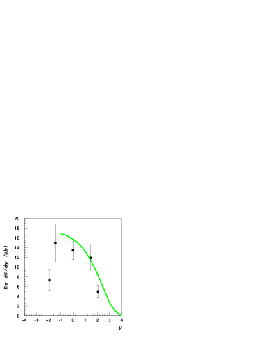
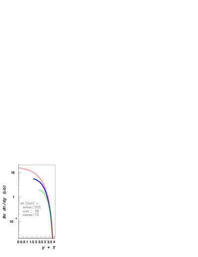
(a)		(b)

Figure 4: Total inelastic cross section for ${J/\Psi}$ production (19) as a function of (a) rapidity $y$, (b) shifted rapidity $y+Y$, where $Y=(1/2)\ln(s^{\prime}/s)$. Data points are taken from Ref. RdeCass .

In Fig. 4(b) we show the “hidden parton scaling” due to the saturation of the nuclear wave function, see Sec. IV.3. We observe an effect similar to the “limiting fragmentation” in the total inclusive cross section. Let us emphasize that such a “hidden parton scaling” is a general feature of all hard processes at high energy in the saturation picture. It is due to the saturation of partons in the nucleus.

In Fig. 5 we show the nuclear modification factor as a function of rapidity and centrality. In agreement with our discussion in Sec. IV $R_{pA}({J/\Psi})$ is suppressed at forward rapidities and enhanced at midrapidity. The functional dependence on rapidity and centrality is given by Eqs. (23),(25). Our results are in a qualitative agreement with the PHENIX data Adler:2005ph ; RdeCass .

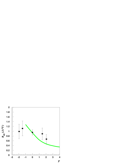
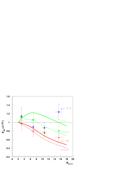
Figure 5: Nuclear modification factor $R_{J/\Psi}$ as a function of (a) rapidity $y$, (b) $N_{\mathrm{coll}}^{Au}$ at different rapidities. Solid lines: numerical calculation. Data points are from Ref. RdeCass .

Finally, in Fig. 6 we present our calculation of the exponent $\alpha$ defined as follows: $\sigma_{pA}=A^{\alpha}\,\sigma_{pp}$. As discussed in Sec. IV.3 we expect an approximate $x_{F}$ scaling at close energies due to the slow dependence of the saturation scale on energy. At smaller $x_{F}$ nuclear absorption plays a significant role; because of formation time effects, it suppresses the ${J/\Psi}$ production at SPS stronger than at Fermilab and contributes towards improving the $x_{F}$ scaling. In the same figure we plot our prediction for LHC. At such high energies the proton’s wave function saturates, which results in the exact $x_{1}$ scaling, as discussed in Sec. IV.3. Thus, in the region $x_{1}\gg x_{2}$ we predict $x_{F}$ scaling of $\alpha$ at energies ${{}_{\displaystyle{>}}\atop\displaystyle{\sim}}5$ TeV.

We would like to draw the reader’s attention to the fact that $\alpha\approx 2/3$ at the highest energy in Fig. 6. This is just the value of $\alpha$ one expects to measure in the collision of two black disks: one of radius $R_{p}$ another of radius $R_{A}$. At LHC energies the absorption starts only at $y\leq-3$. Therefore, from our discussion in Sec. IV.2 we expect that $\alpha$ will approach $4/3$ at $y<0$. This behavior will be best seen in a plot of $\alpha$ as a function of $y$ since the plot versus $x_{F}$ exponentially expands the fragmentation region, while shrinking the interesting central rapidity one.

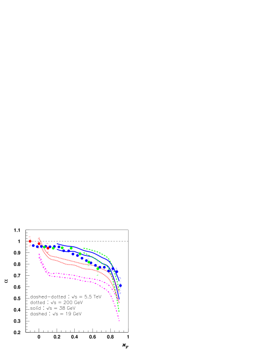
Figure 6: $\alpha$ as a function of $x_{F}$ for different energies. $\alpha$ was extracted by fitting function $A^{\alpha}$ to the calculated $\sigma_{pA}/\sigma_{pp}$. Bands show the uncertainty of the fit.

VI Summary and Conclusions

In this paper we have analyzed the ${J/\Psi}$ production in p(d)A collisions at high energies. We have pointed out that due to the large coherence length associated with the ${J/\Psi}$ production and formation the dominant production mechanism in the case of heavy nuclei is a double-gluon exchange which leads to a significant enhancement of the cross section at backward rapidities. In the case of DIS this effect has been discussed in Ref. HKZ , and the relevant arguments for hard processes at forward rapidities have been given in Brodsky:1991dj . At forward rapidities the ${J/\Psi}$ production is suppressed in much the same way as open charm is KhT . This is due to saturation of gluons in the nuclear wave function, see Fig. 5(b). The transition between the enhancement and the suppression regimes in ${J/\Psi}$ production happens when $Q_{s}\approx M_{\psi}$. Eq. (19) provides an analytical formula for the total cross section of ${J/\Psi}$ production in the region where $\tau_{P}>R_{A}$.

The dominance of the double-gluon exchange mechanism for the case of heavy nuclei has an important implication. It means that ${J/\Psi}$ is produced directly in the color singlet state. A clean way to measure the contribution of the double gluon exchange from different nucleons is to measure ${J/\Psi}$ production in proton–deuteron collisions and to trigger on the final fragmentation state of the deuteron. A signature of the double-gluon exchange mechanism will be the absence of intact nucleons YD . Such an experimental study can shed further light on the problem of ${J/\Psi}$ production.

We have argued that the total ${J/\Psi}$ production cross section exhibits the “hidden parton scaling”, see Fig. 4(b). Owing to the saturation of gluons in the nucleus, the cross section becomes independent of $x_{2}$. Thus it scales with $x_{1}$, or, equivalently, with $y+Y=\ln x_{1}+\mathrm{const.}$ In other words, $d\sigma(x_{1})/dx_{1}$ has a universal shape for different energies.

In Sec. IV.3 we studied the $x_{F}$ scaling phenomenon observed at lower energies. We found that this scaling holds only for close energies since the scaling violating factor is a slow function of energy: $\sim s^{0.25}$. However, at energies as high as LHC energy we expect the saturation of gluons in the proton which will manifests itself in the effective disappearance of the factor $s^{0.25}$ and will result in the exact $x_{1}$ scaling. In turn, an exact $x_{1}$ scaling can be considered as a signature of the saturation in the proton.

- (1) P. Nason, S. Dawson and R. K. Ellis, Nucl. Phys. B 327, 49 (1989) [Erratum-ibid. B 335, 260 (1990)]; P. Nason, S. Dawson and R. K. Ellis, Nucl. Phys. B 303, 607 (1988).
- (2) T. Appelquist and J. Carazzone, Phys. Rev. D 11, 2856 (1975).
- (3) N. Brambilla et al., arXiv:hep-ph/0412158.
- (4) T. Matsui and H. Satz, Phys. Lett. B 178, 416 (1986).
- (5) J. Badier et al. [NA3 Collaboration], Z. Phys. C 20, 101 (1983).
- (6) M. J. Leitch et al. [FNAL E866/NuSea collaboration], Phys. Rev. Lett. 84, 3256 (2000) [arXiv:nucl-ex/9909007].
- (7) S. S. Adler et al. [PHENIX Collaboration], arXiv:nucl-ex/0507032.
- (8) S. J. Brodsky, P. Hoyer, A. H. Mueller and W. K. Tang, Nucl. Phys. B 369, 519 (1992).
- (9) B. Z. Kopeliovich and F. Niedermayer, JINR-E2-84-834
- (10) R. Vogt, S. J. Brodsky and P. Hoyer, Nucl. Phys. B 360, 67 (1991).
- (11) S. Gavin and J. Milana, Phys. Rev. Lett. 68, 1834 (1992).
- (12) D. Kharzeev and H. Satz, Z. Phys. C 60, 389 (1993).
- (13) L. Clavelli, P. H. Cox, B. Harms and S. Jones, Phys. Rev. D 32, 612 (1985).
- (14) C. J. Benesh, J. w. Qiu and J. P. Vary, Phys. Rev. C 50, 1015 (1994) [arXiv:hep-ph/9403265]; J. w. Qiu, J. P. Vary and X. f. Zhang, Phys. Rev. Lett. 88, 232301 (2002) [arXiv:hep-ph/9809442].
- (15) H. Fujii, Prog. Theor. Phys. Suppl. 151, 127 (2003) [arXiv:hep-ph/0303219].
- (16) L. V. Gribov, E. M. Levin and M. G. Ryskin, Phys. Rept. 100, 1 (1983).
- (17) A. H. Mueller and J. w. Qiu, Nucl. Phys. B 268, 427 (1986).
- (18) J. P. Blaizot and A. H. Mueller, Nucl. Phys. B 289, 847 (1987).
- (19) L. D. McLerran and R. Venugopalan, Phys. Rev. D 49, 2233 (1994) [arXiv:hep-ph/9309289], Phys. Rev. D 49, 3352 (1994) [arXiv:hep-ph/9311205], Phys. Rev. D 50, 2225 (1994) [arXiv:hep-ph/9402335], Phys. Rev. D 59, 094002 (1999) [arXiv:hep-ph/9809427].
- (20) D. Kharzeev and K. Tuchin, Nucl. Phys. A 735, 248 (2004) [arXiv:hep-ph/0310358].
- (21) K. Tuchin, arXiv:hep-ph/0401022, arXiv:hep-ph/0402298.
- (22) F. Gelis and R. Venugopalan, Phys. Rev. D 69, 014019 (2004) [arXiv:hep-ph/0310090].
- (23) J. P. Blaizot, F. Gelis and R. Venugopalan, Nucl. Phys. A 743, 57 (2004) [arXiv:hep-ph/0402257].
- (24) F. Gelis, K. Kajantie and T. Lappi, Phys. Rev. C 71, 024904 (2005) [arXiv:hep-ph/0409058].
- (25) H. Fujii, F. Gelis and R. Venugopalan, arXiv:hep-ph/0504047.
- (26) E. M. Levin, M. G. Ryskin, Y. M. Shabelski and A. G. Shuvaev, Sov. J. Nucl. Phys. 53, 657 (1991) [Yad. Fiz. 53, 1059 (1991)].
- (27) V. N. Gribov, B. L. Ioffe and I. Y. Pomeranchuk, Sov. J. Nucl. Phys. 2, 549 (1966) [Yad. Fiz. 2, 768 (1965)]; B. L. Ioffe, Phys. Lett. B 30, 123 (1969).
- (28) D. Kharzeev and H. Satz, Phys. Lett. B 356, 365 (1995) [arXiv:hep-ph/9504397].
- (29) S. J. Brodsky and A. H. Mueller, Phys. Lett. B 206, 685 (1988).
- (30) B. Z. Kopeliovich and B. G. Zakharov, Phys. Rev. D 44, 3466 (1991).
- (31) D. Kharzeev and R. L. Thews, Phys. Rev. C 60, 041901 (1999) [arXiv:nucl-th/9907021].
- (32) N. N. Nikolaev and B. G. Zakharov, Z. Phys. C 49, 607 (1991).
- (33) A. H. Mueller, Nucl. Phys. B 415, 373 (1994).
- (34) Y. V. Kovchegov, Phys. Rev. D 54, 5463 (1996) [arXiv:hep-ph/9605446]; Phys. Rev. D 55, 5445 (1997) [arXiv:hep-ph/9701229].
- (35) J. Hufner, B. Kopeliovich and A. B. Zamolodchikov, Z. Phys. A 357, 113 (1997) [arXiv:nucl-th/9607033].
- (36) V. N. Gribov, SLAC-TRANS-0102
- (37) A. H. Mueller, Nucl. Phys. B 335, 115 (1990);
- (38) J. Kublbeck, H. Eck and R. Mertig, Nucl. Phys. Proc. Suppl. 29A, 204 (1992), http://www.feyncalc.org/.
- (39) B. Z. Kopeliovich, A. V. Tarasov and A. Schafer, Phys. Rev. C 59, 1609 (1999) [arXiv:hep-ph/9808378];
- (40) S. J. Brodsky, L. Frankfurt, J. F. Gunion, A. H. Mueller and M. Strikman, Phys. Rev. D 50, 3134 (1994) [arXiv:hep-ph/9402283].
- (41) M. G. Ryskin, R. G. Roberts, A. D. Martin and E. M. Levin, Z. Phys. C 76, 231 (1997) [arXiv:hep-ph/9511228].
- (42) E. Gotsman, E. Levin, M. Lublinsky, U. Maor and E. Naftali, Acta Phys. Polon. B 34, 3255 (2003).
- (43) D. Kharzeev, C. Lourenco, M. Nardi and H. Satz, Z. Phys. C 74, 307 (1997) [arXiv:hep-ph/9612217].
- (44) D. Kharzeev, E. Levin and M. Nardi, Nucl. Phys. A 730, 448 (2004) [Erratum-ibid. A 743, 329 (2004)] [arXiv:hep-ph/0212316]; Nucl. Phys. A 747, 609 (2005) [arXiv:hep-ph/0408050].
- (45) E. Levin and K. Tuchin, Nucl. Phys. B 573, 833 (2000) [arXiv:hep-ph/9908317], Nucl. Phys. A 693, 787 (2001) [arXiv:hep-ph/0101275].
- (46) K. Golec-Biernat and M. Wüsthoff, Eur. Phys. J. C 20, 313 (2001) [arXiv:hep-ph/0102093], Phys. Rev. D 60, 114023 (1999) [arXiv:hep-ph/9903358], Phys. Rev. D 59, 014017 (1999) [arXiv:hep-ph/9807513].
- (47) D. Kharzeev and M. Nardi, Phys. Lett. B 507, 121 (2001) [arXiv:nucl-th/0012025].
- (48) D. Kharzeev and E. Levin, Phys. Lett. B 523, 79 (2001) [arXiv:nucl-th/0108006].
- (49) D. Kharzeev, E. Levin and L. McLerran, Phys. Lett. B 561, 93 (2003) [arXiv:hep-ph/0210332].
- (50) D. Kharzeev, Y. V. Kovchegov and K. Tuchin, Phys. Rev. D 68, 094013 (2003) [arXiv:hep-ph/0307037].
- (51) D. N. Triantafyllopoulos, Nucl. Phys. B 648, 293 (2003) [arXiv:hep-ph/0209121].
- (52) E. A. Kuraev, L. N. Lipatov and V. S. Fadin, Sov. Phys. JETP 45, 199 (1977) [Zh. Eksp. Teor. Fiz. 72, 377 (1977)]. I. I. Balitsky and L. N. Lipatov, Sov. J. Nucl. Phys. 28, 822 (1978) [Yad. Fiz. 28, 1597 (1978)].
- (53) L. Frankfurt, W. Koepf and M. Strikman, Phys. Rev. D 54, 3194 (1996) [arXiv:hep-ph/9509311]; L. Frankfurt, W. Koepf and M. Strikman, Phys. Rev. D 57, 512 (1998) [arXiv:hep-ph/9702216].
- (54) E. Gotsman, E. Ferreira, E. Levin, U. Maor and E. Naftali, Phys. Lett. B 503, 277 (2001) [arXiv:hep-ph/0101142].
- (55) E. Gotsman, E. Levin, M. Lublinsky, U. Maor, E. Naftali and K. Tuchin, J. Phys. G 27, 2297 (2001) [arXiv:hep-ph/0010198].
- (56) R.G. de Cassagnac (PHENIX Collaboration), talk at “Quark Matter” 2004, Oakland, California, January 12–17, 2004.
- (57) This argument is due to Yuri Dokshitzer.