Neutrino emission and cooling rates of spin-one color superconductors

Abstract

Neutrino emissivities due to direct Urca processes of several spin-one color-superconducting phases of dense quark matter are calculated. In particular, the role of anisotropies and nodes of the gap functions is analyzed. Results for the specific heat as well as for the cooling rates of the color-spin-locked, planar, polar, and A phases are presented and consequences for the physics of neutron stars are briefly discussed. Furthermore, it is shown that the A phase exhibits a helicity order, giving rise to a reflection asymmetry in the neutrino emissivity.

I Introduction

Exotic states of matter are expected to exist in the central regions of compact stars. The baryon density in these systems is likely to exceed several times the nuclear saturation density, $\rho_{0}\simeq 0.15~{}\mbox{fm}^{-3}$. The exact nature of such dense matter, however, is yet unknown. It was suggested already 30 years ago perry that it might be deconfined quark matter. Since the temperatures in neutron stars are sufficiently low, this matter is likely to be in a color-superconducting state. (For reviews on color superconductivity see Refs. reviews .) There is little doubt that dense baryonic matter at asymptotically high quark chemical potential $\mu$ is a color superconductor bailin . In this case, the ground state is the color-flavor locked (CFL) phase alford (for studies of the CFL phase in QCD at asymptotic density, see also Refs. weak-cfl1 ; weak-cfl2 ). At densities existing in stars, however, this phase may not necessarily be realized. The main reason for the potential breakdown of the CFL phase is a relatively large difference between the masses of the strange quark, $m_{s}$, and the masses of the up and down quarks, $m_{u}\simeq m_{d}$, which is negligible only at large densities. This difference, together with the requirements of $\beta$ equilibrium and electric and color charge neutrality, gives rise to a mismatch between the Fermi momenta of the quarks that form Cooper pairs neutrality . Therefore, the conventional BCS pairing bcs , which is the underlying mechanism of the CFL state, becomes questionable and the search for the true ground state of quark matter in compact stars has to include different, unconventional superconducting states shovkovy ; gCFL ; cfl+mesons ; alford2 .

Determining the ground state of QCD at moderate densities from first principles, i.e., within the framework of QCD, is not possible at present. It is natural therefore to make use of astrophysical observations to test the presence of various suggested phases. The goal of this paper is to investigate color superconductors in which quarks of the same flavor form Cooper pairs and to study their effect on specific observables.

Single-flavor Cooper pairing is the simplest possibility for neutral quark matter. Contrary to other unconventional pairing mechanisms, such as the gapless 2SC phase shovkovy , the gapless CFL phase gCFL , the CFL phase with additional meson condensates cfl+mesons , or the crystalline phases alford2 , it is allowed for arbitrarily large mismatches between the Fermi momenta of different quark flavors. Single-flavor pairing in the color anti-triplet channel is possible only in the symmetric spin-one channel bailin ; spin1 ; schaefer ; Schmitt:2002sc ; Schmitt:2003xq ; andreas . This is the consequence of the Pauli principle which requires the wave function of the Cooper pair to be antisymmetric under the exchange of the constituent quarks. This is in contrast to pairing of different flavors where the antisymmetric spin-zero channel is allowed.

Furnishing triplet representations with respect to both color and spin groups, the order parameter in a spin-one color superconductor is given by a complex 3$\times$3 matrix. This is similar to superfluid ³He, where condensation occurs in spin and angular momentum triplets vollhardt . In both systems, the matrix structure of the order parameter gives rise to several possible phases. In ³He the observed phases are the so-called A, B, and $A_{1}$ phases. In this paper, we consider the following four main spin-one color-superconducting phases of quark matter: the color-spin locked (CSL), planar, polar, and A phases, proposed in Refs. schaefer ; Schmitt:2002sc ; Schmitt:2003xq ; andreas ; Buballa:2002wy . The A and CSL phases are analogues of the A and B phases in ³He, respectively.

In contrast to the nonrelativistic case of ³He, spin-one color-superconductors may involve pairing of quarks of the same as well as of opposite chiralities. In this paper, we focus on the so-called “transverse” phases, in which exclusively quarks of opposite chiralities pair. Theoretical studies at asymptotically large densities suggest that these phases are preferred schaefer ; andreas .

As in the case of ³He, the gap functions of most of the quark phases considered here are anisotropic in momentum space. Only the CSL phase is isotropic. The gap in the polar phase vanishes at the south and north poles of the Fermi sphere, whereas the gap in the planar phase is anisotropic but nonzero in any direction of the quasiparticle momentum. The A phase is special in the sense that it has two gapped quasiparticle modes with different angular structures, one of which has two point nodes.

One should expect that the anisotropies and especially the nodes affect the physical properties of the corresponding quark phases. The low energy excitations around the nodes give important contributions to various thermodynamical and transport properties, e.g., the specific heat, the neutrino emissivity, the viscosity, the heat and electrical conductivity, etc. In application to compact stars, the specific heat and the neutrino emissivity determine the cooling behavior during the first $10^{5}$ – $10^{6}$ years of the stellar evolution. In this paper, we compute these two quantities for the four mentioned spin-one color-superconducting phases and deduce the resulting cooling rates. In addition, we will discuss the reason why the distribution of neutrino emission from the A phase breaks reflection symmetry in position space.

The paper is organized as follows. The general formalism of calculating the time derivative of the neutrino distribution function is given in Sec. II. The main result from Sec. II is then used in Sec. III to compute the neutrino emissivity. The specific heat is calculated in Sec. IV. Both quantities are used in Sec. V to discuss the cooling behavior of the considered phases. In Sec. VI we explain the asymmetry of the neutrino emission in the A phase. Finally, we comment briefly on the effect of nonzero quark masses in Sec. VII.

Our convention for the metric tensor is $g^{\mu\nu}=\mbox{diag}(1,-1,-1,-1)$. Our units are $\hbar=c=k_{B}=1$. Four-vectors are denoted by capital letters, $K\equiv K^{\mu}=(k_{0},{\bf k})$, while $k\equiv|{\bf k}|$ and $\hat{\mathbf{k}}\equiv{\bf k}/k$. We work in the imaginary-time formalism, i.e., $T/V\sum_{K}\equiv T\sum_{n}\int d^{3}{\bf k}/(2\pi)^{3}$, where $n$ labels the Matsubara frequencies $\omega_{n}\equiv ik_{0}$. The Matsubara frequencies are $\omega_{n}\equiv 2n\pi T$ for bosons, and $\omega_{n}\equiv(2n+1)\pi T$ for fermions.

II Time derivative of the neutrino distribution function

In this section, we derive a general expression for the time derivative of the neutrino distribution function in spin-one color-superconducting phases.

II.1 General formalism

Within the Kadanoff-Baym formalism KB , one derives the following kinetic equation for the neutrino Green function (see for example Refs. VoskSen ; friman ; kadanoff ):

$$i\partial_{X}^{\lambda}\mbox{Tr}[\gamma_{\lambda}G^{<}_{\nu}(X,P_{\nu})]=-\mbox{Tr}\left[G^{>}_{\nu}(X,P_{\nu})\Sigma^{<}_{\nu}(X,P_{\nu})-\Sigma^{>}_{\nu}(X,P_{\nu})G^{<}_{\nu}(X,P_{\nu})\right]\,\,,$$ (1)

where the trace runs over Dirac space. (Here and in the following, the index $\nu$ always labels neutrino quantities and should not be confused with a Lorentz index.) The kinetic equation is obtained from the general Kadanoff-Baym equation after applying a gradient expansion, which is valid when the neutrino Green functions $G^{<,>}_{\nu}(X,P_{\nu})$ and self-energies $\Sigma^{<,>}_{\nu}(X,P_{\nu})$ are slowly varying functions of the space-time coordinate $X=(t,\mathbf{x})$. For our purposes, it is sufficient to consider spatially homogeneous systems which are close to equilibrium. In this case, the neutrino Green functions assume the following approximate form friman :

$$iG^{<}_{\nu}(t,P_{\nu}) = -(\gamma^{\lambda}P_{\nu,\lambda}+\mu_{\nu}\gamma_{0})\frac{\pi}{p_{\nu}}\left\{f_{\nu}(t,\mathbf{p}_{\nu})\,\delta(p_{\nu 0}+\mu_{\nu}-p_{\nu})-[1-f_{\overline{\nu}}(t,-\mathbf{p}_{\nu})]\,\delta(p_{\nu 0}+\mu_{\nu}+p_{\nu})\right\}\,,$$ (2a)

$$iG^{>}_{\nu}(t,P_{\nu}) = (\gamma^{\lambda}P_{\nu,\lambda}+\mu_{\nu}\gamma_{0})\frac{\pi}{p_{\nu}}\left\{[1-f_{\nu}(t,\mathbf{p}_{\nu})]\,\delta(p_{\nu 0}+\mu_{\nu}-p_{\nu})-f_{\overline{\nu}}(t,-\mathbf{p}_{\nu})\,\delta(p_{\nu 0}+\mu_{\nu}+p_{\nu})\right\}\,,$$ (2b)

where $\mu_{\nu}$ is the neutrino chemical potential. The functions $f_{\nu,\overline{\nu}}(t,\mathbf{p}_{\nu})$ are the neutrino and antineutrino distribution functions. We are interested in the Urca processes $u+e^{-}\to d+\nu$ (electron capture) and $d\to u+e^{-}+\overline{\nu}$ ($\beta$-decay), which provide the dominant cooling mechanism for quark matter. These processes are important for neutron stars with core temperatures of the order of or smaller than several MeV. In this stage of the stellar evolution, the mean free path of neutrinos becomes larger than the stellar radius, wherefore in our results we shall set $\mu_{\nu}=0$.

The leading order contributions to the neutrino self-energies which enter the kinetic equation (1) are given by the diagrams in Fig. 1. For the sake of simplicity, we do not take strange quarks into account. Their weak interactions are Cabibbo suppressed, and their number density is not expected to be very large. (Admittedly, however, the bigger phase space for the Urca processes involving massive strange quarks may partially compensate this suppression.) The diagrams in Fig. 1 translate into the following expressions,

$$\Sigma_{\nu}^{<}(t,P_{\nu}) = \frac{G_{F}^{2}}{2}\int\frac{d^{4}P_{e}}{(2\pi)^{4}}\gamma^{\lambda}(1-\gamma_{5})(\gamma^{\kappa}P_{e,\kappa}+\mu_{e}\gamma_{0})\gamma^{\sigma}(1-\gamma_{5})$$ (3a)

$$\times\;\Pi_{\lambda\sigma}^{>}(P_{e}-P_{\nu})\frac{\pi}{p_{e}}f_{e}(t,\mathbf{p}_{e})\delta(p_{e0}+\mu_{e}-p_{e}),$$

$$\Sigma_{\nu}^{>}(t,P_{\nu}) = -\frac{G_{F}^{2}}{2}\int\frac{d^{4}P_{e}}{(2\pi)^{4}}\gamma^{\lambda}(1-\gamma_{5})(\gamma^{\kappa}P_{e,\kappa}+\mu_{e}\gamma_{0})\gamma^{\sigma}(1-\gamma_{5})$$ (3b)

$$\times\;\Pi_{\lambda\sigma}^{<}(P_{e}-P_{\nu})\frac{\pi}{p_{e}}[1-f_{e}(t,\mathbf{p}_{e})]\delta(p_{e0}+\mu_{e}-p_{e}),$$

where $G_{F}$ is the Fermi coupling constant and $\mu_{e}$ is the electron chemical potential. In the derivation we used the explicit form of the electron Green functions $G^{<,>}_{e}(t,P_{e})$. They are given by expressions analogous to Eqs. (2). We have neglected the positron contribution, i.e., the analogues of the second terms in curly brackets on the right-hand sides of Eqs. (2). [Note that the processes involving positrons, $u\to d+e^{+}+\nu$ and $d+e^{+}\to u+\overline{\nu}$, are suppressed by a large factor $\exp(2\mu_{e}/T)$ because $\mu_{e}$ is positive and, in the regime under consideration, much larger than the temperature.]

The functions $\Pi_{\lambda\sigma}^{<,>}(P_{e}-P_{\nu})$ are the self-energies of the $W$ bosons. The $W$ exchange is approximated by its local form since the typical neutrino energies are much smaller than the $W$ mass. In the case of neutrino processes in compact stars, the corresponding neutrino energies do not exceed several dozens MeV.

Figure 1: Neutrino self-energies relevant for the neutrino Urca processes in the close-time-path formalism. The $+$ and $-$ signs assign the vertices to the upper and lower branch of the time contour, respectively.

Next, we insert the Green functions (2) and self-energies (3) into the kinetic equation (1). In order to obtain the expression for the neutrino (antineutrino) distribution function, we integrate on both sides of the kinetic equation over $p_{\nu 0}$ from $-\mu_{\nu}$ to $\infty$ (from $-\infty$ to $-\mu_{\nu}$). The results are

$$\frac{\partial}{\partial t}f_{\nu}(t,\mathbf{p}_{\nu}) = -i\frac{G_{F}^{2}}{16}\int\frac{d^{3}\mathbf{p}_{e}}{(2\pi)^{3}p_{\nu}p_{e}}L^{\lambda\sigma}({\bf p}_{e},{\bf p}_{\nu})\,\left\{[1-f_{\nu}(t,\mathbf{p}_{\nu})]\,f_{e}(t,\mathbf{p}_{e})\,\Pi_{\lambda\sigma}^{>}(Q)\right.$$ (4a)

$$\left.\hskip 142.26378pt-\;f_{\nu}(t,\mathbf{p}_{\nu})\,[1-f_{e}(t,\mathbf{p}_{e})]\,\Pi_{\lambda\sigma}^{<}(Q)\right\}\,\,,$$

$$\frac{\partial}{\partial t}f_{\overline{\nu}}(t,\mathbf{p}_{\nu}) = -i\frac{G_{F}^{2}}{16}\int\frac{d^{3}\mathbf{p}_{e}}{(2\pi)^{3}p_{\nu}p_{e}}L^{\lambda\sigma}({\bf p}_{e},{\bf p}_{\nu})\,\left\{[1-f_{\overline{\nu}}(t,\mathbf{p}_{\nu})]\,[1-f_{e}(t,\mathbf{p}_{e})]\,\Pi_{\lambda\sigma}^{<}(Q^{\prime})\right.$$ (4b)

$$\left.\hskip 142.26378pt-\;f_{\overline{\nu}}(t,\mathbf{p}_{\nu})\,f_{e}(t,\mathbf{p}_{e})\,\Pi_{\lambda\sigma}^{>}(Q^{\prime})\right\}\,\,,$$

with the four-momenta $Q\equiv(p_{e}-p_{\nu}-\mu_{e}+\mu_{\nu},{\bf p}_{e}-{\bf p}_{\nu})$ and $Q^{\prime}\equiv(p_{e}+p_{\nu}-\mu_{e}+\mu_{\nu},{\bf p}_{e}+{\bf p}_{\nu})$, and the shorthand notation

$$L^{\lambda\sigma}({\bf p}_{e},{\bf p}_{\nu})\equiv\mbox{Tr}\left[(\gamma_{0}p_{e}-\bm{\gamma}\cdot{\bf p}_{e})\,\gamma^{\sigma}(1-\gamma^{5})(\gamma_{0}p_{\nu}-\bm{\gamma}\cdot{\bf p}_{\nu})\,\gamma^{\lambda}(1-\gamma^{5})\right].$$ (5)

In the following, it is convenient to express the results in terms of the retarded self-energy for $W$ bosons, $\Pi^{\lambda\sigma}_{R}$. Therefore, we shall use the following relations:

$$\Pi^{>}(Q) = -2i[1+n_{B}(q_{0})]\mbox{Im}\Pi_{R}(Q)\,\,,$$ (6a)

$$\Pi^{<}(Q) = -2i\,n_{B}(q_{0})\mbox{Im}\Pi_{R}(Q)\,\,,$$ (6b)

where $n_{B}(\omega)\equiv 1/(e^{\omega/T}-1)$ is the Bose-Einstein distribution function.

Here we consider the cooling of quark matter only in the absence of neutrino trapping. Then, the neutrino and antineutrino distribution functions on the right-hand side of Eq. (4) are vanishing, $f_{\nu,\overline{\nu}}(t,\mathbf{p}_{\nu})=0$. The electron distribution function can be approximated by its equilibrium expression,

$$f_{e}(t,\mathbf{p}_{e})\simeq n_{F}(p_{e}-\mu_{e})\,\,,$$ (7)

with $n_{F}(\omega)\equiv 1/(e^{\omega/T}+1)$. Then, one arrives at

$$\frac{\partial}{\partial t}f_{\nu}(t,\mathbf{p}_{\nu}) = \frac{G_{F}^{2}}{8}\int\frac{d^{3}\mathbf{p}_{e}}{(2\pi)^{3}p_{\nu}p_{e}}L_{\lambda\sigma}({\bf p}_{e},{\bf p}_{\nu})\,n_{F}(p_{e}-\mu_{e})\,n_{B}(p_{\nu}+\mu_{e}-p_{e})\,\mathrm{Im}\Pi_{R}^{\lambda\sigma}(Q),$$ (8a)

$$\frac{\partial}{\partial t}f_{\overline{\nu}}(t,\mathbf{p}_{\nu}) = -\frac{G_{F}^{2}}{8}\int\frac{d^{3}\mathbf{p}_{e}}{(2\pi)^{3}p_{\nu}p_{e}}L_{\lambda\sigma}({\bf p}_{e},{\bf p}_{\nu})\,n_{F}(\mu_{e}-p_{e})\,n_{B}(p_{\nu}-\mu_{e}+p_{e})\,\mathrm{Im}\Pi_{R}^{\lambda\sigma}(Q^{\prime}).$$ (8b)

We shall see in Sec. II.4 that the right-hand sides of Eqs. (8a) and (8b) are in fact identical.

II.2 Quark propagators in spin-one color superconductors

As we shall see below, cf. Eq. (18), the expression for the imaginary part of the polarization tensor of the W-vector boson is given in terms of the quark propagator $S(K)$. In this paper, we consider the following four spin-one superconducting phases: the CSL, planar, polar, and A phases. Each of these phases is characterized by a $12\times 12$ gap matrix ${\cal M}_{\bf k}$ in color and Dirac space,

$${\cal M}_{\bf k}=\sum_{i,j=1}^{3}J_{i}\Delta_{ij}\gamma_{\perp,j}(\hat{\mathbf{k}})\,\,,$$ (9)

where $(J_{i})_{jk}=-i\epsilon_{ijk}$ and $\bm{\gamma}_{\perp}(\hat{\mathbf{k}})\equiv\bm{\gamma}-\hat{\mathbf{k}}\,\bm{\gamma}\cdot\hat{\mathbf{k}}$ are basis vectors for the color antitriplet and spin triplet representations, respectively. We focus exclusively on the transverse phases, which have the highest pressure at asymptotic density and thus are expected to be preferred over others. For a more general form of the matrix ${\cal M}_{\bf k}$ see Ref. andreas . The matrix $\Delta$ is a complex $3\times 3$ matrix and assumes a specific structure for each of the phases. In Table 1, we give $\Delta$ and the resulting matrices ${\cal M}_{\bf k}$.

phase	$\Delta_{ij}$	${\cal M}_{\bf k}$	$\lambda_{{\bf k},1}\;(n_{1})$	$\lambda_{{\bf k},2}\;(n_{2})$	$\lambda_{{\bf k},3}\;(n_{3})$
CSL	$\delta_{ij}$	${\bf J}\cdot\bm{\gamma}_{\perp}(\hat{\mathbf{k}})$	2 (8)	0 (4)	–
planar	$\delta_{i1}\delta_{j1}+\delta_{i2}\delta_{j2}$	$J_{1}\gamma_{\perp,1}(\hat{\mathbf{k}})+J_{2}\gamma_{\perp,2}(\hat{\mathbf{k}})$	$1+\cos^{2}\theta_{\bf k}\;(8)$	0 (4)	–
polar	$\delta_{i3}\delta_{j3}$	$J_{3}\gamma_{\perp,3}(\hat{\mathbf{k}})$	$\sin^{2}\theta_{\bf k}\;(8)$	0 (4)	–
A	$\delta_{i3}(\delta_{j1}+i\,\delta_{j2})$	$J_{3}[\gamma_{\perp,1}(\hat{\mathbf{k}})+i\,\gamma_{\perp,2}(\hat{\mathbf{k}})]$	$(1+|\cos\theta_{\bf k}|)^{2}\;(4)$	$(1-|\cos\theta_{\bf k}|)^{2}\;(4)$	0  (4)

Table 1: Matrices $\Delta$ and ${\cal M}_{\bf k}$ and eigenvalues $\lambda_{{\bf k},r}$ with corresponding degeneracies $n_{r}$ for four spin-one color superconductors. The angle between ${\bf k}$ and the $z$-axis is denoted by $\theta_{\bf k}$.

In spin-one color superconductors, the quark propagator is diagonal in flavor space, $S(K)={\rm diag}[S_{u}(K),S_{d}(K)]$. The Nambu-Gorkov structure of the flavor-diagonal elements is given by

$$S_{f}(K)=\left(\begin{array}[]{cc}G_{f}^{+}(K)&\Xi_{f}^{-}(K)\\ \Xi_{f}^{+}(K)&G_{f}^{-}(K)\end{array}\right)\,\,,\qquad f=u,d\,\,,$$ (10)

where Schmitt:2002sc ; Schmitt:2003xq ; andreas

$$G^{\pm}_{f}(K)=\left[G_{0,f}^{\mp}(K)\right]^{-1}\,\sum_{e,r}\frac{{\cal P}_{{\bf k},r}^{\pm}\,\Lambda_{\bf k}^{\mp e}}{k_{0}^{2}-(\epsilon_{{\bf k},r,f}^{e})^{2}}\,\,.$$ (11)

For the sake of simplicity, we have not included the quark self-energy correction. For a more general expression of the propagator, including this correction, see Refs. Brown:2000eh ; Wang:2001aq . The inverse free propagator for quarks and charge-conjugate quarks in the ultrarelativistic limit is

$$\left[G_{0,f}^{\pm}(K)\right]^{-1}=\gamma^{\mu}K_{\mu}\pm\mu_{f}\gamma_{0}=\gamma_{0}\sum_{e}[k_{0}\pm(\mu_{f}-ek)]\,\Lambda_{\bf k}^{\pm e}\,\,.$$ (12)

The Dirac matrices $\Lambda_{\bf k}^{e}\equiv(1+e\gamma_{0}\bm{\gamma}\cdot\hat{\mathbf{k}})/2$, where $e=\pm$, are projectors onto positive and negative energy states. The matrices ${\cal P}_{{\bf k},r}^{-}$ and ${\cal P}_{{\bf k},r}^{+}$ in Eq. (11) are projectors onto the eigenspaces of the matrices ${\cal M}_{\bf k}{\cal M}^{\dagger}_{\bf k}$ and $\gamma^{0}{\cal M}^{\dagger}_{\bf k}{\cal M}_{\bf k}\gamma^{0}$, respectively. Both matrices have the same set of eigenvalues $\lambda_{{\bf k},r}$,

$${\cal M}_{\bf k}{\cal M}^{\dagger}_{\bf k} \equiv \sum_{r}\lambda_{{\bf k},r}{\cal P}_{{\bf k},r}^{-}\,\,,$$ (13)

$$\gamma^{0}{\cal M}^{\dagger}_{\bf k}{\cal M}_{\bf k}\gamma^{0} \equiv \sum_{r}\lambda_{{\bf k},r}{\cal P}_{{\bf k},r}^{+}\,\,.$$ (14)

As we shall see, only the projection operators ${\cal P}_{{\bf k},r}^{+}$ (and not ${\cal P}_{{\bf k},r}^{-}$) are needed in the calculation of the neutrino emission. They are given explicitly in Appendix B. The eigenvalues $\lambda_{{\bf k},r}$ appear in the quasiparticle dispersion relations,

$$\epsilon_{{\bf k},r,f}^{e}=\sqrt{(ek-\mu_{f})^{2}+\lambda_{{\bf k},r}|\phi_{f}|^{2}}\,\,.$$ (15)

Here $\phi_{f}$ are the gap parameters, which are different for $u$ and $d$ quarks in general. The eigenvalues for the four considered phases as well as their degeneracies $n_{r}$ are listed in Table 1. Note that all phases contain an ungapped mode, $\lambda_{{\bf k},2(3)}=0$.

The off-diagonal elements on the right-hand side of Eq. (10) are the so-called anomalous propagators. They are given by

$$\Xi^{+}_{f}(K) = -\sum_{e,r}\gamma_{0}\,{\cal M}_{\bf k}\,\gamma_{0}\,{\cal P}_{{\bf k},r}^{+}\Lambda_{\bf k}^{-e}\,\frac{\phi_{f}}{k_{0}^{2}-(\epsilon_{{\bf k},r,f}^{e})^{2}}\,\,,$$ (16a)

$$\Xi^{-}_{f}(K) = -\sum_{e,r}{\cal M}_{\bf k}^{\dagger}\,{\cal P}_{{\bf k},r}^{-}\Lambda_{\bf k}^{e}\,\frac{\phi^{*}_{f}}{k_{0}^{2}-(\epsilon_{{\bf k},r,f}^{e})^{2}}\,\,.$$ (16b)

The propagators in Eq. (11) have particle and hole type poles at $k_{0}=\pm\epsilon_{{\bf k},r,f}^{+}$, as well as the corresponding antiparticle poles at $k_{0}=\pm\epsilon_{{\bf k},r,f}^{-}$. In the calculation of the imaginary part of the retarded self-energy $\Pi^{\lambda\sigma}_{R}(Q)$, the antiparticle contributions are suppressed by inverse powers of the quark chemical potential. [Note, however, that taking antiparticles into account is important in the calculation of $\mbox{Re}\Pi^{\lambda\sigma}_{R}(Q)$.] In our calculation, therefore, we omit the terms with $e=-$ in the quark propagator and arrive at the following approximate form

$$G^{\pm}_{f}(K)\simeq\gamma_{0}\,\Lambda_{\bf k}^{\mp}\,\sum_{r}{\cal P}_{{\bf k},r}^{\pm}\,\frac{k_{0}\mp(\mu_{f}-k)}{k_{0}^{2}-\epsilon_{{\bf k},r,f}^{2}}\,\,,$$ (17)

where we denoted $\epsilon_{{\bf k},r,f}\equiv\epsilon_{{\bf k},r,f}^{+}$.

II.3 Imaginary part of the W-boson polarization tensor

In this subsection, we evaluate $\mathrm{Im}\Pi_{R}^{\lambda\sigma}$. As can be seen from Fig. 1, the $W$-boson polarization tensor can be written as

$$\Pi^{\lambda\sigma}(Q) \equiv \frac{T}{V}\sum_{K}{\rm Tr}[\Gamma_{-}^{\lambda}\,S(K)\,\Gamma_{+}^{\sigma}\,S(K+Q)]\,\,,$$ (18)

where the trace runs over Nambu-Gorkov, color, flavor, and Dirac space. The 2$\times$2 Nambu-Gorkov structure of the vertices reads

$$\Gamma^{\lambda}_{\pm}=\left(\begin{array}[]{@{\extracolsep{2mm}}cc}\gamma^{\lambda}(1-\gamma^{5})\,\tau_{\pm}&0\\ 0&-\gamma^{\lambda}(1+\gamma^{5})\,\tau_{\mp}\end{array}\right)\,,$$ (19)

where $\tau_{\pm}\equiv(\tau_{1}\pm i\tau_{2})/2$ are matrices in flavor space, constructed from the Pauli matrices $\tau_{1}$, $\tau_{2}$. After performing the traces over Nambu-Gorkov and flavor space,

$$\Pi^{\lambda\sigma}(Q)=\frac{T}{V}\sum_{K}\left\{{\rm Tr}[\gamma^{\lambda}(1-\gamma^{5})\,G_{u}^{+}(K)\,\gamma^{\sigma}(1-\gamma^{5})\,G^{+}_{d}(P)]+{\rm Tr}[\gamma^{\lambda}(1+\gamma^{5})\,G_{d}^{-}(K)\,\gamma^{\sigma}(1+\gamma^{5})\,G^{-}_{u}(P)]\right\}\,\,,$$ (20)

where $P\equiv K+Q$, and the traces run over color and Dirac space. As we see, the anomalous propagators $\Xi^{\pm}_{f}$ do not contribute to the self-energy. This is in contrast to spin-zero color superconductors, such as the (gapless) 2SC and CFL phases, in which the anomalous propagators are off-diagonal in flavor space. In fact, this difference is related to the conservation of electric charge in the diagrams in Fig. 1. The anomalous propagators contain the Cooper pair condensate, which, in the case of a spin-one color superconductor, is of the form $\langle uu\rangle$ or $\langle dd\rangle$. Therefore, the appearance of the anomalous propagators in the diagrams of Fig. 1 is forbidden by electric charge conservation. In a spin-zero color superconductor, however, the condensate is of the form $\langle ud\rangle$. Hence, electric charge can be extracted from or deposited into the condensate of Cooper pairs in the ground state and diagrams containing the anomalous propagators contribute to the $W$-boson polarization tensor jaikumar .

After inserting Eq. (17) into Eq. (20), one arrives at the following expression for the imaginary part,

$${\rm Im}\Pi^{\lambda\sigma}_{R}(Q)=\frac{T}{V}{\rm Im}\,\sum_{K}\sum_{r,s}\left\{\frac{[k_{0}-(\mu_{u}-k)]\,[p_{0}-(\mu_{d}-p)]}{(k_{0}^{2}-\epsilon_{{\bf k},r,u}^{2})\,(p_{0}^{2}-\epsilon_{{\bf p},s,d}^{2})}\,{\cal T}_{rs,+}^{\lambda\sigma}(\hat{\mathbf{k}},\hat{\mathbf{p}})+\frac{[k_{0}+(\mu_{d}-k)]\,[p_{0}+(\mu_{u}-p)]}{(k_{0}^{2}-\epsilon_{{\bf k},r,d}^{2})\,(p_{0}^{2}-\epsilon_{{\bf p},s,u}^{2})}\,{\cal T}_{rs,-}^{\lambda\sigma}(\hat{\mathbf{k}},\hat{\mathbf{p}})\right\},$$ (21)

where we defined the following traces in color and Dirac space,

$${\cal T}_{rs,\pm}^{\lambda\sigma}(\hat{\mathbf{k}},\hat{\mathbf{p}})\equiv{\rm Tr}\left[\gamma^{\lambda}(1\mp\gamma^{5})\,\gamma^{0}\,{\cal P}_{{\bf k},r}^{\pm}\,\Lambda_{\bf k}^{\mp}\,\gamma^{\sigma}(1\mp\gamma^{5})\,\gamma^{0}\,{\cal P}_{{\bf p},s}^{\pm}\,\Lambda_{\bf p}^{\mp}\right]\,\,.$$ (22)

In order to perform the Matsubara sum, we use Eq. (71) in Appendix A. Then, extracting the imaginary part yields

$${\rm Im}\Pi^{\lambda\sigma}_{R}(Q) = -\pi\sum_{r,s}\sum_{e_{1},e_{2}=\pm}\int\frac{d^{3}{\bf k}}{(2\pi)^{3}}\left[{\cal T}_{rs,+}^{\lambda\sigma}(\hat{\mathbf{k}},\hat{\mathbf{p}})\,B_{{\bf k},r,u}^{e_{1}}\,B_{{\bf p},s,d}^{e_{2}}\,\frac{n_{F}(-e_{1}\epsilon_{{\bf k},r,u})\,n_{F}(e_{2}\epsilon_{{\bf p},s,d})}{n_{B}(-e_{1}\epsilon_{{\bf k},r,u}+e_{2}\epsilon_{{\bf p},s,d})}\,\delta(q_{0}-e_{1}\epsilon_{{\bf k},r,u}+e_{2}\epsilon_{{\bf p},s,d})\right.$$ (23)

$$\left.+\;{\cal T}_{rs,-}^{\lambda\sigma}(\hat{\mathbf{k}},\hat{\mathbf{p}})\,B_{{\bf k},r,d}^{e_{1}}\,B_{{\bf p},s,u}^{e_{2}}\,\frac{n_{F}(e_{1}\epsilon_{{\bf k},r,d})\,n_{F}(-e_{2}\epsilon_{{\bf p},s,u})}{n_{B}(e_{1}\epsilon_{{\bf k},r,d}-e_{2}\epsilon_{{\bf p},s,u})}\,\delta(q_{0}+e_{1}\epsilon_{{\bf k},r,d}-e_{2}\epsilon_{{\bf p},s,u})\right]\,\,.$$

Here, we defined the Bogoliubov coefficients

$$B_{{\bf k},r,f}^{e}\equiv\frac{\epsilon_{{\bf k},r,f}+e\,(\mu_{f}-k)}{2\epsilon_{{\bf k},r,f}}\,\,,\qquad(f=u,d\,\,,\quad e=\pm)\,\,.$$ (24)

The two terms on the right-hand side of Eq. (23) yield the same contribution. The physical reason for this is that the second term is just the charge-conjugate counterpart of the first term. The formal proof goes as follows. In the second term, one changes the summation indices $e_{1}\leftrightarrow e_{2}$ and $r\leftrightarrow s$. Then, one introduces the new integration variable ${\bf k}\to-{\bf k}-{\bf q}$ and uses

$${\cal T}_{sr,-}^{\lambda\sigma}(-\hat{\mathbf{p}},-\hat{\mathbf{k}})={\cal T}_{rs,+}^{\lambda\sigma}(\hat{\mathbf{k}},\hat{\mathbf{p}})\,\,,$$ (25)

which holds for all phases considered in this paper. After taking into account that $\lambda_{{\bf k},r}=\lambda_{-{\bf k},r}$, one obtains the first term in Eq. (23). Consequently, in the following we keep only the first term and double the result,

$${\rm Im}\Pi^{\lambda\sigma}_{R}(Q) = -2\pi\sum_{r,s}\sum_{e_{1},e_{2}=\pm}\int\frac{d^{3}{\bf k}}{(2\pi)^{3}}{\cal T}_{rs,+}^{\lambda\sigma}(\hat{\mathbf{k}},\hat{\mathbf{p}})\,B_{{\bf k},r,u}^{e_{1}}\,B_{{\bf p},s,d}^{e_{2}}$$ (26)

$$\times\,\frac{n_{F}(-e_{1}\epsilon_{{\bf k},r,u})\,n_{F}(e_{2}\epsilon_{{\bf p},s,d})}{n_{B}(-e_{1}\epsilon_{{\bf k},r,u}+e_{2}\epsilon_{{\bf p},s,d})}\,\delta(q_{0}-e_{1}\epsilon_{{\bf k},r,u}+e_{2}\epsilon_{{\bf p},s,d})\,\,.$$

The same result may also be written in another form which is more convenient for the use in Eq. (8b), i.e.,

$${\rm Im}\Pi^{\lambda\sigma}_{R}(Q^{\prime}) = 2\pi\sum_{r,s}\sum_{e_{1},e_{2}=\pm}\int\frac{d^{3}{\bf k}}{(2\pi)^{3}}{\cal T}_{rs,+}^{\lambda\sigma}(\hat{\mathbf{k}},\hat{\mathbf{p}}^{\prime})\,B_{{\bf k},r,u}^{e_{1}}\,B_{{\bf p}^{\prime},s,d}^{e_{2}}$$ (27)

$$\times\,\frac{n_{F}(e_{1}\epsilon_{{\bf k},r,u})\,n_{F}(-e_{2}\epsilon_{{\bf p}^{\prime},s,d})}{n_{B}(e_{1}\epsilon_{{\bf k},r,u}-e_{2}\epsilon_{{\bf p}^{\prime},s,d})}\,\delta(q^{\prime}_{0}-e_{1}\epsilon_{{\bf k},r,u}+e_{2}\epsilon_{{\bf p}^{\prime},s,d})\,\,.$$

where we have used Eq. (69) and defined $P^{\prime}\equiv K+Q^{\prime}$.

II.4 General result for the time derivative of the neutrino distribution function

We now insert the results for the polarization tensors (26) and (27) into Eqs. (8a) and (8b), respectively. In order to calculate $L_{\lambda\sigma}({\bf p}_{e},{\bf p}_{\nu})\,{\rm Im}\Pi_{R}^{\lambda\sigma}(Q)$, we have to compute the contraction of the tensor $L_{\lambda\sigma}({\bf p}_{e},{\bf p}_{\nu})$ with the color-Dirac trace ${\cal T}_{rs,+}^{\lambda\sigma}(\hat{\mathbf{k}},\hat{\mathbf{p}})$. In all cases considered in this paper, we can write the result as

$$L_{\lambda\sigma}({\bf p}_{e},{\bf p}_{\nu})\,{\cal T}_{rs,+}^{\lambda\sigma}(\hat{\mathbf{k}},\hat{\mathbf{p}})=64\,(p_{e}-{\bf p}_{e}\cdot\hat{\mathbf{k}})\,(p_{\nu}-{\bf p}_{\nu}\cdot\hat{\mathbf{p}})\,\omega_{rs}(\hat{\mathbf{k}},\hat{\mathbf{p}})\,\,,$$ (28)

where the functions $\omega_{rs}(\hat{\mathbf{k}},\hat{\mathbf{p}})$ depend on the specific phase. They are calculated in Appendix B.

Then, Eqs. (8a) and (8b) become

$$\frac{\partial}{\partial t}f_{\nu}(t,{\bf p}_{\nu}) = -16\,\pi\,G_{F}^{2}\,\int\frac{d^{3}{\bf p}_{e}}{(2\pi)^{3}p_{\nu}p_{e}}\int\frac{d^{3}{\bf k}}{(2\pi)^{3}}\,n_{F}(p_{e}-\mu_{e})\,\sum_{e_{1},e_{2}=\pm}\sum_{rs}(p_{e}-{\bf p}_{e}\cdot\hat{\mathbf{k}})\,(p_{\nu}-{\bf p}_{\nu}\cdot\hat{\mathbf{p}})$$ (29a)

$$\times\;\omega_{rs}(\hat{\mathbf{k}},\hat{\mathbf{p}})\,B_{{\bf k},r,u}^{e_{1}}\,B_{{\bf p},s,d}^{e_{2}}\,n_{F}(-e_{1}\epsilon_{{\bf k},r,u})\,n_{F}(e_{2}\epsilon_{{\bf p},s,d})\,\delta(p_{e}-\mu_{e}-p_{\nu}-e_{1}\epsilon_{{\bf k},r,u}+e_{2}\epsilon_{{\bf p},s,d})\,\,,$$

$$\frac{\partial}{\partial t}f_{\overline{\nu}}(t,{\bf p}_{\nu}) = -16\,\pi\,G_{F}^{2}\,\int\frac{d^{3}{\bf p}_{e}}{(2\pi)^{3}p_{\nu}p_{e}}\int\frac{d^{3}{\bf k}}{(2\pi)^{3}}\,n_{F}(\mu_{e}-p_{e})\,\sum_{e_{1},e_{2}=\pm}\sum_{rs}(p_{e}-{\bf p}_{e}\cdot\hat{\mathbf{k}})\,(p_{\nu}-{\bf p}_{\nu}\cdot\hat{\mathbf{p}}^{\prime})$$ (29b)

$$\times\;\omega_{rs}(\hat{\mathbf{k}},\hat{\mathbf{p}}^{\prime})\,B_{{\bf k},r,u}^{e_{1}}\,B_{{\bf p}^{\prime},s,d}^{e_{2}}\,n_{F}(e_{1}\epsilon_{{\bf k},r,u})\,n_{F}(-e_{2}\epsilon_{{\bf p}^{\prime},s,d})\,\delta(p_{e}-\mu_{e}+p_{\nu}-e_{1}\epsilon_{{\bf k},r,u}+e_{2}\epsilon_{{\bf p}^{\prime},s,d})\,\,.$$

At this point it is appropriate to recall the known result that the neutrino emission from low-temperature weakly interacting matter of massless quarks is strongly suppressed by the kinematics of the Urca processes iwamoto . In particular, energy and momentum conservation requires nearly collinear momenta of the participating electron, up quark and down quark (after taking into account that $p_{\nu}\sim T\ll\mu_{e},\mu_{u},\mu_{d}$). Strong interaction between quarks changes the situation dramatically iwamoto . In this case, applying Landau’s theory of Fermi liquids, the quark Fermi velocity is reduced, $v_{F}\simeq 1-\kappa$, where $\kappa\equiv 2\alpha_{s}/(3\pi)$ with the strong coupling constant $\alpha_{s}$. (Here we ignore non-Fermi liquid corrections. For their possible effects on the Urca processes in ungapped nuclear or quark matter see Refs. voskresensky and schwenzer , respectively.) A rigorous treatment of the Fermi liquid correction would require a nonzero quark self-energy, which we have omitted, see Eq. (11) and remark below that equation. However, we may introduce the modified dispersion relations by hand in order to reproduce the result for normal quark matter as a limit case of our expressions. To this end, we identify the first three factors (multiplied by $k\,p$) on the right hand side of Eq. (28) with the squared scattering amplitude $|M|^{2}$, derived by Iwamoto iwamoto ,

$$64G_{F}^{2}(p_{e}k-\mathbf{p}_{e}\cdot\mathbf{k})(p_{\nu}p-\mathbf{p}_{\nu}\cdot\mathbf{p})\to|M|^{2}\equiv 64G_{F}^{2}(P_{e}\cdot K)(P_{\nu}\cdot P)\,.$$ (30)

After this replacement, we take the Fermi liquid corrections into account by simply following the same steps as in Ref. iwamoto . As in Ref. iwamoto , we work to lowest order in $\alpha_{s}$. Therefore, the results of this paper are valid, strictly speaking, only at densities much higher than in the interior of neutron stars. However, the role of the strong interaction in the neutrino emission is merely to open a phase space for the weak processes. In view of this, the limitation due to uncontrollable strong interaction may not be so essential for understanding the qualitative features of the neutrino processes in quark matter at realistic densities.

We approximate the $\delta$-functions in Eqs. (29) as follows. By making use of the definitions ${\bf p}\equiv\mathbf{k}+\mathbf{p}_{e}-\mathbf{p}_{\nu}$ and ${\bf p}^{\prime}\equiv\mathbf{k}+\mathbf{p}_{e}+\mathbf{p}_{\nu}$, it is easy to show that the arguments of the $\delta$-functions vanish only if the angle between the momenta of up and down quarks $\theta_{ud}$ is equal to a fixed value $\theta_{0}$, up to corrections suppressed by powers of $p_{\nu}/\mu_{e}$. The value of the angle $\theta_{0}$ is given by $\cos\theta_{0}\equiv 1-\kappa\mu_{e}^{2}/(\mu_{u}\mu_{d})$. We note that $\theta_{0}$ is independent of the neutrino energy $p_{\nu}$. Then, both $\delta$-functions in Eqs. (29a) and (29b) are replaced by $\mu_{e}/(\mu_{u}\mu_{d})\,\delta(\cos\theta_{ud}-\cos\theta_{0})$. Making use of this fact, we rewrite the equations in the following form,

$$\frac{\partial}{\partial t}f_{\nu}(t,{\bf p}_{\nu}) \simeq -\frac{64}{3}\,\alpha_{s}G_{F}^{2}\,\mu_{e}\mu_{u}\mu_{d}\int\frac{dp\,d\Omega_{\bf p}}{(2\pi)^{3}}\int\frac{dk\,d\Omega_{\bf k}}{(2\pi)^{3}}\,(1-\cos\theta_{\nu d})\,\delta(\cos\theta_{ud}-\cos\theta_{0})$$ (31a)

$$\times\sum_{e_{1},e_{2}=\pm}\sum_{rs}\omega_{rs}(\hat{\mathbf{k}},\hat{\mathbf{p}})\,B_{{\bf k},r,u}^{e_{1}}\,B_{{\bf p},s,d}^{e_{2}}\,n_{F}(-e_{1}\epsilon_{{\bf k},r,u})\,n_{F}(e_{2}\epsilon_{{\bf p},s,d})\,n_{F}(p_{\nu}+e_{1}\epsilon_{{\bf k},r,u}-e_{2}\epsilon_{{\bf p},s,d})\,\,,$$

$$\frac{\partial}{\partial t}f_{\overline{\nu}}(t,{\bf p}_{\nu}) \simeq -\frac{64}{3}\,\alpha_{s}G_{F}^{2}\,\mu_{e}\mu_{u}\mu_{d}\int\frac{dp\,d\Omega_{\bf p}}{(2\pi)^{3}}\int\frac{dk\,d\Omega_{\bf k}}{(2\pi)^{3}}\,(1-\cos\theta_{\nu d})\,\delta(\cos\theta_{ud}-\cos\theta_{0})$$ (31b)

$$\times\sum_{e_{1},e_{2}=\pm}\sum_{rs}\omega_{rs}(\hat{\mathbf{k}},\hat{\mathbf{p}})\,B_{{\bf k},r,u}^{e_{1}}\,B_{{\bf p},s,d}^{e_{2}}\,n_{F}(e_{1}\epsilon_{{\bf k},r,u})\,n_{F}(-e_{2}\epsilon_{{\bf p},s,d})\,n_{F}(p_{\nu}-e_{1}\epsilon_{{\bf k},r,u}+e_{2}\epsilon_{{\bf p},s,d})\,\,,$$

where $\theta_{\nu d}$ is the angle between the three-momenta of the neutrino and the $d$ quark. Here we have changed the integration variable ${\bf p}_{e}$ to ${\bf p}\equiv\mathbf{k}+\mathbf{p}_{e}-\mathbf{p}_{\nu}$ and ${\bf p}^{\prime}\equiv\mathbf{k}+\mathbf{p}_{e}+\mathbf{p}_{\nu}$, respectively, and afterwards dropped the prime of ${\bf p}^{\prime}$ in Eq. (31b).

Instead of dimensionful momenta, it is convenient to introduce the following three dimensionless variables,

$$x\equiv\frac{p-\mu_{d}}{T}\,\,,\qquad y\equiv\frac{k-\mu_{u}}{T}\,\,,\qquad v\equiv\frac{p_{\nu}}{T}\,\,.$$ (32)

In terms of the variables $x$ and $y$, the range of integration runs from $-\mu_{u,d}/T$ to $\infty$. Since the main contribution in the integral comes from $x,y\ll\mu_{u,d}/T$, the results do not change if the lower boundary is extended to $-\infty$. Then, we can drop the $x$- and $y$-odd contributions from the Bogoliubov coefficients,

$$B_{{\bf p},s,d}^{e_{2}} = \frac{1}{2}-\frac{e_{2}\,x}{2\sqrt{x^{2}+\lambda_{{\bf p},s}\varphi_{d}^{2}}}\,\,,$$ (33a)

$$B_{{\bf k},r,u}^{e_{1}} = \frac{1}{2}-\frac{e_{1}\,y}{2\sqrt{y^{2}+\lambda_{{\bf k},r}\varphi_{u}^{2}}}\,,$$ (33b)

in the integrand, and keep only the even contributions, i.e., a constant term $1/2$. After this is taken into account, we restrict the integration over $x$ and $y$ from $0$ to $\infty$. Accounting for the integration from $-\infty$ to $0$ produces extra factors of 2 for each integration which compensate the factors of $1/2$ from the two Bogoliubov coefficients. At this point, we notice that the difference between Eqs. (31a) and (31b) lies only in the signs in front of $e_{1}$ and $e_{2}$. Because of the summation over $e_{1}$ and $e_{2}$, the right-hand sides of both Eqs. (31a) and (31b) are identical.

Hence, the result can be written in the following approximate form,

$$\frac{\partial}{\partial t}f_{\nu}(t,{\bf p}_{\nu}) = \frac{\partial}{\partial t}f_{\overline{\nu}}(t,{\bf p}_{\nu})$$ (34)

$$\simeq -\frac{64}{3}\,\alpha_{s}G_{F}^{2}\,\mu_{e}\mu_{u}\mu_{d}\,T^{2}\sum_{rs}\int\frac{d\Omega_{\bf p}}{(2\pi)^{3}}\int\frac{d\Omega_{\bf k}}{(2\pi)^{3}}\,(1-\cos\theta_{\nu d})\,\delta(\cos\theta_{ud}-\cos\theta_{0})\,F_{\varphi_{u}\varphi_{d}}^{rs}(\hat{\mathbf{k}},\hat{\mathbf{p}},v)\,\,,$$

where

$$F_{\varphi_{u}\varphi_{d}}^{rs}(\hat{\mathbf{k}},\hat{\mathbf{p}},v) \equiv \omega_{rs}(\hat{\mathbf{k}},\hat{\mathbf{p}})\sum_{e_{1},e_{2}=\pm}\int_{0}^{\infty}\int_{0}^{\infty}\,dx\,dy\left(e^{-e_{1}\sqrt{y^{2}+\lambda_{{\bf k},r}\varphi_{u}^{2}}}+1\right)^{-1}\left(e^{e_{2}\sqrt{x^{2}+\lambda_{{\bf p},s}\varphi_{d}^{2}}}+1\right)^{-1}$$ (35)

$$\hskip 142.26378pt\times\;\left(e^{v+e_{1}\sqrt{y^{2}+\lambda_{{\bf k},r}\varphi_{u}^{2}}-e_{2}\sqrt{x^{2}+\lambda_{{\bf p},s}\varphi_{d}^{2}}}+1\right)^{-1}$$

with $\varphi_{f}\equiv\phi_{f}/T$.

Three out of four angular integrations in Eq. (34) can be calculated approximately in an analytical form. Details of this calculation are deferred to Appendix C. We obtain the following main result of this section,

$$\frac{\partial}{\partial t}f_{\nu}(t,{\bf p}_{\nu})=\frac{\partial}{\partial t}f_{\overline{\nu}}(t,{\bf p}_{\nu})\simeq-\frac{4\alpha_{s}G_{F}^{2}}{3\pi^{4}}\,\mu_{e}\mu_{u}\mu_{d}\,T^{2}\sum_{r}\int_{-1}^{1}d\xi\,(1-\xi\cos\theta_{\nu})\,F_{\varphi_{u}\varphi_{d}}^{rr}(\xi,v)\,\,.$$ (36)

It holds for isotropic phases as well as for phases in which the order parameter picks a special direction in momentum space, identified with the $z$ direction. We denote the angle between the neutrino momentum and the $z$-axis by $\theta_{\nu}$. The function $F_{\varphi_{u}\varphi_{d}}^{rr}(\xi,v)$ is obtained from the function $F_{\varphi_{u}\varphi_{d}}^{rs}(\hat{\mathbf{k}},\hat{\mathbf{p}},v)$ in the collinear limit ($\hat{\mathbf{k}}=\hat{\mathbf{p}}$). Its explicit form reads

$$F_{\varphi_{u}\varphi_{d}}^{rr}(\xi,v) = \omega_{rr}(\xi)\sum_{e_{1},e_{2}=\pm}\int_{0}^{\infty}\int_{0}^{\infty}\,dx\,dy\left(e^{-e_{1}\sqrt{y^{2}+\lambda_{\xi,r}\varphi_{u}^{2}}}+1\right)^{-1}\left(e^{e_{2}\sqrt{x^{2}+\lambda_{\xi,r}\varphi_{d}^{2}}}+1\right)^{-1}$$ (37)

$$\hskip 142.26378pt\times\;\left(e^{v+e_{1}\sqrt{y^{2}+\lambda_{\xi,r}\varphi_{u}^{2}}-e_{2}\sqrt{x^{2}+\lambda_{\xi,r}\varphi_{d}^{2}}}+1\right)^{-1}\,.$$

Here $\xi\equiv\cos\theta_{u}=\cos\theta_{d}$ with $\theta_{u}$ being the angle between the $z$-axis and the $u$ quark momentum ${\bf k}$, and $\theta_{d}$ being the angle between the $z$-axis and the $d$ quark momentum ${\bf p}$. The functions $\omega_{rr}(\xi)$ and $\lambda_{\xi,r}$ are given in Table 2. One should note that all components of $\omega_{rs}(\hat{\mathbf{k}},\hat{\mathbf{p}})$ with $r\neq s$ disappear in the collinear limit. This can be seen directly from their explicit expressions given in Appendix B. Because of this property, every excitation branch $r$ yields a separate contribution to the result (36).

phase	$\omega_{11}(\xi)$	$\lambda_{\xi,1}$	$\omega_{22}(\xi)$	$\lambda_{\xi,2}$	$\omega_{33}(\xi)$	$\lambda_{\xi,3}$
CSL	2	2	1	0	–	–
planar	2	$1+\xi^{2}$	1	$0$	–	–
polar	2	$1-\xi^{2}$	1	$0$	–	–
A	$1+{\rm sgn}(\xi)$	$(1+|\xi|)^{2}$	$1-{\rm sgn}(\xi)$	$(1-|\xi|)^{2}$	1	$0$

Table 2: Functions $\omega_{rr}(\xi)$ and $\lambda_{\xi,r}$ for four spin-one color superconductors.

III Neutrino emissivity

In this section, we calculate the neutrino emissivity,

$$\epsilon_{\nu}\equiv-\frac{\partial}{\partial t}\int\frac{d^{3}{\bf p}_{\nu}}{(2\pi)^{3}}\,p_{\nu}\,[f_{\nu}(t,{\bf p}_{\nu})+f_{\overline{\nu}}(t,{\bf p}_{\nu})]=-2\frac{\partial}{\partial t}\int\frac{d^{3}{\bf p}_{\nu}}{(2\pi)^{3}}\,p_{\nu}\,f_{\nu}(t,{\bf p}_{\nu})\,.$$ (38)

This is the total energy loss per unit time and unit volume carried away from quark matter by neutrinos and antineutrinos. Inserting Eq. (36) into Eq. (38) and making use of the integral

$$\sum_{e_{1},e_{2}=\pm}\int_{0}^{\infty}dv\,v^{3}\int_{0}^{\infty}dx\int_{0}^{\infty}dy\left(e^{-e_{1}y}+1\right)^{-1}\left(e^{e_{2}x}+1\right)^{-1}\left(e^{v+e_{1}y-e_{2}x}+1\right)^{-1}=\frac{457}{5040}\,\pi^{6}\,\,,$$ (39)

we obtain

$$\epsilon_{\nu}=\frac{457}{630}\alpha_{s}G_{F}^{2}T^{6}\mu_{e}\mu_{u}\mu_{d}\,\left[\frac{1}{3}+\frac{2}{3}\,G(\varphi_{u},\varphi_{d})\right]\,\,,$$ (40)

where

$$G(\varphi_{u},\varphi_{d}) \equiv \frac{1260}{457\pi^{6}}\,\int_{0}^{\infty}dv\,v^{3}\,\int_{-1}^{1}d\xi\,F_{\varphi_{u}\varphi_{d}}^{11}(\xi,v)\,\qquad(\mbox{CSL, planar, polar})\,,$$ (41a)

$$G(\varphi_{u},\varphi_{d}) \equiv \frac{1260}{457\pi^{6}}\,\int_{0}^{\infty}dv\,v^{3}\,\int_{-1}^{1}d\xi\,\left[F_{\varphi_{u}\varphi_{d}}^{11}(\xi,v)+F_{\varphi_{u}\varphi_{d}}^{22}(\xi,v)\right]\quad(A).$$ (41b)

In all phases we consider, the emissivity $\epsilon_{\nu}$ consists of two contributions. The first contribution is given by the term 1/3 in the square brackets on the right-hand side of Eq. (40). It originates from the ungapped modes: $r=2$ in the CSL, planar, and polar phases, and $r=3$ in the A phase. The second contribution is given by the term proportional to $G(\varphi_{u},\varphi_{d})$. It originates from the gapped modes. The function $G(\varphi_{u},\varphi_{d})$ has to be evaluated numerically for each phase separately. For the sake of simplicity, we set $\varphi_{u}=\varphi_{d}\equiv\varphi$ in the following. The results for $G(\varphi,\varphi)$ are plotted in the left panel of Fig. 2. The right panel of Fig. 2 shows the function $G(T)$, obtained from $G(\varphi,\varphi)$ by making use of the following model temperature dependence of the gap parameter,

$$\phi(T)=\phi_{0}\,\sqrt{1-\left(\frac{T}{T_{c}}\right)^{2}},$$ (42)

with $\phi_{0}$ being the value of the gap parameter at $T=0$, and $T_{c}$ being the value of the critical temperature.

Figure 2: Left panel: the suppression functions $G(\varphi,\varphi)$ of the neutrino emission contributions due to gapped modes in the CSL, planar, polar and A phases. Right panel: the temperature dependence of the suppression functions using Eq. (42).

As a consistency check, we first read off from the figure that the general result in Eqs. (40) and (41) reproduces the well-known expression for the neutrino emissivity in the normal phase. This is obtained by taking the limit $\varphi\to 0$. Of course, the result in this limit is the same for all considered phases. Since $G(0,0)=1$, see left panel of the figure, we recover Iwamoto’s result iwamoto .

In the spin-one phases, the function $G(\varphi,\varphi)$ describes the suppression of the emissivity due to the presence of the gap in the quasiparticle spectrum. In order to discuss this suppression for the different phases, we derive analytic results for the asymptotic behavior of $G(\varphi,\varphi)$ for $\varphi\to\infty$. Physically, this corresponds to the low temperature behavior. The details of the calculation are presented in Appendix D. The results are

$$G(\varphi,\varphi)\sim\left\{\begin{array}[]{lll}\varphi\,e^{-\sqrt{2}\varphi}&&\mbox{(CSL)}\,,\\ \\ \sqrt{\varphi}\,e^{-\varphi}&&\mbox{(planar)}\,,\\ \\ \varphi^{-2}&&\mbox{(polar)}\,,\\ \\ \varphi^{-1}&&\mbox{({\it A})}\,.\end{array}\right.$$ (43)

The strongest suppression happens in the CSL phase, in which the gap is isotropic. At large values of $\varphi$, the emissivity is exponentially suppressed, which is universal and qualitatively the same as, for example, in a spin-zero color superconductor jaikumar or in superfluid neutron and/or proton matter Yak ; voskresensky2 . From a physical viewpoint, this reflects the fact that, in a superconductor, the neutrino emission is proportional to the density of thermally excited quasiparticles. It is worth emphasizing, however, that the function $G(\varphi,\varphi)$ cannot be approximated well by the exponential function at small $\varphi$. For $\varphi\lesssim 1$, the actual suppression is much weaker. This is also obvious from the right panel of Fig. 2. This panel shows that, in all phases, the function $G(T/T_{c})$ behaves almost linearly all the way down to $T/T_{c}\simeq 0.4$. In the CSL and the planar phases, the exponential suppression starts to show up only below this point.

The contributions from the gapped modes in the other spin-1 phases differ considerably from the CSL result. All of them have some degree of anisotropy in the gap function. The second strongest suppression is seen in the planar phase. In this case, while the gap function is anisotropic, it has no zeros. The dominant contribution comes from a stripe around the equator of the Fermi sphere, where the gap function, which is proportional to $\sqrt{1+\cos^{2}\theta_{f}}$, takes its minimum.

In the polar phase, the gap function has point nodes at the north and south poles of the Fermi sphere, i.e., it costs no energy to excite quasiparticles around these points. Therefore, these quasiparticles give the dominant contribution to the emissivity. For large values of the dimensionless variable $\varphi$, in particular, one has a power-law instead of the exponential suppression.

The gap function in the A phase has also nodes at the north and south poles of the Fermi sphere. However, there is a difference compared to the polar phase in the behavior of the dispersion relations at small angles $\theta_{f}$. While it is linear in $\theta_{f}$ in the polar phase, it is quadratic in $\theta_{f}$ in the A phase. This difference gives rise to a different suppression of the emissivity, see Fig. 2 and Eq. (43).

The results of this section will be used in Sec. V in order to discuss the effect of spin-1 superconductivity on the cooling rates of compact stars. Besides the neutrino emissivity, this requires the calculation of the specific heat.

IV Specific heat

In this section, we calculate the specific heat of spin-one color superconductors. This result shall be used in the discussion of the cooling rate in the next section. We may start from the entropy density (see for example Ref. vollhardt )

$$S=-\sum_{f=u,d}\sum_{r}\frac{n_{r}}{2}\int\frac{d^{3}{\bf k}}{(2\pi)^{3}}\,\Big{\{}n_{F}(\epsilon_{{\bf k},r,f})\,\ln n_{F}(\epsilon_{{\bf k},r,f})+[1-n_{F}(\epsilon_{{\bf k},r,f})]\,\ln[1-n_{F}(\epsilon_{{\bf k},r,f})]\Big{\}}\,\,,$$ (44)

where $n_{r}$ is the degeneracy of the quasiparticle branch $r$ as given in Table 1. In each phase, $\sum_{r}n_{r}/2=6$, accounting for 2 spin and 3 color degrees of freedom. The specific heat is then obtained as

$$c_{V} = T\,\frac{\partial S}{\partial T}=\sum_{f=u,d}\sum_{r}\frac{n_{r}}{2}\int\frac{d^{3}{\bf k}}{(2\pi)^{3}}\epsilon_{{\bf k},r,f}\frac{\partial}{\partial T}n_{F}(\epsilon_{{\bf k},r,f})$$ (45)

Making use of the model temperature dependence for the gap parameter in Eq. (42), the result for all phases we consider can be written as

$$c_{V}=T\sum_{f=u,d}\mu_{f}^{2}\,\left[\frac{1}{3}+\frac{2}{3}K(\varphi_{f})\right]\,\,.$$ (46)

The structure of this result is analogous to that of emissivity in Eq. (40), i.e., the first and the second terms in the square brackets on the right-hand side come from ungapped and gapped modes, respectively. The explicit form of the function $K(\varphi)$ reads

$$K(\varphi) = \frac{3}{\pi^{2}}\int_{0}^{\infty}dx\int_{-1}^{1}d\xi\frac{e^{\sqrt{x^{2}+\lambda_{\xi,1}\varphi^{2}}}}{\left(e^{\sqrt{x^{2}+\lambda_{\xi,1}\varphi^{2}}}+1\right)^{2}}\left[x^{2}+\lambda_{\xi,1}\left(\varphi^{2}+\frac{\phi_{0}^{2}}{T_{c}^{2}}\right)\right]\,\qquad\mbox{(CSL, planar, polar)},$$ (47a)

$$K(\varphi) = \frac{3}{2\pi^{2}}\sum_{r=1}^{2}\int_{0}^{\infty}dx\int_{-1}^{1}d\xi\frac{e^{\sqrt{x^{2}+\lambda_{\xi,r}\varphi^{2}}}}{\left(e^{\sqrt{x^{2}+\lambda_{\xi,r}\varphi^{2}}}+1\right)^{2}}\left[x^{2}+\lambda_{\xi,r}\left(\varphi^{2}+\frac{\phi_{0}^{2}}{T_{c}^{2}}\right)\right]\,\qquad(A)\,\,.$$ (47b)

The numerical results for the function $K(\varphi)$ for all considered cases are plotted in the left panel of Fig. 3. The value of this function in the limit $\varphi\to 0$ does not reproduce the result for the normal phase $K_{n}=1$, we rather observe $\lim_{\varphi\to 0}K(\varphi)>1$. This is due to the jump of the specific heat $\Delta c_{V}$ at the point of the second order phase transition to superconducting matter. In the model used, the magnitude of the jump is obtained by calculating the term proportional to $\phi_{0}^{2}/T_{c}^{2}$ in Eqs. (47). The result can be written as

$$\Delta c_{V} = (\mu_{u}^{2}+\mu_{d}^{2})\,\frac{2\,\overline{\phi}_{1}^{2}}{T_{c}\,\pi^{2}}\qquad\mbox{(CSL, planar, polar)}\,\,,$$ (48a)

$$\Delta c_{V} = (\mu_{u}^{2}+\mu_{d}^{2})\,\frac{\overline{\phi}_{1}^{2}+\overline{\phi}_{2}^{2}}{T_{c}\,\pi^{2}}\qquad(A)\,\,,$$ (48b)

where $\overline{\phi}_{r}\equiv(\int d\Omega_{\bf k}/(4\pi)\,\lambda_{{\bf k},r})^{1/2}\,\phi_{0}$ is the quadratic mean of the $r$-th gap function. Using the results from Ref. andreas , cf. Eq. (118) therein, we conclude that the jump of the specific heat is proportional to the condensation energy (at $T=0$). Hence the order of the values $K(0)$ in Fig. 3 reflects the order of the condensation energies.

Figure 3: The functions $K(\varphi)$ (left panel) and $K(T/T_{c})$ (right panel) for four spin-one color superconductors.

As for the emissivities, we derive analytical approximate expressions for the specific heat at asymptotically large $\varphi$, corresponding to asymptotically small temperatures. For the details of the calculation see Appendix E. We find

$$K(\varphi)\sim\left\{\begin{array}[]{lll}\varphi^{5/2}\,e^{-\sqrt{2}\varphi}&&\mbox{(CSL)}\,,\\ \\ \varphi^{2}\,e^{-\varphi}&&\mbox{(planar)}\,,\\ \\ \varphi^{-2}&&\mbox{(polar)}\,,\\ \\ \varphi^{-1}&&\mbox{({\it A})}\,.\end{array}\right.$$ (49)

This behavior of the specific heat leads to the fact that the curves in Fig. 3 reverse their order at large $\varphi$ compared to $\varphi=0$, e.g., the specific heat in the CSL phase, which has the largest jump at the critical temperature, exhibits the largest suppression for very small temperatures.

Note that the degree of the suppression due to gapped modes in the specific heat and in the emissivity are similar at large $\varphi$, cf. Eqs. (43) and (49).

V Cooling rates

In this section, we shall use the results for the emissivity in Eq. (40) the specific heat in Eq. (46) in order to study cooling of bulk matter in spin-one color-superconducting phases. When the cooling is only due to the neutrino emissivity, one has the following relation,

$$\epsilon_{\nu}(T)=-c_{V}(T)\frac{dT}{dt}\,.$$ (50)

In order to derive the change of temperature in time, one has to integrate the above equation,

$$t-t_{0}=-\int_{T_{0}}^{T}dT^{\prime}\frac{c_{V}(T^{\prime})}{\epsilon_{\nu}(T^{\prime})}\,,$$ (51)

where $T_{0}$ is the temperature at time $t_{0}$. By inserting the expressions from Eqs. (40) and (46) into Eq. (51) and using $\varphi_{u}=\varphi_{d}\equiv\varphi$, we derive

$$t-t_{0}=-\frac{630}{457}\frac{\mu_{u}^{2}+\mu_{d}^{2}}{\alpha_{s}G_{F}^{2}\mu_{e}\mu_{u}\mu_{d}}\int_{T_{0}}^{T}\frac{dT^{\prime}}{(T^{\prime})^{5}}\frac{1+2K(T^{\prime})}{1+2G(T^{\prime})}\,,$$ (52)

where the temperature-dependent functions $K(T)$ and $G(T)$ are obtained from the functions $K(\varphi)$ and $G(\varphi,\varphi)$ with the help of Eq. (42).

By making use of Eq. (52), let us estimate the cooling behavior of a compact star whose core is made out of spin-one color-superconducting quark matter. We start from the moment when the stellar core, to a good approximation, becomes isothermal. At this point, the stellar age is of the order of $t_{0}=10^{2}$ yr and the temperature is about $T_{0}=100$ keV. The estimates in the literature ren ; Schmitt:2002sc suggest that the value of the critical temperature in spin-one color superconductors is of the order of $T_{c}=50$ keV. This is the value that we use in the numerical analysis. Moreover, we choose $\mu_{u}=400$ MeV, $\mu_{d}=500$ MeV, $\mu_{e}=100$ MeV, $\alpha_{s}=1$. The Fermi weak coupling constant is given by $G_{F}=1.16637\times 10^{-11}$ MeV^-2.

The numerical results show that the cooling behavior is dominated by the ungapped modes. Consequently, to a very good approximation, the time dependence of the temperature can be computed by neglecting the functions $K(T^{\prime})$ and $G(T^{\prime})$ in Eq. (52). In this case, an analytical expression can be easily derived,

$$T(t)=\frac{T_{0}\,\tau^{1/4}}{(t-t_{0}+\tau)^{1/4}}\,\,,$$ (53)

where

$$\tau\equiv\frac{315}{914}\frac{\mu_{u}^{2}+\mu_{d}^{2}}{\alpha_{s}\,G_{F}^{2}\,\mu_{e}\,\mu_{u}\,\mu_{d}}\,\frac{1}{T_{0}^{4}}\,\,.$$ (54)

With the above parameters, this constant is of the order of several minutes, $\tau\simeq 10^{-5}$yr.

It may be interesting, although unphysical, to compare the cooling behavior of the gapped modes of the different spin-one phases. To this end, we drop the 1 in the numerator and denominator of the integrand in Eq. (52). The results are shown in Fig. 4. Note that both the initial temperature $T_{0}$ and the critical temperature $T_{c}$ are beyond the scale of the figure. The reason is that, even for the gapped modes, the cooling time scale for temperatures down to approximately $10$ keV is set by the above constant $\tau$. Therefore, all phases cool down very fast, and the transition to the superconducting phase at $T=50$ keV is hidden in the almost vertical shape of the curve. Only at temperatures several times smaller than $T_{c}$, i.e., of the order of $10$ keV, substantial differences between the phases appear. In this range, the fully gapped phases cool down considerably slower than the phases with nodes on the Fermi sphere, which, in turn, cool slower than the normal phase. It seems to agree with physical intuition that this order reflects the order of the suppression at low temperatures for the neutrino emissivity, i.e., the slowest cooling (isotropic gap) happens for the phase where $\epsilon_{\nu}$ is suppressed strongest while the fastest cooling (no gap) happens for the smallest suppression. Note, however, that the cooling depends on the ratio of the suppressions of $\epsilon_{\nu}$ and $c_{V}$. Therefore, this order is a nontrivial consequence of the exact forms of the functions $G(\varphi,\varphi)$ and $K(\varphi)$. For large values of $\varphi$, we may use Eqs. (43) and (49) to estimate the ratio $K(\varphi)/G(\varphi,\varphi)$. For both completely gapped phases we find $K(\varphi)/G(\varphi,\varphi)\sim\varphi^{3/2}$ while both phases with point nodes yield ratios independent of $\varphi$. Consequently, for late times, $T\sim t^{-2/11}$ in the CSL and planar phases while $T\sim t^{-1/4}$ in the polar, A and normal phases.

Figure 4: Temperature as a function of time for normal quark matter and four spin-one “toy phases” (dropping the ungapped modes). The curves represent the CSL phase (solid), planar phase (long-dashed), polar phase (short-dashed), A phase (dotted), and normal quark matter (dashed-dotted).

VI Spatial asymmetry in the neutrino emission from the A phase

In this section, we address a special aspect of the angular distribution of the neutrino emission. To this end, we consider the net momentum carried away by neutrinos and antineutrinos from the quark system per unit volume and time,

$$\frac{d{\bf P}^{(net)}}{dV\,dt}\equiv-\frac{\partial}{\partial t}\int\frac{d^{3}{\bf p}_{\nu}}{(2\pi)^{3}}\,{\bf p}_{\nu}\,[f_{\nu}(t,{\bf p}_{\nu})+f_{\overline{\nu}}(t,{\bf p}_{\nu})]=-2\frac{\partial}{\partial t}\int\frac{d^{3}{\bf p}_{\nu}}{(2\pi)^{3}}\,{\bf p}_{\nu}\,f_{\nu}(t,{\bf p}_{\nu})\,.$$ (55)

Analogously to the case of the total emissivity, see Eq. (40), we arrive at the following general result,

$$\frac{d{\bf P}^{(net)}}{dV\,dt}=\frac{457}{945}\alpha_{s}G_{F}^{2}T^{6}\mu_{e}\mu_{u}\mu_{d}\,H(\varphi_{u},\varphi_{d})\,\hat{\bf z}\,\,,$$ (56)

where $\hat{\bf z}$ is the unit vector in $z$ direction, and

$$H(\varphi_{u},\varphi_{d}) \equiv -\frac{420}{457\pi^{6}}\,\int_{0}^{\infty}dv\,v^{3}\,\int_{-1}^{1}d\xi\xi\,F_{\varphi_{u}\varphi_{d}}^{11}(\xi,v)=0\,\qquad(\mbox{CSL, planar, polar})\,,$$ (57a)

$$H(\varphi_{u},\varphi_{d}) \equiv -\frac{420}{457\pi^{6}}\,\int_{0}^{\infty}dv\,v^{3}\,\int_{-1}^{1}d\xi\xi\,\left[F_{\varphi_{u}\varphi_{d}}^{11}(\xi,v)+F_{\varphi_{u}\varphi_{d}}^{22}(\xi,v)\right]\quad(A).$$ (57b)

In the CSL, planar, and polar phases, the function $H(\varphi_{u},\varphi_{d})$ is identically zero. This is because $F_{\varphi_{u}\varphi_{d}}^{11}(\xi,v)$ is an even function of $\xi$ in these three phases, and therefore the integration over $\xi$ in Eq. (57a) is vanishing. This means that the net momentum of emitted neutrinos as well as the related net recoil momentum of bulk quark matter in the CSL, planar, and polar phases are zero.

The result is non-vanishing, however, in the A phase. The corresponding function $H(\varphi,\varphi)$ is plotted in the left panel of Fig. 5. From the figure, we see that $H(0,0)=0$. Of course, this is just a consistency check that, in the limit $\varphi\to 0$, we reproduce the vanishing result in the fully isotropic normal phase of quark matter. From the numerical data, we find that the maximum value of the function $H(\varphi,\varphi)$ is approximately equal to $0.064$, which corresponds to the value of its argument $\varphi\simeq 2.9$. At large $\varphi$, the asymptotic behavior of $H(\varphi,\varphi)$ is power suppressed as $1/\varphi$. For completeness, we also show the temperature-dependent function $H(T)$ in the right panel of Fig. 5. This is obtained from $H(\varphi,\varphi)$ by making use of the model temperature dependence for the gap in Eq. (42).

Figure 5: Numerical results for the functions $H(\varphi,\varphi)$ and $H(T/T_{c})$ which determine the net momentum carried away from the spin-1 color superconducting A phase by neutrinos.

It may look surprising that the net momentum from the A phase is nonzero, indicating an asymmetry in the neutrino emission with respect to the reflection of the $z$-axis. The gap functions do not exhibit this asymmetry.

The origin of this remarkable result can be made transparent by rewriting the expression (57b) for the A phase in the following way,

$$H\left(\varphi_{u},\varphi_{d}\right)=-\frac{840}{457\pi^{6}}\int_{0}^{\infty}dvv^{3}\int_{-1}^{1}d\xi\,\xi\,F^{\rm eff}_{\varphi_{u}\varphi_{d}}(\xi,v)\,,$$ (58)

where

$$F^{\rm eff}_{\varphi_{u}\varphi_{d}}(\xi,v) \equiv \sum_{e_{1},e_{2}=\pm}\int_{0}^{\infty}\int_{0}^{\infty}\,dx\,dy\left(e^{-e_{1}\sqrt{y^{2}+(1+\xi)^{2}\varphi_{u}^{2}}}+1\right)^{-1}\left(e^{e_{2}\sqrt{x^{2}+(1+\xi)^{2}\varphi_{d}^{2}}}+1\right)^{-1}$$ (59)

$$\times\;\left(e^{v+e_{1}\sqrt{y^{2}+(1+\xi)^{2}\varphi_{u}^{2}}-e_{2}\sqrt{x^{2}+(1+\xi)^{2}\varphi_{d}^{2}}}+1\right)^{-1}\,.$$

In the derivation, we used the explicit forms of $\omega_{rr}(\xi)$ and $\lambda_{\xi,r}$ from Table 2. Now, the result looks as if only one single quasiparticle mode contributes to the net neutrino momentum. The corresponding “effective” gap function has the angular dependence $\sim(1+\xi)$ which clearly discriminates between $+z$ and $-z$ directions.

In order to understand the physical reason for the appearance of the effective quasiparticle mode, it is useful to analyze the physical properties of the gapped modes of the A phase, $r=1,2$. The color-spin structure of these modes is encoded in the projection operators ${\cal P}^{+}_{{\bf k},r}$. Their explicit form is given in Eq. (83). It is instructive to write the first two projectors in the form

$${\cal P}^{+}_{{\bf k},1} = \frac{1}{2}J_{3}^{2}[1-{\rm sgn}(\hat{k}_{3})]\,H^{+}(\hat{\mathbf{k}})+\frac{1}{2}J_{3}^{2}[1+{\rm sgn}(\hat{k}_{3})]\,H^{-}(\hat{\mathbf{k}})\,\,,$$ (60a)

$${\cal P}^{+}_{{\bf k},2} = \frac{1}{2}J_{3}^{2}[1+{\rm sgn}(\hat{k}_{3})]\,H^{+}(\hat{\mathbf{k}})+\frac{1}{2}J_{3}^{2}[1-{\rm sgn}(\hat{k}_{3})]\,H^{-}(\hat{\mathbf{k}})\,\,,$$ (60b)

where $H^{\pm}(\hat{\mathbf{k}})\equiv\frac{1}{2}(1\pm\bm{\Sigma}\cdot\hat{\mathbf{k}})$ are the helicity projectors with $\bm{\Sigma}\equiv\gamma^{5}\gamma^{0}\bm{\gamma}$. From Eq. (60a) we see that the quasiparticles of the first branch have helicity $+1$ when the projection of their momentum onto the $z$-axis is negative, $\hat{k}_{3}<0$, and helicity $-1$ if $\hat{k}_{3}>0$. Quasiparticles of the second branch have opposite helicities, see Eq. (60b).

The next step in the argument is to notice that only left-handed quarks participate in the weak interactions which underly the Urca processes. Formally, this can be seen from Eq. (20) where the left chirality projectors $\frac{1}{2}(1-\gamma^{5})$ occur in the first term under the trace. (Note that the second term describes charge-conjugate quarks for which $\frac{1}{2}(1+\gamma^{5})$ projects also onto left chirality states.) In the ultrarelativistic limit, these are quarks with negative helicity. Taking into account the helicity properties of the quasiparticles in the A phase, it becomes clear that only an effective gap structure contributes. This is constructed from the upper hemisphere of the first mode and the lower hemisphere of the second mode, see Fig. 6. This is a graphical representation of the formal argument given after Eq. (59). [Of course, our choice for the angular dependence of the gap functions, namely $\lambda_{{\bf k},1}=(1+|\cos\theta_{\bf k}|)^{2}$ and $\lambda_{{\bf k},2}=(1-|\cos\theta_{\bf k}|)^{2}$, is only one possible convention. Equivalently, one could choose $\lambda_{{\bf k},1}=(1+\cos\theta_{\bf k})^{2}$ and $\lambda_{{\bf k},2}=(1-\cos\theta_{\bf k})^{2}$, in which case the quasiparticle excitations would be ordered according to their helicity. Then, quasiparticles of the first (second) branch would have negative (positive) helicity, and the weak interaction would involve only quasiparticles of the first branch. Our convention in this paper is in accordance with Ref. andreas .]

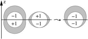
Figure 6: Gap functions for the first (left) and the second (middle) excitation branch with specified helicities of quasiparticles in the upper and the lower hemispheres. The “effective” gap relevant for the neutrino emission is shown on the right.

The asymmetry in the effective gap function translates into the asymmetry of the neutrino emission. This is due to the angular dependence of the amplitude for Urca type processes. As in the vacuum, the corresponding amplitude is proportional to $1-\cos\theta_{\nu d}$. This can be seen, for instance, from the integrand in Eq. (34). Such an angular dependence of the amplitude means that the neutrinos are emitted preferably in the direction opposite to the (almost collinear) momenta of the participating up and down quarks. In fact, this is a general property that holds also in the normal phase iwamoto . Since the effective gap function assumes smaller values for quasiparticles with $\hat{k}_{3}<0$ than with $\hat{k}_{3}>0$, there is more neutrino emission in the $+z$ direction.

One can estimate the maximum velocity of a neutron star with a quark matter core in the A phase that can be obtained by the asymmetric neutrino emission. It has been shown that this velocity is negligibly small, e.g., of the order 1 m/s, see erratum in Ref. prl . In essence, the reason for this is that the available thermal energy in the star, after matter in the stellar interior cools down to the critical temperature $T_{c}\lesssim 100$ keV of the A phase, is too small to power substantial momentum kicks. (It would be interesting to investigate, however, if additional sources of stellar heating, e.g., such as the latent heat from a first-order phase transition, could change the conclusion.)

VII Quark mass effects

In nature, quarks are not exactly massless. Therefore, it is important to address the effects that the masses have on the dispersion relations of quasiparticles, and thus on the neutrino emissivity and the specific heat of quark matter.

In order to study the massive case, we keep the color-spin structure of the gap matrix ${\cal M}_{\bf k}$ exactly as in the massless case, given in Eq. (9). Then, the inverse full quark propagator can be written as follows

$$S^{-1}(K)=\left(\begin{array}[]{cc}\left[G^{+}_{0}(K)\right]^{-1}&{\cal M}_{\bf k}\phi\\ \gamma^{0}{\cal M}_{\bf k}^{\dagger}\gamma^{0}\phi&\left[G^{-}_{0}(K)\right]^{-1}\end{array}\right)\,,$$ (61)

with $\left[G^{\pm}_{0}(K)\right]^{-1}\equiv\gamma^{\mu}K_{\mu}\pm\gamma^{0}\mu+m$, where $m$ is the quark mass. For simplicity, we omit the flavor index $f$ in this section.

We do not repeat the detailed calculations for the emissivity and the specific heat with this propagator. Instead we assume that the main modification happens due to the change of the quasiparticle dispersion relations. These relations are determined by the solution to the algebraic equation $\mbox{det}\,S^{-1}=0$, or more explicitly,

$$\mbox{det}\left[(G^{-}_{0})^{-1}(G^{+}_{0})^{-1}-\phi^{2}(G^{-}_{0})^{-1}{\cal M}_{\bf k}G^{-}_{0}\gamma^{0}{\cal M}_{\bf k}^{\dagger}\gamma^{0}\right]=0\,.$$ (62)

We find that, in all considered spin-one phases, the results for the dispersion relations are essentially the same as in the massless case, except for the replacement $k\to\sqrt{k^{2}+m^{2}}$, i.e.,

$$\epsilon_{{\bf k},r}^{2}=\left(\sqrt{k^{2}+m^{2}}-\mu\right)^{2}+\lambda_{{\bf k},r}\phi^{2}\,\,,$$ (63)

with the same $\lambda_{{\bf k},r}$’s as for $m=0$, see Table 1. This result suggests that the emissivity and the specific heat do not change qualitatively after including quark masses. This conclusion may not be so surprising because, in general, non-zero quark masses are not expected to affect much the physical properties which are dominated by quasiparticle states in the vicinity of the Fermi sphere.

In view of the above “trivial” effect of the quark masses, it is appropriate to comment on the recent study in Ref. Blaschke where it is argued that there are no ungapped modes in the CSL phase when the quarks are massive. This may look as a contradiction to our result (63), showing that all ungapped modes, $\lambda_{{\bf k},2}=0$, survive after switching on the mass. The seeming contradiction is removed, however, after noticing that a different choice of the gap matrix in the CSL phase is utilized in Ref. Blaschke . In our notation, the corresponding gap matrix would be obtained by replacing $\gamma_{\perp,j}(\hat{\mathbf{k}})$ with $\gamma_{j}$ in Eq. (9). After making such a replacement, we find that the dispersion relations of quasiparticles in Ref. Blaschke are indeed reproduced. In particular, the low-energy dispersion relations for two out of total three different quasiparticles are given by

$$\epsilon_{{\bf k},1/2}^{2} \simeq \left(\sqrt{k^{2}+m^{2}}-\mu\right)^{2}+2\,\phi^{2}\,\left(\sqrt{1+\frac{m^{2}}{8\mu^{2}}}\pm\frac{m}{2\sqrt{2}\mu}\right)^{2}\,.$$ (64)

Note that these are obtained without the limitation of the smallness of the quark mass $m$. The corresponding two energy gaps are thus

$$\phi_{1/2}=\sqrt{2}\,\phi\,\left(\sqrt{1+\frac{m^{2}}{8\mu^{2}}}\pm\frac{m}{2\sqrt{2}\mu}\right)\,.$$ (65)

The low-energy approximation, defined by $\epsilon_{{\bf k},1/2}/\mu\sim\phi/\mu\sim|\sqrt{k^{2}+m^{2}}-\mu|/\mu\ll 1$, is completely sufficient for the study of most transport and neutrino processes in spin-one color-superconducting phases.

The dispersion relation of the third quasiparticle mode can be extracted exactly,

$$\epsilon_{{\bf k},3}^{2} = \mu^{2}+k^{2}+m^{2}+\phi^{2}-2\sqrt{\mu^{2}(k^{2}+m^{2})+k^{2}\phi^{2}}$$ (66)

$$\simeq \left(\sqrt{k^{2}+m^{2}}-\mu\right)^{2}+\frac{m^{2}\phi^{2}}{\mu^{2}}\,.$$

Hence the value of the energy gap is

$$\phi_{3}=\frac{m\phi}{\sqrt{\mu^{2}+\phi^{2}}}\simeq\frac{m\phi}{\mu}\,\,.$$ (67)

For $m=0$, we recover the gaps $\phi_{1}=\phi_{2}=\sqrt{2}\,\phi$, $\phi_{3}=0$. Thus, in contrast to the massive case, both CSL gap matrices (i.e., one with $\gamma_{\perp,j}(\hat{\mathbf{k}})$ and the other with $\gamma_{j}$ in the definition of ${\cal M}_{\bf k}$) give rise to the same dispersion relations in the ultrarelativistic case. It should be studied in the future which of the two physically different CSL phases at $m\neq 0$ has the lower free energy.

VIII Conclusions

In this paper, we have computed the neutrino emissivity due to direct Urca processes (i.e., $u+e^{-}\to d+\nu$ and $d\to u+e^{-}+\bar{\nu}$), as well as the specific heat in four different spin-one color-superconducting phases of dense quark matter. Starting from the kinetic equation, we have derived a general expression for the neutrino emissivity. In the case of the normal phase of quark matter, this reduces to the well-known analytical result iwamoto . The basic ingredients in the calculation are the quasiparticle dispersion relations, containing the spin-one gap functions. We have studied in detail the effect of an isotropic gap function (CSL phase) as well as of anisotropic gap functions (planar, polar, A phases). The numerical results for the emissivity and the specific heat as functions of the ratio of the gap parameter to the temperature, $\varphi=\phi/T$, have been presented.

In all four phases, also analytical expressions have been derived in the large $\varphi$ limit (i.e., in the limit of small temperatures). In particular, in the case of an isotropic gap function (CSL phase), the well-known exponential suppression of the emissivity and the specific heat is observed. We find that anisotropic gaps give rise to different asymptotes in general. For example, the phases in which the gap has point nodes (i.e., polar and A phases) show a power-law instead of an exponential suppression at $\varphi\to\infty$. The actual form of the power-law depends on the behavior of the gap function in the vicinity of the nodes. While a linear behavior gives rise to a suppression $\sim 1/\varphi^{2}$, a quadratic behavior leads to $\sim 1/\varphi$.

We have used the results for the emissivity and the specific heat to discuss the cooling curves of spin-one color superconductors. Our simplified analysis, performed for an infinite homogeneous system, reveals several important qualitative features. Most importantly, the cooling rates of all considered spin-one color superconducting phases differ very little from that of the normal phase. The reason is that, with the choice of the gap matrix as in Eq. (9), all phases (even if the quarks are massive) have an ungapped quasiparticle mode which dominates cooling at low temperatures and, thus, makes the suppression effect due to gapped modes unobservable. Note, however, that this conclusion may change if another choice of the gap matrix, e.g., such as used in Ref. Blaschke , corresponds to the true ground state of quark matter.

In addition to the cooling rates, we have discussed an unusual property of the color-superconducting A phase, in which the neutrino emission is not symmetric under the reflection of one of the coordinate axes in position space. This is seen from the fact that the net momentum of emitted neutrinos is nonzero, pointing into a direction spontaneously picked by the order parameter. As we have argued, the asymmetry is related to the helicity properties of the quasiparticles in the A phase. A helicity order arises naturally from the structure of the gap matrix which is a straightforward generalization of the A phase in ³He (where, however, there is no helicity order).

So far, we did not find any observable consequence of the helicity order in the A phase. The simplest possibility would be realized if the asymmetric neutrino emission could result in a “neutrino rocket” mechanism for stars prl . The estimated effect on the stellar velocity appears to be extremely small, however. The search for other observable signatures, e.g., dealing with the timing of pulsars, may reveal other possibilities. We could also imagine that observable signatures of the helicity-type order might be observed in completely different systems in atomic or condensed matter physics (e.g., trapped gases of cold fermionic atoms, or high-$T_{c}$ superconductors) if they happen to have a similar structure of the order parameter, see for example Ref. helicity-cond-mat . A systematic study of such a possibility is outside the scope of this paper, however.

Appendix A Matsubara sum

In the calculation of the polarization tensor $\Pi_{R}^{\lambda\sigma}(Q)$ in Sec. II we use the following Matsubara sum,

$$T\sum_{k_{0}}\frac{(k_{0}+\xi_{1})(k_{0}+q_{0}+\xi_{2})}{(k_{0}^{2}-\epsilon_{1}^{2})[(k_{0}+q_{0})^{2}-\epsilon_{2}^{2}]} = \frac{1}{4\epsilon_{1}\epsilon_{2}}\left\{\left[\frac{(\epsilon_{1}-\xi_{1})(\epsilon_{2}+\xi_{2})}{q_{0}-\epsilon_{1}-\epsilon_{2}}-\frac{(\epsilon_{1}+\xi_{1})(\epsilon_{2}-\xi_{2})}{q_{0}+\epsilon_{1}+\epsilon_{2}}\right]\left[1-n_{F}(\epsilon_{1})-n_{F}(\epsilon_{2})\right]\right.$$ (68)

$$\left.+\;\left[\frac{(\epsilon_{1}+\xi_{1})(\epsilon_{2}+\xi_{2})}{q_{0}+\epsilon_{1}-\epsilon_{2}}-\frac{(\epsilon_{1}-\xi_{1})(\epsilon_{2}-\xi_{2})}{q_{0}-\epsilon_{1}+\epsilon_{2}}\right]\left[n_{F}(\epsilon_{1})-n_{F}(\epsilon_{2})\right]\right\}\,\,,$$

where $k_{0}$ ($q_{0}$) is the fermionic (bosonic) energy and $\xi_{1},\xi_{2},\epsilon_{1},\epsilon_{2}$ are real numbers ($\epsilon_{1},\epsilon_{2}>0$). With

$$1-n_{F}(\epsilon_{1})-n_{F}(\epsilon_{2})=\frac{n_{F}(\epsilon_{1})\,n_{F}(\epsilon_{2})}{n_{B}(\epsilon_{1}+\epsilon_{2})}=-\frac{n_{F}(-\epsilon_{1})\,n_{F}(-\epsilon_{2})}{n_{B}(-\epsilon_{1}-\epsilon_{2})}$$ (69)

and

$$n_{F}(\epsilon_{1})-n_{F}(\epsilon_{2})=\frac{n_{F}(-\epsilon_{1})\,n_{F}(\epsilon_{2})}{n_{B}(-\epsilon_{1}+\epsilon_{2})}=-\frac{n_{F}(\epsilon_{1})\,n_{F}(-\epsilon_{2})}{n_{B}(\epsilon_{1}-\epsilon_{2})}$$ (70)

we can write the result in the following compact form,

$$T\sum_{k_{0}}\frac{(k_{0}+\xi_{1})(k_{0}+q_{0}+\xi_{2})}{(k_{0}^{2}-\epsilon_{1}^{2})[(k_{0}+q_{0})^{2}-\epsilon_{2}^{2}]}=-\frac{1}{4\epsilon_{1}\epsilon_{2}}\sum_{e_{1},e_{2}=\pm}\frac{(\epsilon_{1}-e_{1}\xi_{1})\,(\epsilon_{2}-e_{2}\xi_{2})}{q_{0}-e_{1}\epsilon_{1}+e_{2}\epsilon_{2}}\,\frac{n_{F}(-e_{1}\epsilon_{1})\,n_{F}(e_{2}\epsilon_{2})}{n_{B}(-e_{1}\epsilon_{1}+e_{2}\epsilon_{2})}\,\,.$$ (71)

This formula is applied to Eq. (21).

Appendix B Color and Dirac traces

In this appendix, we compute the color and Dirac traces of the tensor ${\cal T}_{rs,+}^{\lambda\sigma}(\hat{\mathbf{k}},\hat{\mathbf{p}})$, see Eq. (22), in the polar, planar, A, and CSL phases. Moreover, we contract this tensor with the tensor $L^{\lambda\sigma}({\bf p}_{e},{\bf p})$, see Eq. (5), to obtain the functions $\omega_{rs}(\hat{\mathbf{k}},\hat{\mathbf{p}})$, see Eq. (28). In this appendix, for the sake of clarity, we shall add the subscripts $c$ or $D$ at the symbol “Tr” to indicate whether the trace is taken over color or Dirac space. In the calculation, we encounter the following expressions,

$$L^{00}({\bf p}_{e},{\bf p}_{\nu}) = 8\,(p_{e}p_{\nu}+{\bf p}_{e}\cdot{\bf p_{\nu}})\,\,,$$ (72a)

$$L^{0i}({\bf p}_{e},{\bf p}_{\nu}) = 8\,[p_{e}p_{\nu}^{i}+p_{e}^{i}p_{\nu}+i\,({\bf p}_{e}\times{\bf p_{\nu}})_{i}]\,\,,$$ (72b)

$$L^{i0}({\bf p}_{e},{\bf p}_{\nu}) = 8\,[p_{e}p_{\nu}^{i}+p_{e}^{i}p_{\nu}-i\,({\bf p}_{e}\times{\bf p_{\nu}})_{i}]\,\,,$$ (72c)

$$L^{ij}({\bf p}_{e},{\bf p}_{\nu}) = 8\,[\delta^{ij}(p_{e}p_{\nu}-{\bf p}_{e}\cdot{\bf p_{\nu}})+p_{e}^{i}p_{\nu}^{j}+p_{e}^{j}p_{\nu}^{i}-i\,\epsilon^{ij\ell}\,(p_{e}p_{\nu}^{\ell}-p_{e}^{\ell}p_{\nu})]\,\,,$$ (72d)

where $i,j=1,2,3$, and

$${\cal T}^{00}(\hat{\mathbf{k}},\hat{\mathbf{p}}) = 2\,(1+\hat{\mathbf{k}}\cdot\hat{\mathbf{p}})\,\,,$$ (73a)

$${\cal T}^{0i}(\hat{\mathbf{k}},\hat{\mathbf{p}}) = 2\,[\hat{k}^{i}+\hat{p}^{i}+i\,(\hat{\mathbf{k}}\times\hat{\mathbf{p}})]\,\,,$$ (73b)

$${\cal T}^{i0}(\hat{\mathbf{k}},\hat{\mathbf{p}}) = 2\,[\hat{k}^{i}+\hat{p}^{i}-i\,(\hat{\mathbf{k}}\times\hat{\mathbf{p}})]\,\,,$$ (73c)

$${\cal T}^{ij}(\hat{\mathbf{k}},\hat{\mathbf{p}}) = 2\,[\delta^{ij}(1-\hat{\mathbf{k}}\cdot\hat{\mathbf{p}})+\hat{k}^{i}\hat{p}^{j}+\hat{k}^{j}\hat{p}^{i}+i\,\epsilon^{ij\ell}\,(\hat{k}^{\ell}-\hat{p}^{\ell})]\,\,,$$ (73d)

where we abbreviated

$${\cal T}^{\lambda\sigma}(\hat{\mathbf{k}},\hat{\mathbf{p}})\equiv{\rm Tr}_{D}\left[\gamma^{\lambda}(1-\gamma^{5})\,\gamma^{0}\,\,\Lambda_{\bf k}^{-}\,\gamma^{\sigma}(1-\gamma^{5})\,\gamma^{0}\,\Lambda_{\bf p}^{-}\right]\,\,.$$ (74)

Using the above results, we calculate the Lorentz contraction

$$L_{\lambda\sigma}({\bf p}_{e},{\bf p}_{\nu})\,{\cal T}^{\lambda\sigma}(\hat{\mathbf{k}},\hat{\mathbf{p}})=64\,(p_{e}-{\bf p}_{e}\cdot\hat{\mathbf{k}})\,(p_{\nu}-{\bf p}_{\nu}\cdot\hat{\mathbf{p}})\,\,.$$ (75)

This is a generic result which we shall use in the following subsections to compute the more complicated contractions for the spin-one phases.

B.1 Polar phase

The polar phase is particularly simple, since the projection operators ${\cal P}_{{\bf k},r}^{+}$ do not depend on the quark momentum ${\bf k}$. With

$${\cal P}_{{\bf k},1}^{+}=J_{3}^{2}\,\,,\qquad{\cal P}_{{\bf k},2}^{+}=1-J_{3}^{2}\,\,,$$ (76)

we immediately find after performing the color trace

$$\omega_{11}(\hat{\mathbf{k}},\hat{\mathbf{p}})=2\,\,,\qquad\omega_{22}(\hat{\mathbf{k}},\hat{\mathbf{p}})=1\,\,,\qquad\omega_{12}(\hat{\mathbf{k}},\hat{\mathbf{p}})=\omega_{21}(\hat{\mathbf{k}},\hat{\mathbf{p}})=0\,\,.$$ (77)

B.2 Planar phase

In the planar phase, we have

$${\cal P}_{{\bf k},1}^{+}=\frac{1}{1+\hat{k}^{2}_{3}}\,\left[J_{1}^{2}\,(1-\hat{k}_{1}^{2})+J_{2}^{2}\,(1-\hat{k}_{2}^{2})-\{J_{1},J_{2}\}\,\hat{k}_{1}\hat{k}_{2}+J_{3}\,\hat{k}_{3}\gamma^{0}\gamma^{5}\bm{\gamma}\cdot\hat{\mathbf{k}}\right]\,\,,\qquad{\cal P}_{{\bf k},2}^{+}=1-{\cal P}_{{\bf k},1}^{+}\,\,,$$ (78)

where $\{J_{1},J_{2}\}$ denotes the anticommutator of $J_{1}$ and $J_{2}$. In order to perform the color traces, we use $J_{i}^{4}=J_{i}^{2}$ $(i=1,2)$ and

$${\rm Tr}_{c}[J_{i}^{2}]=2\quad(i=1,2,3)\,\,,\qquad{\rm Tr}_{c}[J_{1}^{2}J_{2}^{2}]=1\,\,,\qquad{\rm Tr}_{c}[\{J_{1},J_{2}\}^{2}]=2\,\,,$$

$${\rm Tr}_{c}[J_{i}^{2}J_{3}]={\rm Tr}_{c}[J_{i}^{2}\{J_{1},J_{2}\}]=0\quad(i=1,2)\,\,.$$ (79)

The only apparently additional Dirac trace which occurs in this phase is in fact identical to the above one,

$${\rm Tr}_{D}\left[\gamma^{\lambda}(1-\gamma^{5})\,\gamma^{5}\,\bm{\gamma}\cdot\hat{\mathbf{k}}\,\Lambda_{\bf k}^{-}\,\gamma^{\sigma}(1-\gamma^{5})\,\gamma^{5}\,\bm{\gamma}\cdot\hat{\mathbf{p}}\,\Lambda_{\bf p}^{-}\right]={\cal T}^{\lambda\sigma}(\hat{\mathbf{k}},\hat{\mathbf{p}})\,\,.$$ (80)

Consequently, with Eq. (75) we find

$$\omega_{11}(\hat{\mathbf{k}},\hat{\mathbf{p}})=\frac{1}{2}\,[3+\eta(\hat{\mathbf{k}},\hat{\mathbf{p}})]\,\,,\qquad\omega_{22}(\hat{\mathbf{k}},\hat{\mathbf{p}})=\frac{1}{2}\,[1+\eta(\hat{\mathbf{k}},\hat{\mathbf{p}})]\,\,,\qquad\omega_{12}(\hat{\mathbf{k}},\hat{\mathbf{p}})=\omega_{21}(\hat{\mathbf{k}},\hat{\mathbf{p}})=\frac{1}{2}\,[1-\eta(\hat{\mathbf{k}},\hat{\mathbf{p}})]\,\,,$$ (81)

where

$$\eta(\hat{\mathbf{k}},\hat{\mathbf{p}})\equiv\frac{4\hat{k}_{3}\hat{p}_{3}+(\hat{k}_{1}\hat{p}_{1}+\hat{k}_{2}\hat{p}_{2})^{2}-(\hat{k}_{1}\hat{p}_{2}-\hat{k}_{2}\hat{p}_{1})^{2}}{(1+\hat{k}_{3}^{2})(1+\hat{p}_{3}^{2})}\,\,.$$ (82)

B.3 A phase

In this case, there are three different quasiparticle branches. Hence, we have three projection operators,

$${\cal P}_{{\bf k},1}^{+}=\frac{1}{2}J_{3}^{2}\left[1+{\rm sgn}(\hat{k}_{3})\,\gamma^{0}\gamma^{5}\bm{\gamma}\cdot\hat{\mathbf{k}}\right]\,\,,\qquad{\cal P}_{{\bf k},2}^{+}=\frac{1}{2}J_{3}^{2}\left[1-{\rm sgn}(\hat{k}_{3})\,\gamma^{0}\gamma^{5}\bm{\gamma}\cdot\hat{\mathbf{k}}\right]\,\,,\qquad{\cal P}_{{\bf k},3}^{+}=1-J_{3}^{2}\,\,.$$ (83)

Again, all Dirac traces can be reduced to the previous one, because of Eq. (80) and

$${\rm Tr}_{D}\left[\gamma^{\lambda}(1-\gamma^{5})\,\gamma^{5}\,\bm{\gamma}\cdot\hat{\mathbf{k}}\,\Lambda_{\bf k}^{-}\,\gamma^{\sigma}(1-\gamma^{5})\,\gamma^{0}\,\Lambda_{\bf p}^{-}\right]$$

$$={\rm Tr}_{D}\left[\gamma^{\lambda}(1-\gamma^{5})\,\gamma^{0}\,\Lambda_{\bf k}^{-}\,\gamma^{\sigma}(1-\gamma^{5})\,\gamma^{5}\,\bm{\gamma}\cdot\hat{\mathbf{p}}\,\Lambda_{\bf p}^{-}\right]={\cal T}^{\lambda\sigma}(\hat{\mathbf{k}},\hat{\mathbf{p}})\,\,.$$ (84)

We thus find immediately, again using Eq. (75),

$$\omega_{11}(\hat{\mathbf{k}},\hat{\mathbf{p}}) = \frac{1}{2}[1+{\rm sgn}(\hat{k}_{3})][1+{\rm sgn}(\hat{p}_{3})]\,\,,\qquad\omega_{22}(\hat{\mathbf{k}},\hat{\mathbf{p}})=\frac{1}{2}[1-{\rm sgn}(\hat{k}_{3})][1-{\rm sgn}(\hat{p}_{3})]\,\,,$$ (85)

$$\omega_{12}(\hat{\mathbf{k}},\hat{\mathbf{p}}) = \frac{1}{2}[1+{\rm sgn}(\hat{k}_{3})][1-{\rm sgn}(\hat{p}_{3})]\,\,,\qquad\omega_{21}(\hat{\mathbf{k}},\hat{\mathbf{p}})=\frac{1}{2}[1-{\rm sgn}(\hat{k}_{3})][1+{\rm sgn}(\hat{p}_{3})]\,\,,$$ (86)

$$\omega_{33}(\hat{\mathbf{k}},\hat{\mathbf{p}}) = 1\,\,,\qquad\omega_{13}(\hat{\mathbf{k}},\hat{\mathbf{p}})=\omega_{31}(\hat{\mathbf{k}},\hat{\mathbf{p}})=\omega_{23}(\hat{\mathbf{k}},\hat{\mathbf{p}})=\omega_{32}(\hat{\mathbf{k}},\hat{\mathbf{p}})=0\,\,.$$ (87)

All vanishing functions $\omega_{rs}(\hat{\mathbf{k}},\hat{\mathbf{p}})$ are zero because of a vanishing color trace. This is exactly as in the polar phase where also all functions $\omega_{rs}(\hat{\mathbf{k}},\hat{\mathbf{p}})$, that include one gapped and one ungapped branch, vanish.

B.4 CSL phase

In the CSL phase,

$${\cal P}_{{\bf k},1}^{+}=-\frac{1}{2}\left[{\bf J}\cdot\bm{\gamma}_{\perp}(\hat{\mathbf{k}})\right]^{2}\,\,,\qquad{\cal P}_{{\bf k},2}^{+}=1+\frac{1}{2}\left[{\bf J}\cdot\bm{\gamma}_{\perp}(\hat{\mathbf{k}})\right]^{2}\,\,.$$ (88)

It is convenient to write these projectors with the help of color indices $a,b=1,2,3$,

$$\left({\cal P}_{{\bf k},1}^{+}\right)_{ab}=\delta_{ab}+\frac{1}{2}\gamma_{\perp,b}(\hat{\mathbf{k}})\gamma_{\perp,a}(\hat{\mathbf{k}})\,\,,\qquad\left({\cal P}_{{\bf k},2}^{+}\right)_{ab}=-\frac{1}{2}\gamma_{\perp,b}(\hat{\mathbf{k}})\gamma_{\perp,a}(\hat{\mathbf{k}})\,\,.$$ (89)

Using these expressions, we compute the color and Dirac traces. The only additional nontrivial trace that occurs can again be expressed in terms of the previous one,

$$\sum_{a,b=1}^{3}\,{\rm Tr}_{D}\left[\gamma^{\lambda}(1-\gamma^{5})\,\gamma^{0}\,\gamma_{\perp,a}(\hat{\mathbf{k}})\gamma_{\perp,b}(\hat{\mathbf{k}})\,\Lambda_{\bf k}^{-}\,\gamma^{\sigma}(1-\gamma^{5})\,\gamma^{0}\,\gamma_{\perp,b}(\hat{\mathbf{p}})\gamma_{\perp,a}(\hat{\mathbf{p}})\,\Lambda_{\bf p}^{-}\right]=(1+\hat{\mathbf{k}}\cdot\hat{\mathbf{p}})^{2}\,{\cal T}^{\lambda\sigma}(\hat{\mathbf{k}},\hat{\mathbf{p}})\,\,.$$ (90)

Then, with Eq. (75) we find

$$\omega_{11}(\hat{\mathbf{k}},\hat{\mathbf{p}}) = 1+\frac{1}{4}(1+\hat{\mathbf{k}}\cdot\hat{\mathbf{p}})^{2}\,\,,\qquad\omega_{22}(\hat{\mathbf{k}},\hat{\mathbf{p}})=\frac{1}{4}(1+\hat{\mathbf{k}}\cdot\hat{\mathbf{p}})^{2}\,\,,$$

$$\omega_{12}(\hat{\mathbf{k}},\hat{\mathbf{p}}) = \omega_{21}(\hat{\mathbf{k}},\hat{\mathbf{p}})=1-\frac{1}{4}(1+\hat{\mathbf{k}}\cdot\hat{\mathbf{p}})^{2}\,\,.$$ (91)

Note that we have also used the following identity,

$$\sum_{a=1}^{3}\left[\gamma_{\perp,a}(\hat{\mathbf{k}})\right]^{2}=-2\,\,.$$ (92)

Appendix C Angular Integrals

Here we compute the integral

$$I({\bf p}_{\nu})\equiv\int d\Omega_{\bf p}\int d\Omega_{\bf k}(1-\cos\theta_{\nu d})\,\delta(\cos\theta_{0}-\cos\theta_{ud})\,F(\hat{\mathbf{k}},\hat{\mathbf{p}})\,\,.$$ (93)

The result shall be applied to Eq. (34). Thus, the function $F(\hat{\mathbf{k}},\hat{\mathbf{p}})$ stands for $F^{rs}_{\varphi_{u}\varphi_{d}}(\hat{\mathbf{k}},\hat{\mathbf{p}},v)$, defined in Eq. (35), i.e., for notational convenience we omit all indices since only the dependence on $\hat{\mathbf{k}}$ and $\hat{\mathbf{p}}$ is of relevance. For the definition of $\cos\theta_{0}$ see text below Eqs. (31).

There is a fixed direction in position space, defined by the order parameter. We choose our frame such that the $z$-axis points into this direction. Moreover, for the $d\Omega_{\bf k}$ integration, we may choose the frame such that the three-momentum of the $d$ quark, ${\bf p}$, lies in the $xz$-plane. Then, we can write the unit vectors of the momenta of $u$ quark, $d$ quark, and neutrino as

$$\hat{\mathbf{k}}=\left(\begin{array}[]{c}\sin\theta_{u}\cos\varphi_{u}\\ \sin\theta_{u}\sin\varphi_{u}\\ \cos\theta_{u}\end{array}\right)\,\,,\qquad\hat{\mathbf{p}}=\left(\begin{array}[]{c}\sin\theta_{d}\\ 0\\ \cos\theta_{d}\end{array}\right)\,\,,\qquad\hat{\mathbf{p}}_{\nu}=\left(\begin{array}[]{c}\sin\theta_{\nu}\cos\varphi_{\nu}\\ \sin\theta_{\nu}\sin\varphi_{\nu}\\ \cos\theta_{\nu}\end{array}\right)\,\,,$$ (94)

respectively, and $\cos\theta_{ud}=\hat{\mathbf{k}}\cdot\hat{\mathbf{p}}$, $\cos\theta_{\nu d}=\hat{\mathbf{p}}_{\nu}\cdot\hat{\mathbf{p}}$. (In this appendix, no confusion of the angle $\varphi_{u}$ with the ratio $\varphi_{u}=\phi_{u}/T$ is possible.) In the chosen frame, the most general angular dependence of the function $F$, which applies for all phases we consider, is

$$F(\hat{\mathbf{k}},\hat{\mathbf{p}})=F(\cos\theta_{u},\cos\theta_{d},\sin\theta_{u}\sin\theta_{d},\cos\varphi_{u})\,\,,$$ (95)

The angular dependencies enter this function through the eigenvalues $\lambda_{{\bf k},r}$, $\lambda_{{\bf p},s}$ and the functions $\omega_{rs}(\hat{\mathbf{k}},\hat{\mathbf{p}})$. In the CSL phase, the eigenvalues are constant. However, the functions $\omega_{rs}$ depend on the scalar product $\hat{\mathbf{k}}\cdot\hat{\mathbf{p}}$, wherefore the arguments $\sin\theta_{u}\sin\theta_{d}$ and $\cos\varphi_{u}$ enter the function $F$. In all other phases, $\lambda_{{\bf k},r}$ and $\lambda_{{\bf p},s}$ are angular dependent. They depend only on $\cos\theta_{u}$ and $\cos\theta_{d}$, respectively. The functions $\omega_{rs}$ are constant in the polar phase, whereas they depend on $\cos\theta_{u}$ and $\cos\theta_{d}$ in the A phase. In the planar phase, the angular dependence of the functions $\omega_{rs}$ seems complicated, see Eqs. (81) and (82). However, with $\hat{p}_{2}=0$, the only additional argument is $\cos\varphi_{u}$.

Let us abbreviate $\xi_{i}\equiv\cos\theta_{i}$ ($i=u,d,0$). Then,

$$I({\bf p}_{\nu}) = \int d\Omega_{\bf p}\,(1-\cos\theta_{\nu d})\,\int_{0}^{2\pi}d\varphi_{u}\int_{-1}^{1}d\xi_{u}\,\delta\left(\xi_{0}-\xi_{u}\xi_{d}-\sqrt{(1-\xi_{u}^{2})(1-\xi_{d}^{2})}\,\cos\varphi_{u}\right)$$ (96)

$$\times\;F(\xi_{u},\xi_{d},\sqrt{(1-\xi_{u}^{2})(1-\xi_{d}^{2})},\cos\varphi_{u})\,\,.$$

Due to the $\delta$-function, the integral is only nonzero if

$$\left|\frac{\xi_{0}-\xi_{u}\xi_{d}}{\sqrt{(1-\xi_{u}^{2})(1-\xi_{d}^{2})}}\right|<1\,\,,$$ (97)

or, equivalently, if $\xi_{u}^{-}<\xi_{u}<\xi_{u}^{+}$, where

$$\xi_{u}^{\pm}\equiv\xi_{0}\xi_{d}\pm\sqrt{(1-\xi_{0}^{2})(1-\xi_{d}^{2})}\,\,.$$ (98)

Consequently,

$$I({\bf p}_{\nu}) = 2\,\int d\Omega_{\bf p}\,(1-\cos\theta_{\nu d})\,\int_{\xi_{u}^{-}}^{\xi_{u}^{+}}d\xi_{u}\,\frac{F\left(\xi_{u},\xi_{d},\sqrt{(1-\xi_{u}^{2})(1-\xi_{d}^{2})},\frac{\xi_{0}-\xi_{u}\xi_{d}}{\sqrt{(1-\xi_{u}^{2})(1-\xi_{d}^{2})}}\right)}{\sqrt{(1-\xi_{u}^{2})(1-\xi_{d}^{2})-(\xi_{0}-\xi_{u}\xi_{d})^{2}}}\,\,.$$ (99)

In order to perform the $\xi_{u}$ integral explicitly, we introduce the new variable $\xi_{u}^{\prime}=(\xi_{u}-\xi_{0}\xi_{d})/\sqrt{(1-\xi_{0}^{2})(1-\xi_{d}^{2})}$ with the integration range from $-1$ to $1$. In terms of the new variable, the integrand becomes a non-singular function of $\xi_{0}$ when $\xi_{0}\to 1$. Because of the kinematics of the Urca processes, see text after Eqs. (29), the actual value of $\xi_{0}\simeq 1-\kappa\mu_{e}^{2}/(\mu_{u}\mu_{d})$ is very close to 1. Therefore, to leading order, we may set $\xi_{0}=1$. Then, the integral over $\xi_{u}^{\prime}$ can be performed analytically, and we arrive at

$$I({\bf p}_{\nu})\simeq 2\pi\int d\Omega_{\bf p}\,(1-\cos\theta_{\nu d})\,F(\xi_{d},\xi_{d},1-\xi_{d}^{2},1)\,\,.$$ (100)

The arguments in the function $F$ show that the leading result is obtained from $\hat{\mathbf{k}}\simeq\hat{\mathbf{p}}$. Applying this approximation to the results of the previous appendix, we see that the functions $\omega_{rs}$ become constant in the case of the planar and CSL phase. (Note, in particular, that $\eta(\hat{\mathbf{k}},\hat{\mathbf{k}})=1$ in the planar phase.)

In order to perform the $d\Omega_{\bf p}$ integration, we have to reinstall the second component of the $d$ quark momentum, $\hat{p}_{2}=\sin\theta_{d}\sin\varphi_{d}$, in the term $\cos\theta_{\nu d}$. We may perform the integral over $\varphi_{d}$ and obtain

$$I({\bf p}_{\nu})\simeq 4\pi^{2}\int_{-1}^{1}d\xi(1-\xi\cos\theta_{\nu})\,F(\xi,\xi,1-\xi^{2},1)\,\,.$$ (101)

Appendix D Emissivity at low temperature

In this appendix, we compute the $\varphi$ dependence of the function $G(\varphi,\varphi)$, cf. definition (41), for $\varphi\to\infty$. This corresponds to the behavior of the neutrino emissivity of the gapped modes for small temperatures. For the phases in which the gap function has no nodes (CSL and planar phases), it is useful to compute the asymptotic behavior of the following integral separately,

$$I(\varphi,\varphi) \equiv \sum_{e_{1},e_{2}=\pm}\int_{0}^{\infty}dv\,v^{3}\,\int_{0}^{\infty}dx\,\int_{0}^{\infty}dy\,\left(e^{-e_{1}\sqrt{y^{2}+\varphi^{2}}}+1\right)^{-1}\,\left(e^{e_{2}\sqrt{x^{2}+\varphi^{2}}}+1\right)^{-1}$$ (102)

$$\times\;\left(e^{v+e_{1}\sqrt{y^{2}+\varphi^{2}}-e_{2}\sqrt{x^{2}+\varphi^{2}}}+1\right)^{-1}\,\,.$$

After performing the summation over $e_{1}$ and $e_{2}$ explicitly and taking into account that $\exp(\sqrt{x^{2}+\varphi^{2}})\gg 1$ and $\exp(\sqrt{y^{2}+\varphi^{2}})\gg 1$, we arrive at the following expression,

$$I(\varphi,\varphi) \simeq \int_{0}^{\infty}dv\,v^{3}\,\int_{0}^{\infty}dx\,\int_{0}^{\infty}dy\,\Bigg{(}\frac{1}{e^{\sqrt{x^{2}+\varphi^{2}}}+e^{v+\sqrt{y^{2}+\varphi^{2}}}}+\frac{1}{e^{v+\sqrt{x^{2}+\varphi^{2}}}+e^{\sqrt{y^{2}+\varphi^{2}}}}$$ (103)

$$+\frac{1}{e^{v}+e^{\sqrt{x^{2}+\varphi^{2}}+\sqrt{y^{2}+\varphi^{2}}}}+\frac{1}{e^{v+\sqrt{x^{2}+\varphi^{2}}+\sqrt{y^{2}+\varphi^{2}}}}\Bigg{)}\,.$$

Both the third and fourth terms in the integrand yield contributions of the order of $\exp(-2\varphi)$. For the third term we obtain

$$\int_{0}^{\infty}dv\,v^{3}\,\int_{0}^{\infty}dx\,\int_{0}^{\infty}dy\,\frac{1}{e^{v}+e^{\sqrt{x^{2}+\varphi^{2}}+\sqrt{y^{2}+\varphi^{2}}}} = -6\int_{0}^{\infty}dx\,\int_{0}^{\infty}dy\,e^{-\sqrt{x^{2}+\varphi^{2}}-\sqrt{y^{2}+\varphi^{2}}}$$ (104)

$$\times\,\mbox{Li}_{4}(-e^{\sqrt{x^{2}+\varphi^{2}}+\sqrt{y^{2}+\varphi^{2}}})$$

$$\simeq 2\pi\,\varphi^{5}\,e^{-2\varphi}\,\,,$$

where we used the asymptotic behavior of the polylogarithm $\mbox{Li}_{4}(-e^{z})\simeq-\frac{1}{24}z^{4}$ for $z\to\infty$. The fourth term yields

$$\int_{0}^{\infty}dv\,v^{3}\,\int_{0}^{\infty}dx\,\int_{0}^{\infty}dy\,\frac{1}{e^{v+\sqrt{x^{2}+\varphi^{2}}+\sqrt{y^{2}+\varphi^{2}}}}\simeq 3\pi\,\varphi\,\exp(-2\varphi)$$ (105)

We neglect both contributions (104) and (105) to the integral $I(\varphi,\varphi)$ since they are suppressed stronger than the first two terms terms in Eq. (103). The latter yield contributions of the order of $\exp(-\varphi)$,

$$I(\varphi,\varphi) \simeq 2\,\int_{0}^{\infty}dv\,v^{3}\,\int_{0}^{\infty}dx\,\int_{0}^{\infty}dy\,\frac{e^{-\varphi}}{e^{x^{2}/(2\varphi)}+e^{v+y^{2}/(2\varphi)}}$$ (106)

$$= 4\varphi e^{-\varphi}\int_{0}^{\infty}dv\,v^{3}\,\int_{0}^{\infty}dx\,\int_{0}^{\infty}dy\,\frac{1}{e^{x^{2}}+e^{v+y^{2}}}$$

$$\simeq 42.55\,\varphi\,e^{-\varphi}\,,$$

where the overall number is obtained by performing the numerical integration.

D.1 CSL phase

Using Eqs. (37), (41a), (106), and $\lambda_{\xi,1}=2$ (see Table 2) we immediately conclude

$$G(\varphi,\varphi) = \frac{5040}{457\,\pi^{6}}\,I(\sqrt{2}\varphi,\sqrt{2}\varphi)$$ (107)

$$\simeq 0.69\,\varphi\,e^{-\sqrt{2}\varphi}\,\,.$$

D.2 Planar phase

For the planar phase, we may also use Eq. (106) because the gap function has no nodes around the Fermi sphere. However, the result contains an additional angular integration. Using Eqs. (37), (41a), and $\lambda_{\xi,1}=1+\xi^{2}$, we derive

$$G(\varphi,\varphi)=\frac{2520}{457\,\pi^{6}}\,\int_{-1}^{1}d\xi\,I(\sqrt{1+\xi^{2}}\,\varphi,\sqrt{1+\xi^{2}}\,\varphi)\,.$$ (108)

Approximating the angular integral as

$$\int_{-1}^{1}d\xi\,\sqrt{1+\xi^{2}}\,e^{-\sqrt{1+\xi^{2}}\varphi}\simeq\int_{-\infty}^{\infty}d\xi\,e^{-(1+\xi^{2}/2)\varphi}=\sqrt{2\pi}\,\frac{e^{-\varphi}}{\sqrt{\varphi}}\,\,,$$ (109)

we obtain

$$G(\varphi,\varphi)\simeq 0.61\,\sqrt{\varphi}\,e^{-\varphi}\,\,.$$ (110)

D.3 Polar phase

In the polar phase, the low temperature behavior of the neutrino emissivity is dominated by the regions around the nodes of the gap function. Since $\lambda_{{\bf k},1}=\sin^{2}\theta_{\bf k}$, the dominant contribution comes from the vicinities of the north and south pole of the Fermi sphere. The gap behaves linear around these points, $\sqrt{\lambda_{{\bf k},1}}\simeq\theta_{\bf k}$. To obtain the leading order result in $\varphi$, we integrate over the region where the quasiparticle energy is less than or of the order of the scale set by the temperature, i.e., $\sqrt{\lambda_{{\bf k},1}}\,\phi\lesssim\pi\,T$, or, equivalently, $\theta_{\bf k}\lesssim\pi/\varphi$ (and analogously for the south pole of the Fermi sphere). Consequently, we may use Eq. (41a), set $\varphi_{u}=\varphi_{d}=0$ and integrate over the appropriate angular regions. Then, upon using $\omega_{11}(\xi)=2$ (see Table 2) and the integral (39) we obtain

$$G(\varphi,\varphi)\simeq\int_{0}^{\pi/\varphi}d\theta_{\bf k}\,\theta_{\bf k}=\frac{\pi^{2}}{2\varphi^{2}}\simeq\frac{4.93}{\varphi^{2}}\,\,.$$ (111)

D.4 A phase

As in the polar phase, the dominant contribution comes from the nodes of the gap function. Therefore, we can neglect the term corresponding to the first (fully gapped) branch in Eq. (41b). We keep the term that corresponds to the gap function given by $\lambda_{{\bf k},2}=(1-|\cos\theta_{\bf k}|)^{2}$. In contrast to the polar phase, the gap function behaves quadratically in the angular directions in the vicinity of the nodes, $\sqrt{\lambda_{{\bf k},2}}\simeq\theta_{\bf k}^{2}/2$. Therefore, in order to be consistent with the estimate in the polar phase, we restrict the integral to the regions $0<\theta_{\bf k}<\sqrt{2\pi/\varphi}$ and $\pi-\sqrt{2\pi/\varphi}<\theta_{\bf k}<\pi$. With $\omega_{22}(\xi)=1-{\rm sgn}(\xi)$ we obtain

$$G(\varphi,\varphi)\simeq\frac{1}{2}\int_{\pi-\sqrt{2\pi/\varphi}}^{\pi}d\theta_{\bf k}\,(\pi-\theta_{\bf k})=\frac{\pi}{2\varphi}\simeq\frac{1.57}{\varphi}\,\,.$$ (112)

Note that due to the factor $\omega_{22}(\xi)$, in fact only one of the nodes, $\theta_{\bf k}=\pi$, yields a nonzero contribution. The physical reason for this is explained in detail in Sec. VI.

Appendix E Specific heat at low temperature

Here we compute the behavior of the function $K(\varphi)$, cf. definition (47), for $\varphi\to\infty$. Physically, this corresponds to the behavior of the specific heat of the gapped modes for small temperatures. From Eqs. (47) we conclude that for large $\varphi$ and hence $\varphi^{2}\gg\phi_{0}^{2}/T_{c}^{2}$

$$K(\varphi) \simeq \frac{3}{2\pi^{2}}\int_{0}^{\infty}dx\,\int_{-1}^{1}d\xi\,(x^{2}+\lambda_{\xi,1}\,\varphi^{2})\,\frac{1}{1+\cosh\left(\sqrt{x^{2}+\lambda_{\xi,1}\varphi^{2}}\right)}\qquad\mbox{(CSL, planar, polar)}\,\,,$$ (113a)

$$K(\varphi) \simeq \frac{3}{4\pi^{2}}\sum_{r=1}^{2}\int_{0}^{\infty}dx\,x^{2}\int_{-1}^{1}d\xi\,(x^{2}+\lambda_{\xi,r}\varphi^{2})\,\frac{1}{1+\cosh\left(\sqrt{x^{2}+\lambda_{\xi,1}\varphi^{2}}\right)}\qquad(A)\,\,.$$ (113b)

E.1 CSL phase

In the CSL phase, $\lambda_{\xi,1}=2$, thus the angular integration $d\xi$ is trivial. Moreover, we may approximate

$$\frac{1}{1+\cosh\left(\sqrt{x^{2}+\lambda_{\xi,1}\varphi^{2}}\right)}\simeq 2\,e^{-\sqrt{x^{2}+2\varphi^{2}}}\simeq 2\,e^{-\sqrt{2}\,\varphi-\frac{x^{2}}{2\sqrt{2}\varphi}}\,\,.$$ (114)

Consequently,

$$K(\varphi)\simeq\frac{6}{\pi^{2}}\int_{0}^{\infty}dx\,(x^{2}+2\varphi^{2})\,e^{-\sqrt{2}\,\varphi-\frac{x^{2}}{2\sqrt{2}\varphi}}\simeq\frac{3\sqrt{2}}{\pi^{3/2}}\,(\sqrt{2}\,\varphi)^{5/2}\,e^{-\sqrt{2}\,\varphi}\simeq 1.81\,\varphi^{5/2}\,e^{-\sqrt{2}}\,\,.$$ (115)

E.2 Planar phase

As in the CSL phase, the gap has no nodes in the planar phase. Therefore, a similar approximation can be used,

$$K(\varphi) \simeq \frac{3}{\pi^{2}}\int_{-1}^{1}d\xi\,e^{-\sqrt{1+\xi^{2}}\,\varphi}\,\int_{0}^{\infty}dx\,\left[x^{2}+(1+\xi^{2})\,\varphi^{2}\right]\,e^{-\frac{x^{2}}{2\sqrt{1+\xi^{2}}\,\varphi}}$$ (116)

$$\simeq \frac{3}{\sqrt{2}\,\pi^{3/2}}\,\varphi^{5/2}\,\int_{-1}^{1}d\xi\,e^{-\sqrt{1+\xi^{2}}\,\varphi}\,(1+\xi^{2})^{5/4}\,\,,$$

where the contribution originating from the term $\sim x^{2}$ in the square bracket of the first line of Eq. (116), has been neglected since it is suppressed by a power of $\varphi$. We can further approximate this expression to obtain

$$K(\varphi)\simeq\frac{3}{\sqrt{2}\,\pi^{3/2}}\,\varphi^{5/2}\,\int_{-\infty}^{\infty}d\xi\,e^{-(1+\xi^{2}/2)\,\varphi}=\frac{3}{\pi}\,\varphi^{2}\,e^{-\varphi}\simeq 0.95\,\varphi^{2}\,e^{-\varphi}\,\,.$$ (117)

E.3 Polar phase

In the polar phase, with $\lambda_{{\bf k},1}=\sin^{2}\theta_{\bf k}$, we have

$$K(\varphi)=\frac{3}{2\pi^{2}}\int_{0}^{\infty}dx\,\int_{0}^{\pi}d\theta_{\bf k}\,\sin\theta_{\bf k}\,(x^{2}+\sin^{2}\theta_{\bf k}\,\varphi^{2})\,\frac{1}{1+\cosh\left(\sqrt{x^{2}+\sin^{2}\theta_{\bf k}\,\varphi^{2}}\right)}\,\,.$$ (118)

In this case, the dominant contribution comes from the vicinities of the north and south pole of the Fermi sphere, where the gap vanishes. The gap behaves linear around these points, $\sqrt{\lambda_{{\bf k},1}}\simeq\theta_{\bf k}$. To obtain the leading order result in $\varphi$, we integrate over the region where the quasiparticle energy is less than or of the order of the scale set by the temperature, i.e., $\sqrt{\lambda_{{\bf k},1}}\,\phi_{0}\lesssim\pi\,T$, or, equivalently, $\theta_{\bf k}\lesssim\pi/\varphi$ (north pole of the Fermi sphere, the south pole yields the same result). Consequently,

$$K(\varphi)\simeq\frac{3}{\pi^{2}}\int_{0}^{\infty}dx\,\frac{1}{1+\cosh(x)}\int_{0}^{\pi/\varphi}d\theta_{\bf k}\,\theta_{\bf k}(x^{2}+\theta_{\bf k}^{2}\varphi^{2})=\frac{5\pi^{2}}{4}\,\frac{1}{\varphi^{2}}\simeq\frac{12.34}{\varphi^{2}}\,\,.$$ (119)

E.4 A phase

In the A phase, we use Eq. (113b), i.e., in principle, we have to consider two different angular gap structures. However, the small temperature behavior is dominated by the nodes of the gap. Therefore, it is sufficient to consider only the second branch, $\lambda_{{\bf k},2}=(1-|\cos\theta_{\bf k}|)^{2}$,

$$K(\varphi)=\frac{3}{4\pi^{2}}\int_{0}^{\infty}dx\,\int_{0}^{\pi}d\theta_{\bf k}\,\sin\theta_{\bf k}\,\left[x^{2}+(1-|\cos\theta_{\bf k}|)^{2}\varphi^{2}\,\right]\,\frac{1}{1+\cosh\left(\sqrt{x^{2}+(1-|\cos\theta_{\bf k}|)^{2}\,\varphi^{2}}\right)}\,\,.$$ (120)

Contrary to the polar phase, the gap function behaves quadratically in the angular directions in the vicinity of the nodes, $\sqrt{\lambda_{{\bf k},2}}\simeq\theta_{\bf k}^{2}/2$. Therefore, in order to be consistent with the estimate in the polar phase, we restrict the integral to the region $\theta_{\bf k}\lesssim\sqrt{2\pi/\varphi}$,

$$K(\varphi)\simeq\frac{3}{2\pi^{2}}\int_{0}^{\infty}dx\,\frac{1}{1+\cosh(x)}\int_{0}^{\sqrt{2\pi/\varphi}}d\theta_{\bf k}\,\theta_{\bf k}\,\left(x^{2}+\frac{\theta_{\bf k}^{4}}{4}\,\varphi^{2}\right)=\frac{\pi}{\varphi}\simeq\frac{3.14}{\varphi}\,\,.$$ (121)

References

• (1) J. C. Collins and M. J. Perry, Phys. Rev. Lett.  34, 1353 (1975).
• (2) K. Rajagopal and F. Wilczek, hep-ph/0011333; M. Alford, Ann. Rev. Nucl. Part. Sci.  51, 131 (2001); S. Reddy, Acta Phys. Polon. B 33, 4101 (2002); T. Schäfer, hep-ph/0304281; D. H. Rischke, Prog. Part. Nucl. Phys.  52, 197 (2004); M. Buballa, Phys. Rept.  407, 205 (2005); H.-C. Ren, hep-ph/0404074; M. Huang, Int. J. Mod. Phys. E 14, 675 (2005); I. A. Shovkovy, Found. Phys.  35, 1309 (2005).
• (3) D. Bailin and A. Love, Phys. Rept. 107, 325 (1984).
• (4) M. G. Alford, K. Rajagopal and F. Wilczek, Nucl. Phys. B 537, 443 (1999).
• (5) I. A. Shovkovy and L. C. R. Wijewardhana, Phys. Lett. B 470, 189 (1999).
• (6) T. Schäfer, Nucl. Phys. B 575, 269 (2000).
• (7) K. Iida and G. Baym, Phys. Rev. D 63, 074018 (2001) [Erratum-ibid. D 66, 059903 (2002)]; M. Alford and K. Rajagopal, JHEP 0206, 031 (2002); A. W. Steiner, S. Reddy and M. Prakash, Phys. Rev. D 66, 094007 (2002); M. Huang, P. F. Zhuang and W. Q. Chao, Phys. Rev. D 67, 065015 (2003); F. Neumann, M. Buballa and M. Oertel, Nucl. Phys. A 714, 481 (2003); S. B. Rüster and D. H. Rischke, Phys. Rev. D 69, 045011 (2004).
• (8) J. Bardeen, L. N. Cooper and J. R. Schrieffer, Phys. Rev.  108, 1175 (1957).
• (9) I. A. Shovkovy and M. Huang, Phys. Lett. B 564, 205 (2003); M. Huang and I. A. Shovkovy, Nucl. Phys. A 729, 835 (2003).
• (10) M. Alford, C. Kouvaris and K. Rajagopal, Phys. Rev. Lett.  92, 222001 (2004).
• (11) P. F. Bedaque and T. Schäfer, Nucl. Phys. A 697, 802 (2002); D. B. Kaplan and S. Reddy, Phys. Rev. D 65, 054042 (2002); A. Kryjevski, D. B. Kaplan and T. Schäfer, Phys. Rev. D 71, 034004 (2005); A. Kryjevski, hep-ph/0508180; T. Schäfer, hep-ph/0508190.
• (12) M. G. Alford, J. A. Bowers and K. Rajagopal, Phys. Rev. D 63, 074016 (2001).
• (13) M. Iwasaki and T. Iwado, Phys. Lett. B 350, 163 (1995); R. D. Pisarski and D. H. Rischke, Phys. Rev. D 61, 074017 (2000); M. G. Alford, J. A. Bowers, J. M. Cheyne and G. A. Cowan, Phys. Rev. D 67, 054018 (2003).
• (14) T. Schäfer, Phys. Rev. D 62, 094007 (2000).
• (15) A. Schmitt, Q. Wang and D. H. Rischke, Phys. Rev. D 66, 114010 (2002).
• (16) A. Schmitt, Q. Wang and D. H. Rischke, Phys. Rev. Lett.  91, 242301 (2003).
• (17) A. Schmitt, Phys. Rev. D 71, 054016 (2005).
• (18) D. Vollhardt and P. Wölfle, The Superfluid Phases of Helium 3 (Taylor & Francis, London, 1990).
• (19) M. Buballa, J. Hošek, and M. Oertel, Phys. Rev. Lett.  90, 182002 (2003).
• (20) L. P. Kadanoff and G. Baym, Quantum Statistical Mechanics (Benjamin, New York, 1962).
• (21) D. N. Voskresensky and A. V. Senatorov, Sov. J. Nucl. Phys.  45, 411 (1987) [Yad. Fiz.  45, 657 (1987)].
• (22) M. Schönhofen, M. Cubero, B. L. Friman, W. Nörenberg and G. Wolf, Nucl. Phys. A 572, 112 (1994).
• (23) A. Sedrakian and A. Dieperink, Phys. Lett. B 463, 145 (1999); Q. Wang, K. Redlich, H. Stöcker and W. Greiner, Phys. Rev. Lett.  88, 132303 (2002); Q. Wang, K. Redlich, H. Stöcker and W. Greiner, Nucl. Phys. A 714, 293 (2003).
• (24) W. E. Brown, J. T. Liu and H.-C. Ren, Phys. Rev. D 62, 054013 (2000).
• (25) Q. Wang and D. H. Rischke, Phys. Rev. D 65, 054005 (2002).
• (26) P. Jaikumar, C. D. Roberts and A. Sedrakian, nucl-th/0509093.
• (27) N. Iwamoto, Phys. Rev. Lett.  44, 1637 (1980).
• (28) D.N. Voskresensky, V.A. Khodel, M.V. Zverev, J.W. Clark, Astrophys.J. 533, 127 (2000).
• (29) T. Schäfer and K. Schwenzer, Phys. Rev. D 70, 114037 (2004).
• (30) D. G. Yakovlev, A. D. Kaminker, O. Y. Gnedin and P. Haensel, Phys. Rept.  354, 1 (2001).
• (31) D.N. Voskresensky, Lect. Notes Phys.  578, 467 (2001).
• (32) W. E. Brown, J. T. Liu and H.-C. Ren, Phys. Rev. D 62, 054016 (2000).
• (33) A. Schmitt, I. A. Shovkovy and Q. Wang, Phys. Rev. Lett.  94, 211101 (2005) [Erratum-ibid. 95, 159902 (2005)].
• (34) D. N. Aguilera, D. Blaschke, M. Buballa and V. L. Yudichev, Phys. Rev. D 72, 034008 (2005).
• (35) C. Wu and S.-C. Zhang, Phys. Rev. Lett. 93, 036403 (2004); C. M. Varma and L. Zhu, cond-mat/0502344.