Leptonic Dark Energy and Baryogenesis

Abstract

We consider a baryogenesis scenario, where the difference of baryon ($B$) and lepton ($L$) number is conserved in such a way that the $B$$-$$L$ asymmetry in the standard model sector is compensated by an asymmetry of opposite sign stored in the dark energy sector. Therefore, we introduce a toy-model in which a complex quintessence field carries a $B$$-$$L$ asymmetry at late times. We determine the produced baryon asymmetry in the visible sector for a large range of initial conditions and find it easy to achieve a value of the observed order of magnitude. While the size of the produced baryon asymmetry depends on details of the underlying inflationary model, it turns out to be independent of the reheating temperature in many cases. We also discuss possible sources of instability like the formation of Q-Balls.

I Introduction

One of the most intriguing questions in cosmology and particle physics concerns the origin of the observed asymmetry between baryons and anti-baryons Spergel et al. (2003). If we assume that our universe underwent an inflationary phase, any initial asymmetry has been diluted during inflation and some baryogenesis process must have generated the observed asymmetry afterwards. Frequently it is stated that any baryogenesis process has to fulfill the three Sakharov conditions: a) $B$-violation, b) $C$- and $CP$-violation, and c) departure from thermal equilibrium Sakharov (1967). Since only $B$$-$$L$ is conserved in the standard model (SM), most baryogenesis models introduce new $B$ and/or $L$ violating interactions at some high energy scale. Typical scenarios of this kind include heavy particle decays or make use of scalar field dynamics. An example for the latter is the Affleck-Dine mechanism Affleck and Dine (1985), where complex scalar superpartners of fermionic fields acquire baryonic and/or leptonic charges due to $B$$-$$L$ violating interactions in their potentials. These asymmetries are later on transferred to the SM fermions. However, it is also possible to create a baryon asymmetry in the SM particle sector within a $B$-conserving theory. All one has to do is to store a $B$ (or $B$$-$$L$) asymmetry of opposite sign in some hidden sector, see e.g. Ref. Dodelson and Widrow (1990). The case that this sector is dark matter and that it is completely made up of antibaryons has first been been considered in Ref. Barr et al. (1990), where the ratio of the energy density of SM particles and dark matter leads to a prediction for the masses of the constituents of dark matter. Another example for a $B$$-$$L$ conserving baryogenesis scenario is found in Ref. Dick et al. (2000).

Recently, another topic in cosmology has also drawn a lot of attention since one has found evidence Tonry et al. (2003); Knop et al. (2003); Spergel et al. (2003); Tegmark et al. (2004); Boughn and Crittenden (2005) that the expansion of the universe is accelerating. One origin of this acceleration might be some unknown energy form called dark energy (DE), see Refs. Peebles and Ratra (2003); Padmanabhan (2003); Sahni (2004); Padmanabhan (2005) for some recent reviews. Quintessence, a homogeneous scalar field rolling down a suitable chosen potential is a popular candidate for DE Wetterich (1988); Ratra and Peebles (1988). In most quintessence models the scalar field is real-valued, however, the variant of a complex scalar has also been considered Gu and Hwang (2001); Boyle et al. (2002). The major difference results from the possibility to assign a global conserved $U(1)$ quantum number to the complex scalar field, i.e. it can carry a charge. Here, a possible connection to baryogenesis emerges.

Since scalar fields could be responsible for the observed baryon asymmetry as well as the acceleration of the universe, it seems natural to consider the possibility that a scalar field could be connected to both phenomena. While Ref. Boyle et al. (2002) mentions several possible realizations for such an idea, including the one of hiding anti-baryons in the vacuum in a baryon-symmetric baryogenesis model, this paper introduces a first model (to our knowledge) that draws a direct connection between the charge of a complex field responsible for dynamical DE and the observed baryon asymmetry in our part of the universe. For various other possible connections of baryogenesis and a DE scalar field or the vacuum see also Refs. Li et al. (2002); De Felice et al. (2003); Li and Zhang (2003); Yamaguchi (2003); Bi et al. (2004); Gu et al. (2003); Volovik (2004).

In the presented scenario $B$$-$$L$ is conserved and a corresponding asymmetry is stored in the DE sector compensating for the observed baryon asymmetry and possible other asymmetries in hidden sectors. Therefore we introduce a simple toy-model, in which an additional scalar field mediates between a complex quintessence field (carrying lepton number) and the fermionic sector. At early times relative phase differences in the initial conditions will lead to lepton asymmetries in both condensates. The additional field eventually decays and transfers its asymmetry to the fermionic sector, where sphalerons Klinkhamer and Manton (1984); Kuzmin et al. (1985) create a baryon asymmetry. The new field also acquires a huge mass due to the large vacuum expectation value (VEV) of the quintessence field and hereby effectively decouples the fermionic and the DE sector.

The paper is organized as follows: in Sec. II we define the Lagrangian of the model and discuss the initial conditions and parameters. We also explain the evolution of the scalar fields and the order of events that lead to the final baryon asymmetry. A quantitative treatment of the scenario can be found in Sec. III, where we give analytical estimates for the final baryon asymmetry of the scenario while we also present numerical results for a large range of initial conditions. In Sec. IV we discuss several possibilities for the needed coupling between the SM and the newly introduced scalar sector. In Sec. V we study the stability of our model concerning particle processes and inhomogeneities in the scalar condensates, that might lead to Q-Ball formation. Finally, we present our conclusions in Sec. VI.

II The Scenario

Our scenario begins at the end of inflation, which ensures a flat and homogeneous Friedmann-Robertson-Walker space-time. Ignoring SM particles and right-handed neutrinos for the moment the Lagrangian $\mathcal{L}$ of the system is given by

$$\mathcal{L} = {\textstyle\frac{1}{2}}(\partial_{\mu}\phi)^{*}(\partial^{\mu}\phi)-V(|\phi|)$$

$$+ {\textstyle\frac{1}{2}}(\partial_{\mu}\chi)^{*}(\partial^{\mu}\chi)-{\textstyle\frac{1}{2}}\mu_{\chi}^{2}|\chi|^{2}$$

$$- {\textstyle\frac{1}{2}}\lambda_{1}|\phi|^{2}|\chi|^{2}-{\textstyle\frac{1}{4}}\lambda_{2}(\phi^{2}\chi^{*2}+\mbox{h.c.}),$$

with the quintessence field $\phi$ and a mediating field $\chi$. For stability reasons we require $\lambda_{1}\geq\lambda_{2}\geq 0$. While the $\chi$ field will later on be coupled to the fermionic sector, which results in an additional term in its equation of motion, we take the behavior of the quintessence field to be completely determined by the classical equations of motion derived from this Lagrangian. This is equivalent to the assumption that all interactions of $\phi$ are already included in its effective potential $V(\phi)$ and the given couplings to the $\chi$ field. This will be further motivated in section V.

One can see that the system has a global $U(1)$-symmetry. Later on, we will choose the fermionic couplings in such a way that we can identify the corresponding conserved quantity with lepton number $L$ and assign both fields the charge $L=-2$. Therefore, the postulated $U(1)$-symmetry for the complete model is just $B$$-$$L$, which is already inherent in the SM. The lepton number density stored in the quintessence condensate is in this case given by

$$n_{\phi}=-i(\dot{\phi}^{*}\phi-\phi^{*}\dot{\phi})=-2|\phi|^{2}\dot{\theta},$$ (2)

where $\theta$ is the phase of $\phi=|\phi|e^{i\theta}$. Then the lepton number density per comoving volume $A_{\phi}$ has the form

$$A_{\phi}=-2|\phi|^{2}\dot{\theta}\left(\frac{a(t)}{a_{0}}\right)^{\!3}\!\!\!,$$ (3)

where $a(t)$ is the cosmic scale factor and $a_{0}\equiv a(t_{0})$. Furthermore, the quantities $n_{\chi}$ and $A_{\chi}$ corresponding to the mediating field $\chi=|\chi|e^{i\sigma}$ with the phase function $\sigma$ are defined analogously.

For the quintessence potential we choose a negative exponential form Barreiro et al. (2000); Ferreira and Joyce (1997),

$$V(|\phi|)=V_{0}\left(e^{-\xi_{1}|\phi|/M_{\textrm{Pl}}}+ke^{-\xi_{2}|\phi|/M_{\textrm{Pl}}}\right)\!\!,$$ (4)

where $M_{\textrm{Pl}}\equiv 1/\sqrt{8\pi G}$ is the reduced Planck mass. This is a typical quintessence potential which leads to a light quintessence mass and extremely small higher derivatives at late times. Also, for typical parameter values ($\xi_{1}=\mathcal{O}(10)$, $\xi_{2}=\mathcal{O}(1)$, $k\ll 1$) such a potential yields a tracker behavior, where the energy density of the quintessence field follows the background energy density. The dark energy and cold dark matter densities are directly related by a constant ratio of order $3/\xi_{1}^{2}$ Ferreira and Joyce (1997) during matter domination in these models. The second term in the potential yields the transition to the late-time acceleration. Since our work concerns only early times, we set $k=0$ for the rest of this paper. Also many other models lead to equivalent potentials at early times, see e.g.  Refs. Albrecht and Skordis (2000); Hebecker and Wetterich (2001). Typical values of the quintessence vacuum expectation value at late times are of the order of the Planck scale and beyond.

Our scenario starts at the end of inflation with an oscillating inflaton and Hubble rate $H_{\textrm{Inf}}$. The amplitude of the inflaton oscillations will first decay due to expansion of the universe and later on due to the decay of the inflaton condensate during reheating ($H=H_{\textrm{R}}$). Obviously these conditions are fulfilled by most inflationary scenarios and a dependence of our scenario on the particular inflationary model only comes into play when quantitatively calculating the produced amount of the final baryon asymmetry.

At the beginning $(t=t_{0}\equiv 0)$ both fields have initial VEVs of respective absolute amounts $\phi_{0}$, $\chi_{0}$ and a relative phase $\alpha_{0}$. Similar initial conditions were considered in Refs. Balaji et al. (2004, 2005) (see also Refs. Dolgov (1992); Malquarti and Liddle (2002)). We assume the VEVs to be of such kind that the main part of the energy density is still given by the inflaton.

The equations of motion resulting from the Lagrangian (II) are given by

$$\ddot{\phi}+3H\dot{\phi} = -2\frac{\textrm{d}V}{\textrm{d}\phi^{*}}-\lambda_{1}|\chi|^{2}\phi-\lambda_{2}\phi^{*}\chi^{2},$$ (5)

$$\ddot{\chi}+3H\dot{\chi}+\Gamma\dot{\chi} = -(\mu^{2}+\lambda_{1}|\phi|^{2})\chi-\lambda_{2}\chi^{*}\phi^{2},$$ (6)

where we added an additional damping factor $\Gamma\equiv g^{2}m_{\chi}/(8\pi)$ due to the fermionic couplings of $\chi$ Linde (2005); Kofman et al. (1997), with $g^{2}$ being the sum of the squares of the coupling constants of these interactions and $m_{\chi}\equiv(\mu_{\chi}^{2}+\lambda_{1}|\phi|^{2})^{1/2}$ being the effective mass of $\chi$. In order for the interaction of $\phi$ and $\chi$ to have a noticeable effect we require $\mu_{\chi}^{2}\ll\lambda_{1}|\phi|^{2}$ at all times. We also stress, that whenever this damping term comes into effect the relation $|\dot{\phi}/\phi|\ll\phi$ is fulfilled and we can consider $m_{\chi}$ as approximately constant.

Since the last term in brackets of Eq. (II) can be written as $\frac{1}{2}\lambda_{2}|\phi|^{2}|\chi|^{2}\cos(2\alpha)$, with the phase difference $\alpha\equiv\theta-\sigma$, we see that both fields will develop non-zero phase-velocities if the initial conditions fulfill $\sin(2\alpha_{0})\neq 0$, corresponding to a spontaneous $CP$-violation, see also Ref. Balaji et al. (2004).

In the case of negligible fermionic couplings ($\Gamma=0$) lepton number is conserved in the scalar field sector and as long as the homogeneous condensates do not decay the phase space rotation of $\phi$ and $\chi$ will always fulfill the constraint $A_{\phi}=-A_{\chi}$.

For sizeable fermionic couplings of $\chi$ this simple relation no longer remains valid. Using Eq. (3) and the equations of motion (5), and (6) we now find

$$\frac{\textrm{d}}{\textrm{d}t}(A_{\phi}+A_{\chi})=-\Gamma A_{\chi},$$ (7)

which shows that the explicit development of the fields has to be considered, which in return depends on their initial conditions at the end of inflation. For the moment we will fix them in a way where one can easily see how a baryon-asymmetry in the fermion sector can arise. However, the system is unlikely to be restricted to these initial values and we will consider a much broader parameter range in the following section. With this in mind, we put $\lambda_{2}$ of order one tenth, all other coupling constants of order one and both initial field values of the order of $H_{\textrm{Inf}}$ at the end of inflation. Additionally, we choose $V_{0}$ in such a way that $H_{\textrm{Inf}}^{2}M_{\textrm{Pl}}^{2}\gg V(\phi\approx H_{\textrm{Inf}})\geq H_{\textrm{Inf}}^{3}M_{\textrm{Pl}}$, which ensures that the main part of the background energy density at the beginning of the scenario ($\rho_{0}^{\textrm{crit}}\equiv 3H_{\textrm{Inf}}^{2}M_{\textrm{Pl}}^{2}$) is given by the inflaton, while the behavior of $\phi$ is still governed by $V(\phi)$ and not by its mixing terms with $\chi$.

With the above mentioned, $\phi$ will now rapidly increase right from the start for typical parameter values in the quintessence potential. Since the mixing terms are of the order of the Hubble scale, the phase velocities of both fields also become sizeable. When $|\phi|$ grows big enough such that $\Gamma\approx H$ the $\chi$-condensate starts to decay due to its fermionic couplings and its oscillation amplitudes rapidly decrease. Since these interactions are lepton number conserving the decay also mediates a lepton-number transfer to the fermionic sector. The conclusive size of the transferred lepton asymmetry $A_{\infty}$ can easily be found from the fact that total lepton number per comoving volume is conserved and that the $\chi$-condensate has decayed at late times:

$$A_{\infty}\equiv-A_{\phi}|_{t\rightarrow\infty}=\int_{0}^{\infty}\textrm{d}t\cdot\Gamma A_{\chi},$$ (8)

where we additionally used equation (7).

Finally $B$- and $L$-violating electroweak sphaleron processes transform parts of the lepton asymmetry in the fermionic sector, such that the baryon asymmetry is of the same order of magnitude as the lepton asymmetry in the DE sector Harvey and Turner (1990).

III Quantitative Treatment

In order to show that the final asymmetry, which is produced in our scenario, can quantitatively explain the observed value of the baryon to entropy ratio in the universe, it is desirable to get an analytic estimate of the asymptotic value $A_{\infty}=-A_{\phi}|_{t\rightarrow\infty}$, which we will do in the first part of this section. We will then use this estimate to quantitatively determine the final baryon asymmetry of the scenario while we will also present numerical results.

An analytic estimate is indeed possible for a wide range of parameters and initial conditions by solving the equation of motion (6) of the $\chi$-field approximately using a WKB approach, and then calculating $A_{\infty}$ through the integral in Eq. (8). Here, we restrict ourselves to the parameter space for which the relation

$$|\theta(t\rightarrow\infty)-\theta(t=0)|\leq\int_{0}^{\infty}\textrm{d}t\,\frac{|A_{\phi}|}{2(a/a_{0})^{3}|\phi|^{2}}\ll 1$$ (9)

is valid. This will be true for the biggest part of the considered values due to the growing VEV of the quintessence field. In this case, we can approximate $\theta$ to be constant and therefore take the quintessence field to be along the real axis without loss of generality. Now, the equation of motion (6) of the $\chi$-field can be split into two independent linear equations for the real and imaginary parts $\chi_{1}$ and $\chi_{2}$ which are of the form of a harmonic oscillator with time-dependent damping $\gamma(t)\equiv 3H(t)+\Gamma(t)$ and frequencies $\omega_{1,2}^{2}(t)\equiv(\lambda_{1}\pm\lambda_{2})\phi^{2}(t)+\mu_{\chi}^{2}$, respectively. For simplicity, we will restrict ourselves to the case where $\gamma\ll\omega_{1,2}$ keeping the oscillator from being overdamped and assume that the VEV of the quintessence field gives the main contribution to the mass of the $\chi$ field, $\mu_{\chi}^{2}\ll(\lambda_{1}\pm\lambda_{2})\phi_{0}^{2}$. The requirement for the validity of the WKB approximation is that the rate of change of the frequency and the damping term are much smaller than the frequency itself, which in our case simply means

$$|\dot{\phi}/\phi|\ll|\phi|.$$ (10)

For the moment we will assume this equation to hold, while the validity of this assumption will be discussed later in this section. Now, the result of the WKB approximation to leading order in $\dot{\phi}/\phi^{2}$ and $\gamma/\omega_{1,2}$ is given by (see also Fig. 1)

$$\frac{\chi_{1,2}(t)}{\chi_{1,2}^{0}}=\sqrt{\frac{\omega_{1,2}(0)}{\omega_{1,2}(t)}}\,e^{{\displaystyle\!{\textstyle-\frac{1}{2}\int_{0}^{t}\!\textrm{d}\tilde{t}\,\gamma(\tilde{t})}}}\cos\left(\int_{0}^{t}\!\!\textrm{d}\tilde{t}\,\omega_{1,2}(\tilde{t})\right)\!\!,$$ (11)

where the initial condition $\dot{\chi}(0)=0$ has been imposed and $\chi(0)=\chi_{0}e^{-i\alpha_{0}}$ is satisfied by the choices $\chi_{1}^{0}=\chi_{0}\cos(\alpha_{0})$ and $\chi_{2}^{0}=-\chi_{0}\sin(\alpha_{0})$.

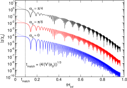
Figure 1: Absolute value $|\chi(t)|$ (solid), and the WKB approximation (dotted) for $H_{\textrm{Inf}}=\phi_{0}=\chi_{0}=10^{12}\,\textrm{GeV}$, $g=1$, $\lambda_{1}=1$, $\lambda_{2}=0.1$, $V_{0}=10^{-4}\rho_{0}^{crit}$, $\xi_{1}=7$ and different values of $\alpha_{0}$. For reasons of clearness the plot has been rescaled by factors $10^{-2}$ and $10^{-4}$ for $\alpha_{0}=\pi/8$ and $0$, respectively. For $\alpha_{0}\not=0$ there is a beat frequency $\omega_{-}/2\equiv(\omega_{1}-\omega_{2})/2$ corresponding to the large oscillations in $|\chi|$, while the fast oscillations of $\chi$ itself are set by $\omega_{+}/2\equiv(\omega_{1}+\omega_{2})/2$.

Thus $\chi_{1,2}(t)$ are both oscillating, but with different frequencies $\omega_{1,2}$ if $\lambda_{2}\not=0$. This leads to a modulation in the phase velocity of the complex field $\chi$ and thus of the comoving asymmetry, which can be calculated using the corresponding expression to Eq. (3) for $\chi$:

$$\begin{array}[]{ll}{\displaystyle A_{\chi}(t)}&{\displaystyle\!\!=\frac{1}{2}\sin(2\alpha_{0})\,\chi_{0}^{2}\,\sqrt{\frac{\omega_{1}(0)\omega_{2}(0)}{\omega_{1}(t)\omega_{2}(t)}}\,e^{{\textstyle-\!\int_{0}^{t}\textrm{d}\tilde{t}\,\Gamma(\tilde{t})}}}\\ &\!\!\times{\displaystyle\left(\omega_{+}\sin\left(\int_{0}^{t}\!\!\textrm{d}\tilde{t}\,\omega_{-}(\tilde{t})\right)-\omega_{-}\sin\left(\int_{0}^{t}\!\!\textrm{d}\tilde{t}\,\omega_{+}(\tilde{t})\right)\right)}\end{array}$$ (12)

with $\omega_{\pm}\equiv\omega_{1}\pm\omega_{2}=(\sqrt{\lambda_{1}+\lambda_{2}}\pm\sqrt{\lambda_{1}-\lambda_{2}})\phi(t)$. Note that only the second part of the damping term $\gamma(t)=3H(t)+\Gamma(t)$ in Eq. (11), which comes from the decay of $\chi$, appears in the asymmetry, while the Hubble term gives a contribution $(a_{0}/a(t))^{3/2}$ which is exactly canceled. Thus, if there was no decay, $\Gamma=0$, the amplitude of the oscillations in the (comoving) asymmetry would stay constant, whereas the frequency increases since the VEV of the quintessence field $\phi$ grows when it rolls down its potential, see the lower graph in Fig. 2. When $\Gamma>0$, the increase in the frequency still occurs, but the amplitude is damped by the exponential term in Eq. (12), see the two upper graphs in Fig. 2. Furthermore, the asymmetry is proportional to $\sin(2\alpha_{0})$, i.e.  it is zero if there is no initial phase difference ($\alpha_{0}=0$), and its modulus is maximal if $\alpha_{0}=\pm\pi/4$.

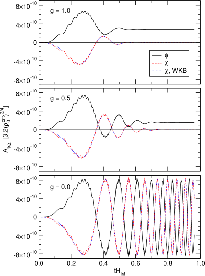
Figure 2: The comoving asymmetries $A_{\phi,\chi}=n_{\phi,\chi}(a/a_{0})^{3}$ in units of $[3.2\,(\rho_{0}^{\textrm{crit}})^{3/4}]$ for $\phi$ (solid), $\chi$ (dashed) and the WKB approximation (dotted, only the leading term proportional to $\omega_{+}$ in the large bracket in Eq. (12) has been kept) for $\alpha_{0}=-\pi/4$ and the other parameters as in Fig. 1. In the two upper graphs the $\chi$ field decays ($g=1,\,0.5$), the lower graph shows the behavior without decay for comparison. In these units, the $B$$-$$L$ asymmetry $n/s$ is the asymptotic value of $A_{\phi}$ for $D=1$ according to Eq. (18).

It is instructive to consider the case when $\lambda_{2}\ll\lambda_{1}$, because then $\omega_{+}^{2}\approx 4\lambda_{1}\phi^{2}\gg\omega_{-}^{2}\approx(\lambda_{2}^{2}/\lambda_{1})\phi^{2}$ and the first term in the large brackets of Eq. (12) dominates, giving the leading oscillations of $A_{\chi}$ with a “low” frequency $\omega_{-}$ proportional to the parameter $\lambda_{2}$, superimposed by a “fast” oscillating component whose amplitude is suppressed by a relative factor $\omega_{-}/\omega_{+}$ (see Fig. 2).

Finally, the analytic expression (12) together with a decay rate of the form $\Gamma(t)=g^{2}/(8\pi)\sqrt{\lambda_{1}}\phi(t)$ can be used to calculate the total asymptotic asymmetry (per comoving volume) $A_{\infty}$ via the integral in Eq. (8):

$$A_{\infty}=\frac{1}{2}\sin(2\alpha_{0})\,\chi_{0}^{2}\,\phi_{0}\sqrt{\lambda_{1}}\frac{g^{2}}{8\pi}\frac{\omega_{+}\omega_{-}}{\Gamma^{2}+\omega_{-}^{2}}\left(1-\frac{\omega_{-}^{2}}{\omega_{+}^{2}}\right)\!\!.$$ (13)

Note that the time-dependence of $\phi(t)$ disappears in the final result and only the initial values $\phi_{0}$ and $\chi_{0}$ enter as dimensionfull quantities. Furthermore, $A_{\infty}$ vanishes if either $\Gamma\propto g^{2}/(8\pi)\rightarrow 0$ or $\lambda_{2}\propto\omega_{+}\omega_{-}\rightarrow 0$ since in these limiting cases no transfer of asymmetry between $\chi$ and the SM, or, respectively, $\chi$ and the quintessence sector would be possible. If, on the other hand, $g^{2}/(8\pi)\approx\lambda_{2}/\lambda_{1}\ll 1$, both transfers are of comparable “strength” and the asymmetry is simply $A_{\infty}\approx\sin(2\alpha_{0})\,\chi_{0}^{2}\,\sqrt{\lambda_{1}}\phi_{0}/2$, independent of $g$ and $\lambda_{2}$. For given initial values $\phi_{0},\chi_{0},\alpha_{0}$ and fixed $\lambda_{1}$, this is the maximum asymmetry that can be transferred.

It turns out that Eq. (13) gives a very accurate estimate for $A_{\infty}$ in the case

$$\phi_{0}^{3}\gg\chi_{0}^{2}\phi_{0},\,\,|V^{\prime}(\phi_{0})|,$$ (14)

since conditions (9) and (10) are both fulfilled from the beginning ($t=0$). This in return can easily be seen from the approximate analytic solution for the quintessence field for early times (when $\phi(t)\ll M_{\textrm{Pl}}$)

$$\phi(t)\approx\phi_{0}+\frac{1}{2}|V^{\prime}(\phi_{0})|t^{2}.$$ (15)

In this domain the asymmetry is independent of $V_{0}$, but (for fixed $\chi_{0}$) only depends on the initial quintessence VEV $\phi_{0}$ (corresponding to the vertical contour lines in Fig. 3).

Figure 3: This contour plot shows the final asymmetry factor $\kappa$ from Eq. (18) for the same parameters as in Fig. 2 ($g=1$) apart from varying values of the initial quintessence VEV $\phi_{0}$ and the initial potential energy $V_{0}$. The light dot-dashed lines divide the plot into three domains: In the right part, due to Eq. (14), $\phi_{0}^{3}\gg\chi_{0}^{2}\phi_{0},\,\,|V^{\prime}(\phi_{0})|$, the asymmetry depends on $\phi_{0}$ but not on $V_{0}$, whereas well inside the upper left part it is vice versa since $|V^{\prime}(\phi_{0})|\gg\phi_{0}^{3},\,\,\chi_{0}^{3}$ from Eq. (16). This is in accordance with the WKB results (20) inside each of these domains. In the remaining part in the lower left corner backreaction effects of $\chi$ on $\phi$ lead to more complex dynamics. Note that $n/s=\kappa D$ with $D=1\dots 10^{-6}$, see Eqs. (18) and (19).

If, on the other hand,

$$|V^{\prime}(\phi_{0})|\gg\phi_{0}^{3},\,\,\chi_{0}^{3},$$ (16)

condition (9) on the phase is actually also satisfied, but condition (10) is only fulfilled for times $t\gtrsim t_{\textrm{match}}\equiv(4/|V^{\prime}(\phi_{0})|)^{1/3}$ as can again be easily seen using (15). To get an estimate of the asymmetry in this case one can use the early-time solution (15) for $t<t_{\textrm{match}}$ and then match the WKB solution for $t>t_{\textrm{match}}$. Since $\phi_{0}t_{\textrm{match}}\ll 1$ (see Eq. (16)) the $\chi$-field can be approximated to stay static until $t_{\textrm{match}}$, and thus the only modification in the WKB results obtained above, especially in the final asymmetry (13), is to replace the initial time $t=0$ by $t=t_{\textrm{match}}$ and

$$\phi_{0}\rightarrow\phi(t_{\textrm{match}})\approx\sqrt[3]{2|V^{\prime}(\phi_{0})|}=\sqrt[3]{2\xi_{1}V_{0}/M_{\textrm{Pl}}}.$$ (17)

In this domain, in contrast to the previous case, the final asymmetry is thus independent of the initial quintessence VEV $\phi_{0}$ and only depends on the initial potential energy $V_{0}$ (corresponding to the horizontal contour lines in Fig. 3).

To determine the final baryon number, we need to calculate the ratio of the produced $B$$-$$L$ asymmetry $n\equiv-A_{\infty}(a_{0}/a)^{3}$ and the entropy density Kolb and Turner (1990),

$$s=\frac{2\pi^{2}}{45}g^{*}(T_{\textrm{R}})T_{\textrm{R}}^{3}\left(\frac{a_{\textrm{R}}}{a}\right)^{3}\approx 3.2\,\rho_{\textrm{R}}^{3/4}\left(\frac{a_{\textrm{R}}}{a}\right)^{3}\!\!\!\!,$$

where $T_{\textrm{R}}$, $\rho_{\textrm{R}}=g^{*}(T_{\textrm{R}})\pi^{2}T_{\textrm{R}}^{4}/30$ and $a_{\textrm{R}}$ are the temperature, energy density and the scale factor at reheating, respectively, and the number $g^{*}(T_{\textrm{R}})$ of active degrees of freedom has been assumed to be of order one hundred. In principle, the final asymmetry of the scenario is independent of the physics between inflation and reheating, however, inflationary dynamics can enter indirectly through the expansion rate when relating the corresponding scale factors and critical energy densities via

$$\rho_{\textrm{R}}^{3/4}a_{\textrm{R}}^{3}=(\rho_{0}^{\textrm{crit}})^{3/4}a_{0}^{3}\exp[{\textstyle\frac{3}{4}\int_{0}^{t_{\textrm{R}}}\textrm{d}t\,H(t)(1-3\omega(t))}],$$

where $\omega(t)$ is the equation of state parameter of the dominant component, i.e.  the inflaton and later radiation. Thus the final asymmetry relative to the entropy density is given by

$$\frac{n}{s}=\underbrace{\frac{-A_{\infty}}{3.2(\rho_{0}^{\textrm{crit}})^{3/4}}}_{\equiv\,\kappa}\,\underbrace{\exp\left({\displaystyle-\frac{3}{4}\int_{0}^{t_{\textrm{R}}}\!\textrm{d}t(1-3\omega(t))H(t)}\right)}_{\equiv\,D}\!\!.$$ (18)

The first factor $\kappa$ depends only on the dynamics of the quintessence and the mediating field shortly after inflation, whereas the second factor $D$ describes the dilution of the asymmetry between the end of inflation and the time when $\omega(t)\rightarrow 1/3$. In fact, $1/D$ is equal to the spatial expansion of the universe after inflation relative to a radiation dominated cosmos. Note that the upper limit in the integration can be formally extended beyond reheating, since from then on $\omega=1/3$. This makes it obvious that any inflationary scenario can only have an impact on the final baryon number through its equation of state and not through further characteristics, e.g. the reheating temperature.

To get a plausible range for $D$ we will consider various possibilities: for example, if the inflaton field $I$ oscillates in a potential of the form $I^{m}$ with even $m$, its mean equation of state (averaged over a whole oscillation period) is $\omega=\frac{m-2}{m+2}=\textrm{const}$ Shtanov et al. (1995). Assuming that this is true for the whole time between the end of inflation and reheating we get $D=(2.4\,T_{\textrm{R}}/(\rho_{0}^{\textrm{crit}})^{1/4})^{(4/m-1)}$. For $T_{\textrm{R}}=10^{9}\,\textrm{GeV}$, $H_{\textrm{Inf}}=10^{12}\,\textrm{GeV}$ and $m=2$ this gives $D\approx 10^{-6}$, whereas for $m=4$ there is no dilution at all yielding $D=1$, with or without preheating Shtanov et al. (1995). Another example is a model with preheating and a quadratic minimum ($m=2$) for the inflaton. For the case recently discussed in Ref. Podolsky et al. (2005), one finds $D\approx 10^{-1}\dots 10^{-3}$. Here we will adopt the point of view that the dilution factor $D$ will be roughly in the range $1\dots 10^{-6}$, yielding a range for $\kappa$

$$10^{-10}\lesssim\kappa\lesssim 10^{-4},$$ (19)

that is compatible with the observed value $n/s\sim 10^{-10}$ Spergel et al. (2003). Using the analytic estimates (13) and (17) one obtains

$$\kappa\approx-\frac{\mathcal{N}}{2}\sin(2\alpha_{0})\left(\frac{\chi_{0}}{H_{\textrm{Inf}}}\right)^{\!2}\!\!\times\left\{\begin{array}[]{l}\frac{\phi_{0}}{7.3H_{\textrm{Inf}}}\left(\frac{H_{\textrm{Inf}}}{M_{\textrm{Pl}}}\right)^{3/2}\\ \frac{1}{4}\left(\frac{\xi_{1}V_{0}}{\rho_{0}^{\textrm{crit}}}\right)^{1/3}\left(\frac{H_{\textrm{Inf}}}{M_{\textrm{Pl}}}\right)^{7/6}\end{array}\right.$$ (20)

with $\mathcal{N}\equiv\frac{g^{2}\sqrt{\lambda_{1}}}{8\pi}\frac{\omega_{+}\omega_{-}}{\Gamma^{2}+\omega_{-}^{2}}(1-\omega_{-}^{2}/\omega_{+}^{2})$. The upper and lower line of Eq. (20) correspond to the cases (14) and (16), respectively. For coupling constants $g^{2}/(8\pi)\sim\lambda_{2}/\lambda_{1}\ll 1\sim\lambda_{1}$, $\mathcal{N}$ is of order one. Generically assuming $\sin(2\alpha_{0})\sim-1$ and $\chi_{0}\sim H_{\textrm{Inf}}\sim 10^{12}\,\textrm{GeV}\sim 4\cdot 10^{-7}M_{\textrm{Pl}}$ we thus find values for $\kappa$ of roughly $10^{-11}\phi_{0}/H_{\textrm{Inf}}$ and $10^{-8}(V_{0}/\rho_{0}^{\textrm{crit}})^{1/3}$ respectively, which lie inside the allowed range (19) for a huge variety of initial conditions of the quintessence VEV and its potential energy after inflation (see Fig. 3).

IV Fermionic couplings

There are various possibilities to couple the mediating field $\chi$ of our toy model to the fermionic sector for which we will give two examples in this section.

Since the whole scenario is $B$$-$$L$ conserving, the right-handed neutrinos do not have a Majorana mass term and carry lepton number one. As the $\chi$-field is also a gauge singlet it can be coupled to one (or more) right-handed neutrino(s) $N$ via

$$g\,\overline{N^{C}}N\chi+\mbox{h.c.}.$$ (21)

This would assign the desired lepton number to the $\chi$ field and implies the given decay term $\Gamma\dot{\chi}$ in the equation of motion (6). However, if this was the only additional coupling, the asymmetry would remain stored in the right-handed neutrino sector due to their tiny Yukawa couplings Dick et al. (2000). In this case one would have to find a way to transfer the lepton asymmetry to the SM sector, where sphalerons could create the final baryon asymmetry. This could be realized by a light scalar field $S$ (with mass $H_{\textrm{Inf}}\gg m_{S}\gtrsim\rm{TeV}$) with the same quantum numbers as the SM Higgs field and a quadratic potential. If this scalar would start with a typical VEV of order $H_{\textrm{Inf}}$ at the end of inflation, it would remain frozen in until $H$ drops below the mass of the scalar. In this case an additional coupling term

$$g^{\prime}\,\overline{\ell}NS+\mbox{h.c.}$$ (22)

with a left-handed lepton doublet $\ell$ and suitable coupling constant $g^{\prime}$ should lead to the required left-right-equilibration of the neutrinos as $H$ becomes smaller. When $H$ drops below the mass of the scalar the VEV of $S$ would start oscillating and finally vanish. It might even be possible to avoid the introduction of such a new particle by introducing a similar coupling between the inflaton and the neutrinos. In this latter case one would get additional constraints for the inflationary scenario.

One possibility, which works without the introduction of additional particles while also being independent of the inflationary model, would be to couple the $\chi$ field directly to the left-handed neutrinos $\nu$ via the term

$$g\,\overline{\nu^{C}}\nu\chi+\mbox{h.c.}.$$ (23)

Due to the heavy mass of $\chi$ this should be consistent with observations. However, the explicit breaking of gauge invariance makes this option less attractive.

V Stability and Q-Balls

In this section we discuss possible sources of instability in our model. For instance, particle processes and spatial inhomogeneities could disturb the scalar field evolution described in the previous sections. One peculiarity of complex scalar fields with a conserved global quantum number is the potential formation of so-called Q-Balls Coleman (1985). A Q-Ball is a non-topological soliton and represents a spatially extended scalar field configuration carrying a non-zero charge associated to the global symmetry. For our scenario it is essential that the complex quintessence field does not promote the formation of Q-Balls, which could make the field unstable and inhomogeneous and thereby destroy its DE properties. To analyze the stability of the scalar fields in our model one has to to solve the corresponding equations of motion including the spatial derivatives that were omitted in Eqs. (5) and (6). Since the numerical solution of this system of partial differential equations is beyond the scope of this paper (see e.g. Kasuya and Kawasaki (2001)), let us instead proceed with a much simpler approach that might give us at least some hints towards the stability properties of our model. Since we also only want to show that instabilities should not be a problem for our model in general, we only consider the initial conditions and parameter values as in Fig. 1 ($g=1$) and neglect perturbations in the metric.

Following Refs. Kusenko and Shaposhnikov (1998); Kasuya (2001) we study the evolution of small inhomogeneous perturbations in the scalar fields. Substituting $\phi(x,t)\rightarrow\phi(t)+\delta\phi(x,t)$ and $\chi(x,t)\rightarrow\chi(t)+\delta\chi(x,t)$, where the first parts denote the homogeneous solutions of the previous sections, we can derive the equations of motion for $\delta\phi$ and $\delta\chi$ from the Lagrangian (II). Keeping only the terms linear in the small perturbations, we find a mass mixing matrix for $\delta\phi$ and $\delta\chi$, where the dominating contributions on the main diagonal, at early times, are of the order $V^{\prime}(|\phi|)/|\phi|$ and $\lambda_{1}|\phi|^{2}$ for $\delta\phi$ and $\delta\chi$, respectively, while the off-diagonal terms are of the order $\lambda_{1}\chi\phi$. As we checked numerically, the off-diagonal entries never become solely dominant, therefore we will consider the perturbations of $\phi$ and $\chi$ separately in this simplified analysis.

Now, we write the complex scalars $\phi$ and $\chi$ in the form $\phi=\varphi e^{i\theta}$, $\chi=|\chi|e^{i\sigma}$ with real functions $\varphi$, $\theta$ and $\sigma$. Within the quintessence field $\phi$ we consider perturbations of the type $\delta\varphi=\delta\varphi_{0}\exp(\Omega(t)+i\vec{k}\vec{x})$, $\delta\theta=\delta\theta_{0}\exp(\Omega(t)+i\vec{k}\vec{x})$, that are characterized by a wavenumber $k=|\vec{k}|$ and a time-dependent function $\Omega(t)$. From the Lagrangian (II) we derive the equations of motion for the quintessence field

$$0 = \ddot{\varphi}+3H\dot{\varphi}-a^{-2}\nabla^{2}\varphi-\varphi\dot{\theta}^{2}+a^{-2}\varphi(\nabla\theta)^{2}$$ (24)

$$+ V^{\prime}(\varphi)+|\chi|^{2}\varphi[\lambda_{1}+\lambda_{2}\cos 2\alpha],$$

$$0 = \ddot{\theta}+3H\dot{\theta}-a^{-2}\nabla^{2}\theta+2\dot{\theta}{\textstyle\frac{\dot{\varphi}}{\varphi}}$$ (25)

$$- 2a^{-2}(\nabla\varphi)(\nabla\theta)-\lambda_{2}|\chi|^{2}\sin 2\alpha,$$

where $\alpha=\theta-\sigma$ is the phase difference of both scalar fields. By substituting $\varphi\rightarrow\varphi+\delta\varphi$, $\theta\rightarrow\theta+\delta\theta$ and keeping only terms at most linear in the perturbations $\delta\varphi$, $\delta\theta$, one obtains a system of equations for $\delta\varphi$ and $\delta\theta$. The condition for this system to have a non-trivial solution reads

$$0 = \left(\ddot{\Omega}+\dot{\Omega}^{2}+3H\dot{\Omega}+{\textstyle\frac{k^{2}}{a^{2}}}-\dot{\theta}^{2}+V^{\prime\prime}(\varphi)\right.$$ (26)

$$+ |\chi|^{2}[\lambda_{1}+\lambda_{2}\cos 2\alpha]\Big{)}\times\left(\ddot{\Omega}+\dot{\Omega}^{2}\right.$$

$$+ \left.3H\dot{\Omega}+{\textstyle\frac{k^{2}}{a^{2}}}+2\dot{\Omega}{\textstyle\frac{\dot{\varphi}}{\varphi}}-2\lambda_{2}|\chi|^{2}\cos 2\alpha\right)$$

$$+ 4\dot{\theta}\left(\dot{\Omega}\dot{\theta}+\lambda_{2}|\chi|^{2}\sin 2\alpha\right)\times\left(\dot{\Omega}-{\textstyle\frac{\dot{\varphi}}{\varphi}}\right)\!.$$

If this equation for $\Omega(t)$ has any solution with $\textrm{Re}(\dot{\Omega})>0$ for a period of time, then the perturbation mode $\sim\exp(\Omega(t)+i\vec{k}\vec{x})$ is growing exponentially, possibly indicating an instability in the scalar field $\phi$, which could lead to the formation of Q-Balls. The following discussion is divided into three parts. First, during the early moments of evolution, when the mediating field $\chi$ has not yet decayed, we will study the stability of the model mainly numerically. The second and third parts concern the time directly after the $\chi$-decay and the very late cosmological era, respectively, where we can now treat the problem completely analytically.

Starting at the end of inflation we solve Eq. (26) numerically for the function $\dot{\Omega}(t)$ and several different choices of the wavenumber $(k/a)^{2}$ and the initial phase difference $\alpha_{0}$. In some cases one can observe positive values of $\textrm{Re}(\dot{\Omega})$, which appear maximal for small $k$. As an example the $k=0$ case is shown in Fig. 4. However, for these unstable modes, $\textrm{Re}(\dot{\Omega})$ turns out to be much smaller than the Hubble scale $H_{\textrm{Inf}}$ so that there is not enough time for the instabilities to develop. In addition, a wavenumber smaller than $H_{\textrm{Inf}}$ implies that the wavelength of the perturbation is larger than the Hubble radius and its evolution is therefore suppressed by the cosmological expansion. For modes with large wavenumbers $(k/a)^{2}\gg H_{\textrm{Inf}}^{2}$ the numerical solutions of Eq. (26) do not show growing perturbations, as expected.

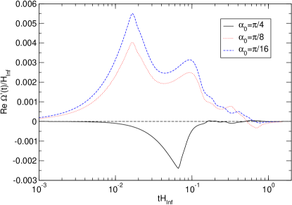
Figure 4: The real part of $\dot{\Omega}(t)$, where the function $\Omega(t)$ describes the evolution of the inhomogeneous perturbations $\delta\varphi,\delta\theta\propto\exp(\Omega(t)+i\vec{k}\vec{x})$ for different values of the initial phase difference:  $\alpha_{0}=\pi/4$, $\pi/8$, $\pi/16$. For this numerical solution the wavenumber $(k/a)$ and the initial value of $\dot{\Omega}$ are taken to be $0$. The remaining parameters are the same as in Fig. 1.

To study the late-time behavior of the inhomogeneities, we simplify Eq. (26) by neglecting $|\ddot{\Omega}|\ll|\dot{\Omega}^{2}|$, i.e. assuming a slowly changing $\omega\equiv\dot{\Omega}$ since the background solution is now slowly varying. In addition the mediating field $\chi$ has already decayed ($|\chi|=0$). Thus, we obtain

$$0 = \left(\omega^{2}+3H\omega+{\textstyle\frac{k^{2}}{a^{2}}}-\dot{\theta}^{2}+V^{\prime\prime}(\varphi)\right)$$ (27)

$$\times \left(\omega^{2}+3H\omega+{\textstyle\frac{k^{2}}{a^{2}}}+2\omega{\textstyle\frac{\dot{\varphi}}{\varphi}}\right)+4\omega\dot{\theta}^{2}\left(\omega-{\textstyle\frac{\dot{\varphi}}{\varphi}}\right)\!\!,$$

where solutions with a positive real part of $\omega$ might indicate an instability. We find that the range of values for the wavenumber $k/a$ that solves this equation for $\textrm{Re}(\omega)>0$ is given approximately by

$$0<\left(\frac{k}{a}\right)^{\!2}\lesssim\left(\frac{k_{\textrm{max}}}{a}\right)^{\!2}\!\equiv\dot{\theta}^{2}-V^{\prime\prime}(\varphi).$$ (28)

Hence, the late-time evolution of the quintessence field is stable for $\dot{\theta}^{2}\lesssim V^{\prime\prime}(\varphi)$. To verify this condition let us assume for the comoving asymmetry of the quintessence field a maximal value of $|A_{\phi}|=2|\dot{\theta}|\varphi^{2}(a/a_{0})^{3}\sim 10^{-8}(\rho_{0}^{\textrm{crit}})^{3/4}$, where the initial critical energy density is given by $\rho_{0}^{\textrm{crit}}\sim H_{\textrm{Inf}}^{2}M_{\textrm{Pl}}^{2}$. Although $\varphi$ starts with the value $\varphi_{0}\sim H_{\textrm{Inf}}$, it quickly reaches the Planck scale $M_{\textrm{Pl}}$, therefore we take the moderate value $\varphi\sim\sqrt{H_{\textrm{Inf}}M_{\textrm{Pl}}}$ at early times so that

$$|\dot{\theta}|\sim 10^{-8}\,\frac{(\rho_{0}^{\textrm{crit}})^{3/4}}{\varphi^{2}}\left(\frac{a}{a_{0}}\right)^{\!-3}<10^{-8}\sqrt{H_{\textrm{Inf}}M_{\textrm{Pl}}}.$$ (29)

Even if we now choose the low value $V_{0}\sim H_{\textrm{Inf}}^{3}M_{\textrm{Pl}}$ in the quintessence potential $V(\varphi)=V_{0}e^{-\xi_{1}\varphi/M_{\textrm{Pl}}}$, we obtain

$$\frac{\dot{\theta}^{2}}{V^{\prime\prime}(\varphi)}<10^{-16}\frac{M_{\textrm{Pl}}^{2}}{\xi_{1}^{2}H_{\textrm{Inf}}^{2}}\sim 10^{-4}\ll 1,$$ (30)

where we used $H_{\textrm{Inf}}\sim 10^{-7}\,M_{\textrm{Pl}}$ and $\xi_{1}\sim 10$. At very late times in the cosmological evolution with a low Hubble scale $H\ll H_{\textrm{Inf}}$ we find $V^{\prime\prime}(\varphi)=\mathcal{O}(H^{2})$ Steinhardt et al. (1999), $\varphi\gtrsim M_{\textrm{Pl}}$ and $(a/a_{0})^{-3}=(H/H_{\textrm{Inf}})^{3/2}$ for a long period of radiation dominance. Thus, the quintessence field is also stable in this epoch:

$$\frac{\dot{\theta}^{2}}{V^{\prime\prime}(\varphi)}\sim 10^{-16}\frac{H}{M_{\textrm{Pl}}}\ll 1.$$ (31)

We conclude that the quintessence scalar field in our scenario does not seem to suffer from instabilities, at least within the context of this simplified analysis. In principle, we could perform a similar analysis also for the mediating field $\chi$. However, since it decays into neutrinos very quickly, a possible instability of $\chi$ should not harm our scenario. Additionally, Q-Balls built from this field could also decay into leptons Cohen et al. (1986); Multamaki and Vilja (2000); Clark (2005). For a deeper discussion of Q-Balls see e.g.  Ref. Enqvist and Mazumdar (2003) and the references therein.

In the last part of this section we want to motivate the statement that particle processes only enter the equations of motion of the fields in form of the decay term $\Gamma\dot{\chi}$ in Eq. (6) and make it plausible that this might even hold within a full quantum-mechanical treatment of the quintessence field. However, one has to admit, that such a treatment of the quintessence field would go far beyond the scope of this paper and more subtleties would arise than the ones mentioned here.

Still, we notice that one could also allow additional particle processes like the one in Fig. 5, which might destabilize the $\phi$ condensate.

Figure 5: Example for an additional process between $\phi$ and the leptonic sector.

However, even if this was done it is unlikely that they would have a large impact on the scenario due to the following arguments. We first notice that at the beginning of the scenario the masses of the scalar particles (proportional to the second derivative of the corresponding potential) are of the order of $H_{\textrm{Inf}}$ or smaller. By dimensional analysis the reaction rates $\Gamma_{i}$ for the mentioned processes should therefore be of the same order of magnitude at this time (assuming coupling constants to be of order one). However, before the corresponding time elapses the mass of $\chi$ has increased by several orders of magnitude. Since these masses appear in the denominator of the reaction rates the ratio $\Gamma_{i}/H$ will now always be smaller than one and the reaction should never have enough time to take place as also resonances do not seem to occur.

We also note that additional decay channels of $\chi$ would not harm our scenario as long as the lepton asymmetry is transferred to SM particles before the electroweak phase transition. A decay channel which could potentially be dangerous is a decay into hypothetical quanta of the quintessence field, if they represent physical degrees of freedom, via the couplings of the form $\lambda_{1,2}\phi^{2}\chi^{2}$. However, a simple estimate for the decay rate $\Gamma_{2\chi\rightarrow 2\phi}\approx\lambda_{1,2}^{2}|\chi|^{2}/(8\pi m_{\chi})$ Dolgov (1992) shows that it is both suppressed by the increase of $m_{\chi}$ and the decrease of $|\chi|$ as compared to the rate $\Gamma_{\chi\rightarrow 2\nu}=g^{2}m_{\chi}/(8\pi)$ for the decay into neutrinos.

VI Summary and Conclusions

In this work we have proposed a $B$$-$$L$ conserving baryogenesis scenario, in which a $B$$-$$L$ asymmetry is hidden in the DE sector. This is achieved by the introduction of two complex scalar fields carrying lepton number, where one of them is responsible for DE in a quintessence-like manner while the other one mediates between this field and the SM particles (including right-handed neutrinos). An initial phase difference between the VEVs of these two fields results in compensating but non-zero lepton asymmetries for them. While the quintessence field has a tracking behavior, the mediating field acquires a large mass and eventually decays, hereby transferring its asymmetry to the fermionic sector. Finally sphalerons partially transform this lepton asymmetry to a baryon asymmetry. We quantitatively determined the resulting baryon asymmetry numerically and also gave an analytic formula based on a WKB approximation. Both results are consistent and show that the observed value can easily be achieved. Furthermore, we have analyzed potential sources of instability like Q-Ball formation and did not find any hints for an unstable behavior.

Of course, a deeper understanding of several topics is desirable. A thorough knowledge about the VEVs of scalar fields after inflation, especially in the case of complex potentials, could help to restrict the parameter space of our model immensely. Also, as stated before, a full quantum-mechanical treatment of the quintessence field is wish-full. This could enable us to further restrict the couplings in our scenario, while it might also make way for new baryogenesis models in which the quintessence field is directly coupled to SM particles.

The possible $B$$-$$L$ quantum numbers of the vacuum could also have interesting consequences for additional couplings between DE and SM fields or dark matter. Moreover quantum numbers of the quintessence field could include hints at its origin.

In conclusion, we presented a specific model that leads to the observed baryon asymmetry of the universe with a strict conservation of $B$$-$$L$ and the storage of a corresponding asymmetry in the DE sector.