hep-ph/0510332

CPHT-RR 063.1005

LTH 678

On the Effective Theory of Low-Scale Orientifold String Vacua

Claudio Corianò ^1,2,  Nikos Irges ³ and Elias Kiritsis ^3,4

¹Dipartimento di Fisica, Università di Lecce, and
INFN Sezione di Lecce, Via Arnesano 73100 Lecce, Italy

² Department of Mathematical Sciences, University of Liverpool
Liverpool L69 3BX, U.K.

³Department of Physics, University of Crete, 71003 Heraklion, Greece

⁴CPHT, Ecole Polytechnique, UMR du CNRS 7644, 91128, Palaiseau, FRANCE

The effective field theory of the minimal Low Scale Orientifold Models is developed. It describes universal features of related orientifold vacua in string theory. It contains, beyond the Standard Model fields, an MSSM-like Higgs sector and three anomalous (massive) U(1) gauge bosons. All renormalizable couplings are included as well as some dimension-five couplings that are important for anomaly cancellation. The Higgs symmetry breaking induces mixing between the anomalous U(1) gauge bosons and the photon and $Z^{0}$. This mixing as well as the anomaly generated cubic vector boson couplings is potentially important for discriminating such models from other theories containing Z’s. Some interesting tree-level processes are also evaluated.

1 Introduction

String theory owes its popularity and promise to the fact that it includes consistently gravity along with other gauge interactions. The most explored set of vacua in string theory have a string scale that is close to the four-dimensional Planck scale. All successful heterotic vacua, whether perturbative, or M-theoretic have this property. This is appealing due to indications from running coupling unification. On the other hand, no simple reliable predictions are possible without a detailed vacuum, that is sufficiently close to the Standard Model (SM) at low energy. Although there are some heterotic vacua that come close [1, 2], it is fair to say that none so far has passed all tests in a controllable fashion. Moreover, to put it simply, it is hard to see string effects at $E\sim 1$TeV when $M_{s}\sim 10^{13}$ TeV.

In the past decade, other perturbative vacua of string theory have been explored. A particularly interesting class are orientifold vacua [3, 6, 7], that in their broad sense are compactifications of the type I string. Their generic structures involves a compact six dimensional manifold or orbifold thereof, times a Minkowski space. The more general option, relevant in the presence of fluxes may warp Minkowski space. The internal space is threaded with D_p≥3 branes and Orientifold planes that stretch along Minkowski space and have their potential extra dimensions wrapped around cycles of the internal manifold.

Because of this, there is no direct link between the string scale and the four-dimensional Planck scale. By adjusting (if possible) the internal volumes any possible number for $M_{s}<M_{P}$ can be obtained [8, 9]. Of course, especially in the absence of supersymmetry, volumes along with other moduli acquire potentials, and their values are determined dynamically. It has been argued that there may be vacua where the string scale could be as low as 1 TeV although to the present day, no reliable such vacuum exists.

There has been quite a bit of success though in model building so far with a high string scale (see [10, 11, 12] and references therein), although, as in the heterotic case, there is no perfect vacuum yet.

Low scale string vacua, have the undeniable charm that there may be amenable to experimental tests. Even though, as already stated, there may be no such model at present solving the tadpoles conditions, their general structure has characteristic features, and experimental signals that are essentially generic. The purpose of the present work is to formulate and parameterize the generic low energy action of the most interesting class of such vacua, that we call minimal Low Scale Orientifold Models or mLSOM for short. Such an effective action can help both the string theory search for such vacua, currently under way [14], as well as the parametrization and computation of experimental observables.

Orientifold vacua have a conceptual simplification build in: there is a clear separation typically between the open string spectrum, coming from the D-branes, and the “bulk” spectrum coming from the unoriented closed strings. The graviton is part of the bulk spectrum, whereas the branes give rise to particles at the massless sector with spin at most one.

The standard model gauge group and other particles is naturally realized on the D-branes rather than the bulk. There are several reason for this. A simple and powerful one is that it is not possible to realize the non-abelian structure of the SM including its reps in type II string theory [15]

The gauge group coming from the D-branes is a product of classical but not exceptional groups, each factor coming from a stack of branes at the same point in transverse space. The minimal gauge groups that can accommodate the standard model particles are U(3)$\times$U(2)$\times$U(1), and U(3)$\times$U(2)$\times$U(1)$\times$U(1)’ [16, 18, 19]. There are variants where U(2)$\to$Sp(2)$\sim$SU(2), and U(1)$\to$O(2). There will be in general a hidden group, that for the whole paper we will neglect, although it may be important (depending on the model) for issues of supersymmetry breaking. Of course one may consider more complicated groups. The Pati-Salam like group U(4)$\times$U(2)² is the simplest example. However unlike field theory, here the minimal groups are more advantageous, since the larger ones must be eventually broken and we should be able to describe them directly in their broken phase.

There is an obvious observation: all such embeddings involve U(1) factors that are more numerous than what we know in the SM, namely the hypercharge [16]. It is also known that many U(1)’s can be anomalous in orientifolds [20]. Anomalies cancel, although the appropriate charge traces are non-zero, thanks to variants of the Green-Schwarz mechanism [21]. It is known that anomalous U(1)s become eventually massive, and the associated gauge symmetry is broken. Under certain conditions, the global symmetry may remain unbroken in perturbation theory (see [22] for a review). It is then hoped that all extra U(1)’s except the hypercharge become hopefully massive. In fact, this is generically the case.

The anomalous U(1) masses, can be calculated unambiguously via a one-loop (annulus) computation [23, 24, 25]. A rich pattern of masses appears. It turns out that the physical masses are bounded above by the string scale, but can be arbitrarily low, if some internal dimensions are large. In the generic case however they turn out to be a few times smaller than $M_{s}$, if one includes, $\pi$’s and i’s.

In fact, the anomalous U(1)’s gauge bosons have essentially all their renormalizable couplings fixed by charges and anomalies. Apart from their minimal couplings, they mix with appropriate bulk axions, that couple to other gauge fields via PQ-type couplings. They also have most of the time, cubic Chern Simons-like interactions due to anomalies [28]. The effective cubic couplings together with the non-zero triangle diagrams, provide an effective cubic vertex to the anomalous U(1)s gauge bosons. This effect is absent from usual non-anomalous Z’s. They may have therefore signals that distinguish them from other Z’ candidates, [29, 30, 31]. Moreover, due to the fact that the Higgs is always charged under such anomalous U(1)’s the Z’s mix with the $Z^{0}$ gauge boson. Therefore, the photon and the $Z^{0}$ acquire a (suppressed) cubic vertex.

If the string scale is in the TeV range, such anomalous U(1)’s are prime candidates for detection. At the same time, they provide many contributions to known processes, that could exclude ranges of the parameters (Z-couplings [32],[33], [34] and $g-2$ [35] being two examples that have been partially studied so far).

Apart from the SM spectrum and the anomalous U(1) gauge bosons, there are other low-energy particles in the orientifold vacua with low string scale. We will enumerate them below and describe briefly their characteristics.

• Additional Higgses. Higgses typically come in pairs, even if supersymmetry is broken at the string scale. The large scale study of [36] based on the hypercharge embedding of [37], [38], shows that there are different vacua with a variable number of doublets. Of course there should be at least one. And for simplicity we assume that there are no others around.

• Superpartners of the SM particles. Depending on the way supersymmetry is broken, they may have masses that are well below, to around the string scale. In fact, in low scale orientifold models, the most natural way of breaking supersymmetry is the “ explicit breaking” which gives $M_{s}$ as the susy breaking scale. In such a case the partners have masses at the string scale and they are typically heavier than the anomalous U(1) gauge bosons, with the possible exception of the higgsinos.

• Non-chiral massless states. There are no such states in the SM therefore they must be somehow lifted in mass. It is possible, combining intersecting branes with Scherk-Schwarz deformations to actually remove all such states from the massless spectrum [39].

• Possible hidden groups, encompassing all other massless-level open string states that do not directly interact (by construction) with the SM particles.

• Open string KK-states. Some of the branes may wrap internal dimensions. As explained in [17], when the string scale is low, the most advantageous configuration has two large dimensions. All others have size at most twice the string length. Moreover all SM particles wrap the small dimensions. Therefore, their KK states have masses at the string scale. There are two exceptions. The first is when one of the branes wraps the two large dimensions. The associated anomalous gauge boson, on the other hand is massive, and it should be arranged that the mass comes from N=2 sectors so that it is of the order of the string scale [17]. Therefore although its KK states are very tightly spaced, its zero point mass is large. It is interesting that this type of massive gauge boson, might have a very particular signal at LHC, because of this very special property.

  The second exception concerns the KK states of the right-handed neutrinos that come from the above described brane. These mix with the zero modes and provide an interesting pattern of masses. This was analyzed in [17].

• Stringy states of open strings. All the states above have stringy excitations (vibration modes) of the associated open strings with masses at the string scale and above.

• Massless bulk modes, including the graviton, having gravitational strength couplings to the open sector. After the breaking of susy, all but the graviton should acquire masses.

• Bulk KK states. Since there are two compactification scales, the one that dominates at low energy is associated to the two larger dimensions. The physics of such KK states has been analyzed in the past [40]

• Bulk stringy states, with masses at the string scale or more.

Typically, apart from the SM particles, the particles that are lightest from the brane particles, are firstly the anomalous U(1) gauge bosons and then superpartners. The distribution of masses depends on the vacuum. In this paper, we will neglect superpartners, since this is a well studied sector. We will focus on the anomalous U(1) gauge bosons, the Higgses and the SM particles. The bulk axions that are crucial for anomaly cancellation will also be included.

In successful low scale orientifold vacua, baryon and lepton number are gauge symmetries. They are in fact some of the anomalous U(1)s. Their gauge bosons will become massive but the associated global symmetries will remain intact in perturbation theory. This is a crucial fact , since at low $M_{s}$ baryon and lepton number violating operators will be hardly suppressed, [41]. There will be breaking due to instantons but this is known to be small.

This general class of models has important open problems that need to be eventually addressed at the string level, in order to have concrete successful string vacua that realize this setup.

• The setup needs radii much larger than the string scale. This hierarchy, leading to a low string scale must be explained/accomodated.

• It must be arranged that the PQ symmetry is explicitly broken, in order to avoid a massless axion.

• The problem of one-loop tadpoles needs to be accommodated somehow.

There are several important effects, in the effective theory we are describing. A crucial ingredient is that in all cases, the Higgs gauge bosons are charged under one linear combination of the anomalous U(1)s. In fact we can go to a basis (a non-orthogonal one) where the four generic U(1) symmetries of the low scale orientifold vacua are hypercharge, Y, baryon number B, lepton number, L, and a Peccei-Quinn-like symmetry PQ. The Higgs then has B=L=0, and its vacuum expectation value breaks Y and PQ.

The UV mass matrix of the U(1) gauge bosons is characterized by three mass eigenvalues of order $M_{s}$, (hypercharge is massless) as well as three mixing angles. The second source of gauge boson masses is the Higgs symmetry breaking. Due to the (mild) hierarchy of the Higgs vev and $M_{s}$ there is interesting pattern in the gauge boson mass-eigenstates.

The photon is the usual mixture of Y and $W^{3}$. However, the $Z^{0}$, apart from its Y and $W^{3}$ components, it has a small ($\sim{\cal O}(M^{2}_{Z}/M^{2}_{s})$) admixture of the other three anomalous U(1) gauge bosons. Similarly, the three heavy $Z^{\prime}$s have a small admixture of Y,$W^{3}$. The presence of this mixing affects in an interesting way several issues:

• $Z^{0}$ has non-standard couplings to fermions. This also affects the $\rho$ parameter.

• $\gamma$ and $Z^{0}$ acquire a trilinear vertex, an avatar of their mixing to the anomalous U(1)s and the triple anomalous U(1) vertex. This is very interesting for LHC.

• There are non-standard photon and $Z^{0}$ couplings to the Higgs.

It is these issues that we will analyse to a certain extent in the present paper.

We should also briefly mention the parameters of the effective field theory. We do have, to start with, all the SM parameters.

The Higgs sector resembles that of the MSSM, in the sense that it has two Higgses. However, if supersymmetry is broken at the string scale, the structure of the potential at the level of the quadratic terms maybe different. It depends in fact on the way supersymmetry is broken. However for orbifold and SS breaking the tree level potential is of the supersymmetric type. However, in this paper, for generality we will keep all possible terms.

We split the terms in the Higgs potential into those that preserve the PQ symmetry and those who do not. The PQ-preserving part has four real quartic couplings and two quadratic ones. The PQ-breaking part has one complex quadratic coupling and three complex quartic ones. It is essential for giving a mass to an otherwise massless scalar, the axi-Higgs, a mixture of one if the Higgs phases and the bulk axions.

The anomalous U(1) sector has a 4$\times$4 UV mass matrix that is generically not diagonal. One of its eigenvalues is zero corresponding to the hypercharge. The hypercharge linear combination is fixed by a set of integers. For mLSOM, there are two choices. The rest of the matrix can be parameterized in terms of three mass eigenvalues and three mixing angles. The axion-gauge boson mixing, axion-gauge boson CP-odd couplings as well as the CS-like couplings are then determined in terms of the mass matrix and the charges, that are known.

One of the anomalous U(1) gauge bosons comes from a brane that wraps the two large dimensions [16]. This implies that its UV mass term as well as the mixing terms with the other U(1) gauge bosons should be anywhere between $M_{s}$ and $\sim 10^{-3}$ eV. We will assume in this paper, for simplicity that its mass comes from an N=2 sector and therefore its physical mass is of the order of the string scale. In any case, its mass must be larger than around 50 MeV to avoid standard supernova cooling constraints [17].

In the neutrino sector that is not discussed in this paper, there are further parameters that enter. If there is a single bulk right handed neutrino then there are three parameters associated to its coupling to the three lepton doublets. If there are three bulk neutrinos, then one has the standard KM-like mixing matrix. On top of this there is neutrino mixing with the right-handed neutrino KK modes that are densely spaced. In the simplest uniform case of a $T^{2}$ with the same radius, it is the radius that enters as an new parameter (constrained at the same time by fitting the gauge couplings and the Planck scale.) These issues are discussed in detail in [17]. In the sequel we choose the innocuous case of three bulk neutrinos and neglect the mixing with the KK states.

The structure of this paper is as follows: In section 2 we describe the string theory origin of the effective field theories that we analyze. They should correspond to string theory vacua with a string scale in the TeV range.

In section 3 we describe the effective action under study. We describe in detail the UV (stringy) gauge boson mass terms, and we also describe convenient gauge fixings in the unbroken phase.

In section 4 we analyze in detail the issue of electroweak symmetry breaking. This is of importance as the properties of Z’s are affected importantly. We discuss in particular, the gauge boson masses the structure of the Higgs sector, the details of the Green-Schwarz sector responsible for anomaly cancellation and finally a convenient gauge-fixing in the broken phase.

Section 5 contains the computation of various tree level cross sections that are relevant for constraining the parameter space and analyzing new physics in this class of models.

Finally 6 contains our conclusions and further comments.

Appendix A contains a comparison of the Higgs sector here with the SM Higgs sector while appendix B contains a rewriting of the Lagrangian in the physical basis.

2 String theory origin of the mLSOM

In this section we motivate the type of effective theory we will be studying in this paper, by linking it to a class of interesting vacua of string theory. These are known as orientifold vacua. Useful reviews introducing this subject and describing recent progress can be found in [10]-[13].

The generic structure is as follows. The ten dimensions of superstring string theory are split into four flat non-compact dimensions and six compact dimensions, threaded with other possible background fields (tensor fluxes). Several groups of D_p≥3-branes are inserted in this vacuum, so that their 3+1 dimensions are parallel and fill the four dimensional Minkowski space. If they have more dimensions, then these wrap appropriately some cycle of the internal compact manifold. There will be generically also Orientifold planes, non-dynamical hyperplanes, with typically negative energy density. Their basic property is to change the orientation of open and closed strings. They are typically required for the consistency of the theory, and they enter crucially both in anomaly cancellation but also in the conditions for IR stability (or absence of UV divergences).

We shall restrict ourselves to models in which the closed string sector is supersymmetric, while supersymmetry is generically broken by the open strings at the string scale [42]. We intend to have a string scale $M_{s}$ that is in the TeV range. $M_{s}$ is related to the four-dimensional Planck scale as

$$M_{P}^{2}={V_{6}\over g_{s}^{2}}M_{s}^{2},$$ (2.1)

where $V_{6}$ is the volume of the internal six-dimensional manifold in string units, and $g_{s}$ the string coupling constant, that is smaller but not much smaller than one. Therefore a low string scale implies a (very) large volume for the internal manifold. Its linear dimension is $V_{6}^{1\over 6}\sim(M_{p}/M_{s})^{1\over 3}$. For $M_{s}=1$ TeV, $V_{6}^{-1/6}\sim 10$ MeV. We know however that the internal manifold must not be uniformly large. It must have small cycles, otherwise some of the standard models fields would have KK states with masses $\sim 10$ MeV and this is obviously experimentally excluded.

A convenient way to describe this is in orientifold model building based on orbifolds of $T^{6}$. There, we can take a number n of radii to be large and the rest 6-n to be close to the string scale. There are however cases to be avoided. If only one radius is large, then it is macroscopic and therefore excluded. Moreover, this is a highly unstable situation [43]. If all of them are large, there is no space to wrap some of the SM branes since this will produce unacceptable KK descendants of the SM particles as argued above. In fact we should have as many small dimensions as possible to allow manoeuvering the SM branes. This gives the case of two large dimensions (with size in the 1$\mu$-1mm range), as the optimal possibility.

There has been a wide search for D-brane configurations that provide the standard model in the context of orientifolds, and have acceptable gauge coupling properties [16, 17, 44, 45]. It turns out that the minimal number of stacks necessary to allow for a low string scale is 4. One could do with three, but there the string scale must be close to the Planck scale. This has been analyzed in [46].

The existence of the two large dimensions, provides an immediate mechanism for light neutrinos [47]: If the right-handed neutrinos emerge from a U(1) brane wrapping the two large dimensions, then, as shown in detail in [17], the neutrinos will have masses, with the right order of magnitude. We will label this brane as U(1)_b to indicate that it is the only brane that wraps the two large dimensions.

Therefore within our framework, the minimal ensemble of D-branes needed in our construction contains the following stacks: a stack of three coincident branes to generate the color group, a second stack of two coincident branes to describe the weak $SU(2)_{L}$ gauge bosons, and one more brane to generate the $U(1)_{b}$ bulk discussed above. The resulting gauge group so far is $U(3)_{c}\times U(2)_{L}\times U(1)_{b}$, with the three $U(1)$ generators denoted by $Q_{c}$, $Q_{L}$ and $Q_{b}$, respectively. Since the string scale will be low, to ensure proton stability, we require baryon number conservation with generator $B\equiv Q_{c}$. The hypercharge $Y$ cannot have a component along $Q_{b}$, since this would lead to unrealistically small gauge coupling, and as explained in [16] the correct assignment of SM quantum numbers requires the presence of an extra abelian factor, named $U(1)_{1}$ with generator $Q_{1}$, living on an additional brane. In the simplest situation this brane should lie on top of the color or the weak stack of branes, as we argue below. However, one may relax some of the assumptions, and have more freedom with the U(1)₁ coupling constants.

In our framework, supersymmetry is expected to be broken by combinations of (anti)branes and orientifolds which preserve different subsets of the bulk supersymmetries. The simplest possibility is that any pair of D-branes D$p$ and D$p^{\prime}$ should satisfy $p-p^{\prime}=0$ mod 4. It follows that a system with three stacks of mutually orthogonal branes in the six-dimensional internal (compact) space consists, up to T-dualities, of D9-branes with two different types of D5-branes, extended in different directions. Specifically, the $U(1)_{b}$ lives on the D9-brane, while the $U(3)_{c}$ and $U(2)_{L}$ are confined on two stacks of 5-branes, the first along say the 012345 and the other along the 012367 directions of ten-dimensional space-time. Thus, the (sub-millimeter) bulk is necessarily two-dimensional (extended along the 89 directions), and the additional $U(1)_{1}$ brane has to coincide with either $U(3)_{c}$ or $U(2)_{L}$. The parameters of the model are the string scale $M_{s}$, the string coupling $g_{s}$ and the volumes $v_{45}$, $v_{67}$ and $v_{89}$ of the corresponding subspaces, in string units. Using T-duality, we choose all internal volumes to be bigger than unity, $v_{ij}>1$. In terms of those, the four-dimensional Planck mass $M_{P}$ is given by

$$M_{P}^{2}=\frac{8}{g_{s}^{2}}v_{45}v_{67}v_{89}M_{s}^{2}$$ (2.2)

and the non-abelian gauge couplings are

$$\frac{1}{g_{3}^{2}}=\frac{1}{g_{s}}v_{45}\qquad;\qquad\frac{1}{g_{2}^{2}}=\frac{1}{g_{s}}v_{67}$$ (2.3)

It follows that

$$M_{P}^{2}=\frac{8}{g_{3}^{2}g_{2}^{2}}v_{89}M_{s}^{2}=\frac{2}{\alpha_{3}\alpha_{2}}{\hat{v}}_{89}M_{s}^{2}\,,$$ (2.4)

where $\alpha_{i}=g_{i}^{2}/4\pi$ and ${\hat{v}}_{89}\equiv v_{89}/(2\pi)^{2}=R_{8}R_{9}$ for a rectangular torus of radii $R_{8},R_{9}$. The $U(1)_{1}$ gauge coupling $g_{1}$ is equal to $g_{3}$ ($g_{2}$), if the $U(1)_{1}$ brane is on top of the $U(3)_{c}$ ($U(2)_{L}$).

The gauge coupling $g_{b}$ of the $U(1)_{b}$ gauge boson which lives in the bulk is extremely small since it is suppressed by the volume of the bulk $v_{89}$. For instance, in the case where the $U(1)_{b}$ lives on a D9-brane, its coupling is given by

$$\frac{1}{g_{b}^{2}}=\frac{1}{g_{s}}v_{45}v_{67}v_{89}=\frac{g_{s}}{8}\frac{M_{P}^{2}}{M_{s}^{2}}\,,$$ (2.5)

where in the second equality we used eq. (2.2). Using now the weak coupling condition $g_{s}<1$ and the inequality $g_{s}>g_{3,2}^{2}$ following from $v_{ij}>1$ in eq. (2.3), one finds

$${\sqrt{8}}\frac{M_{s}}{M_{P}}<g_{b}<\frac{{\sqrt{8}}}{g_{3}}\frac{M_{s}}{M_{P}}\,,$$ (2.6)

which implies that $g_{b}\simeq 10^{-16}-10^{-14}$ for $M_{s}\sim 1-10$ TeV. The corresponding gauge bosons must have a mass larger than $~{}50$ MeV to avoid supernova constraints that are more stringent than those for the graviton [17].

2.1 The simplest allowed configurations

In this section we will describe the four brane configurations and hypercharge embeddings, that give models that are compatible with a low string scale and very basic phenomenological constraints [17].

In all configurations, the baryon number appears as a gauged abelian symmetry. This symmetry is broken due to mixed gauge and gravitational anomalies leaving behind a global symmetry. Baryon number conservation is essential for low string scale models, since one needs to eliminate effective operators to very high accuracy in order to avoid fast proton decay, starting with dimension six operators of the form $QQQL$ which are not sufficiently suppressed [41].

In addition to baryon number, one should also assure that the lepton number is a good symmetry of the low energy theory. Lepton number conservation is also essential for preservation of acceptable neutrino masses, as it forbids for instance the presence of the dimension 5 operator $LLHH$. Such an operator would lead to large Majorana neutrino masses, of the order of a few GeV, in models where the string scale, typically a few TeV, is too low for the operation of an effective sea-saw mechanism. Hence, we shall be interested only in models in which the lepton number is a good symmetry. Being anomalous, this symmetry will be broken, but lepton number will survive as a global symmetry of the effective theory.

In fact, these four models can be derived in a straightforward way by simple considerations of the quantum numbers. The quark doublet $Q$ is fixed by non abelian gauge symmetries, while existence of baryon number implies that the anti-quarks $u^{c},d^{c}$ correspond to strings stretched between the color branes and one each of the abelian branes $U(1)_{1}$ and $U(1)_{b}$. Thus, one has two possibilities leading to models that we call $A$ ($d^{c}$ has one end in the bulk) and $B$ ($u^{c}$ sees the bulk). Existence of lepton number fixes the lepton doublet as a string stretched between the weak branes and the $U(1)_{b}$ brane, while for each of the models $A$ and $B$ there are two possibilities for the anti-lepton $e^{c}$ to emerge as a string stretched between the two abelian branes, or to have both ends on the weak branes. Thus, we obtain two additional models that we call $A^{\prime}$ and $B^{\prime}$. All these models have tree-level quark and lepton masses and make use of two Higgs doublets. They also require low energy string scale for some of the brane coupling conditions.

Models mLSOM_A and mLSOM${}_{A}^{\prime}$

They are characterized by the common hypercharge embedding

$$Y=-\frac{1}{3}\,Q_{c}-\frac{1}{2}\,Q_{L}+Q_{1}$$ (2.7)

but they differ slightly in their spectra. The spectrum of model $A$ is

$$Q\left(\textbf{3},\textbf{2},+1,-1,0,0\right)$$

$$u^{c}(\bar{\textbf{3}},\textbf{1},-1,0,-1,0)$$

$$d^{c}(\bar{\textbf{3}},\textbf{1},-1,0,0,-1)$$

$$L(\textbf{1},\textbf{2},0,+1,0,-1)$$

$$e^{c}(\textbf{1},\textbf{1},0,0,+1,+1)$$

$$H_{u}(\textbf{1},\textbf{2},0,+1,+1,0)$$

$$H_{d}(\textbf{1},\textbf{2},0,-1,0,-1)$$

while in model $A^{\prime}$ the right-handed electron $e^{c}$ is replaced by an open string with both ends on the weak brane stack, and thus $e^{c}=(\textbf{1},\textbf{1},0,-2,0,0)$.

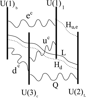
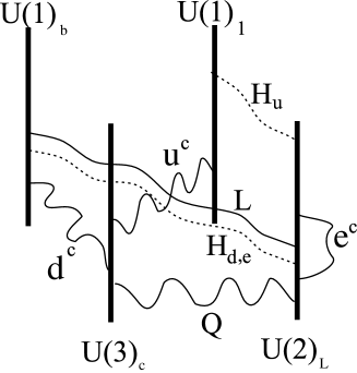
Figure 1: Pictorial representation of models $A,A^{\prime}$.

Apart from the hypercharge combination (2.7) all remaining abelian factors are anomalous. Indeed, for every abelian generator $Q_{I},I=(c,L,1,b)$, we can calculate the mixed gauge anomaly $K_{IJ}\equiv{\rm Tr}Q_{I}T^{2}_{J}$ with $J=SU(3),SU(2),Y$, and gravitational anomaly $K_{I4}\equiv{\rm Tr}Q_{I}$ for both models $A$ and $A^{\prime}$:

$$K^{(A)}=\left(\matrix{0&-1&-\frac{1}{2}&-\frac{1}{2}\cr\frac{3}{2}&-1&0&-\frac{1}{2}\cr-\frac{3}{2}&\frac{1}{3}&-\frac{1}{3}&\frac{1}{6}\cr 0&-4&-2&-4}\right)\ ,\ K^{(A^{\prime})}=\left(\matrix{0&-1&-\frac{1}{2}&-\frac{1}{2}\cr\frac{3}{2}&-1&0&-\frac{1}{2}\cr-\frac{3}{2}&-\frac{5}{3}&-\frac{4}{3}&-\frac{5}{6}\cr 0&-6&-3&-5}\right)$$ (2.8)

It is easy to check that the matrices $KK^{T}$ for both models have only one zero eigenvalue corresponding to the hypercharge combination (2.7) and three non vanishing ones corresponding to the orthogonal $U(1)$ anomalous combinations. In the context of type I string theory, these anomalies are canceled by a generalized Green-Schwarz mechanism which makes use of three axions that are shifted under the corresponding $U(1)$ anomalous gauge transformations. As a result, the three extra gauge bosons become massive, leaving behind the corresponding global symmetries unbroken in perturbation theory [49]. The three extra $U(1)$’s can be expressed in terms of known SM symmetries:

$$\mbox{Baryon number}\,\ \ \ B = \frac{1}{3}Q_{c}$$

$$\mbox{Lepton number}\,\,\ \ \ L = \frac{1}{2}\left(Q_{c}+Q_{L}-Q_{1}-Q_{b}\right)$$ (2.9)

$$\mbox{Peccei--Quinn}\ \ \ Q_{PQ} = -\frac{1}{2}\left(Q_{c}-Q_{L}-3\,Q_{1}-3\,Q_{b}\right)$$

Thus, our effective SM inherits baryon and lepton number as well as Peccei–Quinn (PQ) global symmetries from the anomaly cancellation mechanism. Note however that $PQ$ is the original Peccei–Quinn symmetry only in model $A^{\prime}$, such that all fermions have charges $+1$, while $H_{u}$ and $H_{d}$ have charges $-2$ and $+2$, respectively. In model $A$, the global $PQ$ symmetry defined in (2.9) is similar but with lepton charge +3. The reason is that in model $A$ the fermion-Higgs Yukawa couplings are different, and leptons get masses from $H_{u}$ and not from $H_{d}$.

The general one-loop string computation of the masses of anomalous $U(1)$ gauge bosons, as well as their localization properties in the internal compactified space, was performed recently for generic orientifold vacua [23]. It was shown that orbifold sectors preserving $N=1$ supersymmetry yield four-dimensional (4d) contributions, localized in the whole six-dimensional (6d) internal space, while $N=2$ supersymmetric sectors give 6d contributions localized only in four internal dimensions. The latter are related to 6d anomalies. Thus, even $U(1)$s which are apparently anomaly free may acquire non-zero masses at the one-loop level, as a consequence of 6d anomalies. These results have the following implications in our case:

1. The two $U(1)$ combinations, orthogonal to the hypercharge and localized on the strong and weak D-brane sets, acquire in general masses of the order of the string scale from contributions of $N=1$ sectors, in agreement with effective field theory expectations based on 4d anomalies.

2. Such contributions are not sufficient though to make heavy the third $U(1)$ propagating in the bulk, since the resulting mass terms are localized and suppressed by the volume of the bulk. In order to give string scale mass, one needs instead $N=2$ contributions associated to 6d anomalies along the two large bulk directions.

3. Special care is needed to guarantee that the hypercharge remains massless despite the fact that it is anomaly free.

The presence of massive gauge bosons associated to anomalous abelian gauge symmetries is generic. Their mass is given by $M_{A}^{2}\sim g_{s}M_{s}^{2}$, up to a numerical model dependent factor and is typically smaller by a factor or 2-5 than the string scale. When the latter is low, they can affect low energy measurable data, such as $g-2$ for leptons [35] and the $\rho$-parameter [32], leading to additional bounds on the string scale.

An extension of the model is the introduction of a right-handed neutrino in the bulk. A natural candidate state would be an open string ending on the ${U(1)}_{b}$ brane. Its charge is then fixed to $+2$ by the requirement of existence of the single possible neutrino mass term $L\,H_{d}\,\nu_{R}$. The suppression of the brane-bulk couplings due to the wave function of $\nu_{R}$ would thus provide a natural explanation for the smallness of neutrino masses. Note that if the zero mode of this bulk neutrino state is chiral, the anomaly structure of the model changes: $B-L$ becomes anomaly free and as a consequence the associated gauge boson remains in principle massless. However, as we discussed above, this is not in general true because of 6d anomalies [23]. In any case, this problem is absent if we introduce a vector-like bulk neutrino pair

$${\nu}_{R}(\textbf{1},\textbf{1},0,0,0,+2)+{\nu}^{c}_{R}(\textbf{1},\textbf{1},0,0,0,-2)$$

that leaves the anomalies (2.8) intact. Note that ${\nu}^{c}_{R}$ does not play any role in the subsequent discussion of neutrino masses and oscillations.

Models mLSOM_B and mLSOM${}_{B}^{\prime}$

Another phenomenologically promising pair of models consists of two models, named hereafter $B$ and $B^{\prime}$, which correspond to the hypercharge embedding

$$Y=\frac{2}{3}\,Q_{c}-\frac{1}{2}\,Q_{L}+Q_{1}\,.$$ (2.10)

The spectrum is

$$Q(\textbf{3},\textbf{2},+1,+1,0,0)$$

$$u^{c}(\bar{\textbf{3}},\textbf{1},-1,0,0,1)$$

$$d^{c}(\bar{\textbf{3}},\textbf{1},-1,0,1,0)$$

$$L(\textbf{1},\textbf{2},0,+1,0,-1)$$

$$e^{c}(\textbf{1},\textbf{1},0,0,+1,+1)$$

$$H_{u}(\textbf{1},\textbf{2},0,-1,0,-1)$$

$$H_{d}(\textbf{1},\textbf{2},0,+1,+1,0)$$

for model $B$, while in $B^{\prime}$ $e^{c}$ is replaced by $e^{c}(\textbf{1},\textbf{1},0,-2,0,0)$.

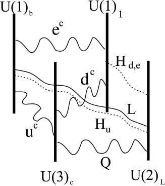
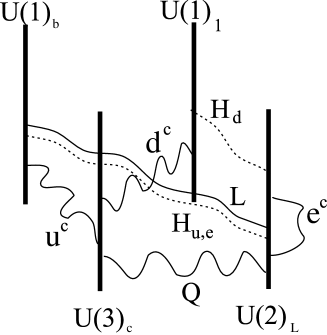
Figure 2: Pictorial representation of models $B$ and $B^{\prime}$.

The four abelian gauge factors are anomalous. Proceeding as in the analysis (2.8) of models $A$ and $A^{\prime}$, the mixed gauge and gravitational anomalies are

$$K^{(B)}=\left(\matrix{0&1&\frac{1}{2}&\frac{1}{2}\cr\frac{3}{2}&2&0&-\frac{1}{2}\cr-\frac{3}{2}&\frac{2}{3}&\frac{4}{3}&\frac{11}{6}\cr 0&8&4&2}\right)\ ,\ K^{(B^{\prime})}=\left(\matrix{0&1&\frac{1}{2}&\frac{1}{2}\cr\frac{3}{2}&2&0&-\frac{1}{2}\cr-\frac{3}{2}&-\frac{4}{3}&\frac{1}{3}&\frac{5}{6}\cr 0&6&3&1}\right)$$ (2.11)

It is easy to see that the only anomaly free combination is the hypercharge (2.10) which survives at low energies. All other abelian gauge factors are anomalous and will be broken by the generalized Green-Schwarz anomaly cancelation mechanism, leaving behind global symmetries. They can be expressed in terms of the usual SM global symmetries as the following ${U(1)}$ combinations:

$$\mbox{Baryon number}\,\ \ \ B = \frac{1}{3}\,Q_{c}$$ (2.12)

$$\mbox{Lepton number}\ \ \ \ L = -\frac{1}{2}\left(Q_{c}-Q_{L}+Q_{1}+Q_{b}\right)$$ (2.13)

$$\mbox{Peccei-Quinn}\ \ \ Q_{PQ} = \frac{1}{2}\left(-Q_{c}+3\,Q_{L}+Q_{1}+Q_{b}\right)$$ (2.14)

Similarly to the analysis of models $A$ and $A^{\prime}$, the $PQ$ charges defined above are the traditional ones only for model $B$. In model $B^{\prime}$, the lepton charge is $-3$, as a result of the Higgs Yukawa couplings to the fermions (see below). The right handed neutrino can also be accommodated as an open string with both ends on the bulk abelian brane:

$${\nu_{R}}(\textbf{1},\textbf{1},0,0,0,+2)+{\nu^{c}_{R}}(\textbf{1},\textbf{1},0,0,0,-2)$$

3 The effective action of the mLSOM

We will consider models which can originate from a non-supersymmetric string compactification where the Standard Model is localized on D-branes and/or intersections of D-branes in the presence of orientifold planes. The low energy limit of such models, assuming that they contain the Standard Model spectrum, is marked by the presence of extra $U(1)$ gauge bosons and of a certain number of scalar fields with axion and Stückelberg couplings. Consistency of these models and more specifically the cancellation of anomalies requires also certain Chern-Simons type of couplings.

Therefore apart from the Standard model fields, we have three more U(1)’s, three scalars (axions) that mix with the U(1)’s, and two Higgs doublets.

The minimal Lagrangian consistent with these features is

$${\cal L}\;= - \frac{1}{2}tr\;G_{\mu\nu}G^{\mu\nu}-\frac{1}{2}tr\;W_{\mu\nu}W^{\mu\nu}-\frac{1}{4}F_{\mu\nu}^{l}F^{\mu\nu,{l}}$$ (3.1)

$$- |(\partial_{\mu}+i\frac{g_{2}}{2}{\tau^{a}}W_{\mu}^{a}+iq_{l}^{(H_{u})}g_{l}A_{\mu}^{l})H_{u}|^{2}-|(\partial_{\mu}+i\frac{g_{2}}{2}{\tau^{a}}W_{\mu}^{a}+iq_{l}^{(H_{d})}g_{l}A_{\mu}^{l})H_{d}|^{2}$$

$$+ Q^{{\dagger}}_{Li}\sigma^{\mu}{\cal D}_{\mu}Q_{Li}+{u}^{{\dagger}}_{Ri}{\overline{\sigma}}^{\mu}{\cal D}_{\mu}{u}_{Ri}+{d}^{{\dagger}}_{Ri}{\overline{\sigma}}^{\mu}{\cal D}_{\mu}{d}_{Ri}$$

$$+ L^{{\dagger}}_{Li}\sigma^{\mu}{\cal D}_{\mu}L_{Li}+{e}^{{\dagger}}_{Ri}{\overline{\sigma}}^{\mu}{\cal D}_{\mu}{e}_{Ri}+{\nu}^{{\dagger}}_{Ri}{\overline{\sigma}}^{\mu}{\cal D}_{\mu}{\nu}_{Ri}$$

$$+ \gamma^{u}_{ij}H^{T}_{u}\tau^{2}\;(Q_{Li}^{t}\sigma^{2}u_{Rj})+\gamma^{d}_{ij}H^{{\dagger}}_{d}\;(Q_{Li}^{t}\sigma^{2}d_{Rj})+c.c.$$

$$+ \gamma^{e}_{ij}H^{{\dagger}}_{u}\;(L_{Li}^{t}\sigma^{2}e_{Rj})+\gamma^{\nu}_{ij}H^{T}_{d}\tau^{2}\;(L_{Li}^{t}\sigma^{2}{\nu}_{Rj})+c.c.$$

$$- \frac{1}{2}\sum_{I}(\partial_{\mu}a^{I}+g_{l}{\cal M}^{I}_{l}A^{l}_{\mu})^{2}+{E}_{lmn}\;\epsilon^{\mu\nu\rho\sigma}\;{A}^{l}_{\mu}\,{A}^{m}_{\nu}\,F^{n}_{\rho\sigma}$$

$$+ \sum_{I}({D}_{I}\,{a}^{I}\;tr\,\{G\wedge{G}\}+{F}_{I}\,{a}^{I}\;tr\,\{W\wedge{W}\}+{C}_{Imn}\,{a}^{I}\,F^{m}\wedge{F}^{n})$$

$$+ V(H_{u},H_{d},a^{I}).$$

where we have introduced two dimensional notations for the fermion interactions, as specified below. The gauge symmetry under which this Lagrangian is invariant is

$$SU(3)_{c}\times SU(2)_{W}\times G_{1},\hskip 28.45274ptG_{1}=\prod_{l=1}^{4}U(1)_{l}.$$ (3.2)

The $U(1)$ factors are all anomalous in general. In the above the indices $l,m,n=1,\cdots,4$ count the $U(1)$s in the D-brane basis. There is also a sum over $SU(2)$ indices $a=1,2,3$ and a sum over flavor indices $i=1,2,3$. $G_{\mu\nu}$ is the field strength for the gluons and the $W_{\mu\nu}$ is the field strength of the weak gauge bosons $W_{\mu}$. The fermions in eq. (3.1) are either left handed Weyl spinors $f_{L}$, or right handed Weyl spinors $f_{R}$ and they fall in the usual $SU(3)$ and $SU(2)$ representations of the Standard Model. The covariant derivatives act on the fermions $f_{L},f_{R}$ as

$${\cal D}_{\mu}f_{L}=\left(\partial_{\mu}+i{\bf A}_{\mu}+iq_{l}^{(f_{L})}g_{l}A_{l,\mu}\right)f_{L}$$

$${\cal D}_{\mu}f_{R}=\left(\partial_{\mu}+i{\bf A}_{\mu}-iq_{l}^{(f_{R})}g_{l}A_{l,\mu}\right)f_{R}$$ (3.3)

where ${\bf A}_{\mu}$ is a non abelian Lie algebra element. The matrices $\sigma^{\mu}=(\sigma^{0},\sigma^{a})$ where $\sigma^{0}=diag(1,1)$, $\sigma^{a}$ are the Pauli matrices and ${\overline{\sigma}}^{\mu}=(\sigma^{0},-\sigma^{a})$. We have also introduced two Higgs $SU(2)$ doublets $H_{u}$ and $H_{d}$. The matrices $\tau^{j}$ are Pauli matrices acting on $SU(2)$ indices.

In the Yukawa sector, the Pauli matrix $\tau^{2}$ acts on the $SU(2)$ indices while the Pauli matrix $\sigma^{2}$ acts on the spinor indices. The symbol $T$ ($t$) suggests transposition with respect to $SU(2)$ (spinor) indices. To lighten the notation we do not show explicitly the $SU(3)$ contraction. It should be understood however that the quarks are, on the top of all contractions explicitly shown, contracted as ${\bf q_{L}}^{\dagger}{\bf q_{R}}$ in the $SU(3)$ sense. The $\gamma^{u}_{ij}$ etc. are complex three by three matrices. The standard procedure is to bring them in a form as close as possible to diagonal. The result of this is

$${\cal L}_{\rm Yuk.} = \sum_{i,j}H^{T}_{u}\tau^{2}\;(Q_{Li}^{t}\sigma^{2}{\cal U}^{q}_{ji}\Gamma^{u}_{jj}u_{Rj})+\sum_{i}H^{{\dagger}}_{d}\;(Q_{Li}^{t}\sigma^{2}\Gamma^{d}_{ii}d_{Ri})+c.c.$$ (3.4)

$$+ \sum_{i,j}H^{{\dagger}}_{u}\;(L_{Li}^{t}\sigma^{2}{\cal U}^{\nu}_{ji}\Gamma^{e}_{jj}e_{Rj})+\sum_{i}H^{T}_{d}\tau^{2}\;(L_{Li}^{t}\sigma^{2}{\Gamma^{\nu}_{ii}\nu}_{Ri})+c.c.$$

where the $\Gamma^{u,d,e,\nu}$ are diagonal matrices and ${\cal U}^{q}$ is the CKM matrix which appears in the Yukawa sector of this model in a similar way as in the Standard Model. The ${\cal U}^{\nu}$ matrix is the MNS neutrino mixing matrix. In the electroweak vacuum the Higgs couples universally to the Yukawa sector and the Yukawa couplings turn into mass terms for the fermions. The CKM and MNS matrices disappear from the Yukawa couplings but they appear explicitly in the gauge boson-fermion-fermion interactions, as we will see later. Issues of flavor in intersecting D-brane models are discussed in [53, 54, 55] and references therein.

The couplings ${\cal M}^{I}_{m}$, $F_{I}$, $D_{I}$, $C_{Imn}$ and $E_{lmn}$ are known once a specific string vacuum has been chosen. One feature of the action, as we are going to describe below, is the presence of both dimension-4 and dimension-5 operators, which render it an effective non-renormalizable extension of the Standard Model. The mechanism of cancellation of the anomalies which is enforced on the model is different from the Standard Model one and for this reason all the couplings the $E$, $D$, and $C$ carry an intrinsic power of $h$, the Planck constant, in their definition. The index $I=1,\cdots,N_{a}$ runs over the scalars with axion couplings whose number is in general different (and usually much larger) than the number of $U(1)$ fields. In the mLSOM the number of relevant axions will be taken to be always one less than the number of $U(1)$s (i.e. the number of D-brane stacks), in our case $N_{a}=3$.

Finally, the Higgs potential is one that is consistent with the symmetries of the theory and breaks the electroweak symmetry spontaneously down to electromagnetism as in the SM. In general it can depend on all scalar fields present in the spectrum, namely both on the Higgs fields and on the axions, provided it is compatible with the gauge invariances. We will split the Higgs potential in two parts. The one in eq. (4.1) which does not depend on the axions, and the one in eq. (LABEL:PQbreak) which mixes the Higgs doublets with the pseudo-scalars.

3.1 Changing basis in gauge symmetry space.

A first interesting aspect of such models is that some of the the gauge bosons can pick up masses even in the absence of electroweak (EW) symmetry breaking because of (potential) anomalies. Indeed, by inspecting eq. (3.1) one can see that there are couplings that give a tree-level mass to the anomalous $U(1)$ gauge bosons without a Higgs mechanism. The mass squared matrix of the 4 $U(1)$ gauge bosons is

$${\bf M}={\cal M}^{T}{\cal M}$$ (3.5)

which in general is a real, symmetric but non-diagonal matrix. The dimension of ${\bf M}$ is equal to the number of $U(1)$s. In order to simplify the expressions as much as possible, we absorb in its elements the corresponding factors of the gauge couplings. ${\bf M}$ is real and symmetric thus it can be diagonalized by an orthogonal transformation

$${\bf M}=O^{T}{\bf m}\;O$$ (3.6)

where $O$ is the appropriate orthogonal matrix. The diagonal matrix ${\bf m}$ contains the eigenvalues of ${\bf M}$, i.e. the masses squared of the gauge bosons. When $N_{a}=N_{s}-1$, where $N_{s}$ is the number of stacks, ${\bf m}$ contains at least one zero eigenvalue.

To write the other terms in the action in the new basis, we start from the $U(1)$ sector in the D-brane basis and focus for the moment on the gauge kinetic and the gauge-fermion-fermion interaction terms

$$\sum_{l}{1\over 4\tilde{g}_{l}^{2}}{F_{l}}^{2}+\sum_{l}A_{l}\,\bar{\psi}\,q_{l}\,\psi,$$ (3.7)

where the charges are normalized to integers and

$$\tilde{g}_{l}={g_{l}\over\sqrt{2N}},$$ (3.8)

where $g_{l}$ is the standard normalized coupling of the associated SU(N) group.

We will keep three bulk axions, the number that is relevant to cancel the anomalies of the three anomalous U(1)’s.

The (normalized) hypercharge generator can be written as

$$q_{Y}=\sum_{l}k_{l}q_{l}.$$ (3.9)

We will rescale the gauge fields as $A_{l}\to\tilde{g}_{l}A_{a}$ to obtain

$$\sum_{l}{1\over 4}F_{l}^{2}+\sum_{l}\tilde{g}_{l}~{}A_{l}\bar{\psi}\,q_{l}\,\psi.$$ (3.10)

We will now do an orthogonal transformation to go to a basis where one of the gauge fields is the hypercharge while the rest have a diagonal UV mass matrix

$$A_{l}=\sum_{l^{\prime}}O_{ll^{\prime}}A^{l^{\prime}},\;\;,\;\;OO^{T}=1.$$ (3.11)

The index $l^{\prime}$ in the new basis (referred to as the hypercharge basis from now on) runs through $l^{\prime}=Y,I$, with $I$ running through the last $3$ values. For the above transformation to be consistent, we must take

$$\tilde{g}_{l}\,O_{l{Y}}\sim k_{l}~{}~{}~{}\forall l.$$ (3.12)

Normalizing we obtain

$$O_{lY}=g_{Y}{k_{l}\over\tilde{g}_{l}}\;\;,\;\;{1\over g_{Y}^{2}}=\sum_{l}{k_{l}^{2}\over\tilde{g}_{l}^{2}}.$$ (3.13)

We must now pick the $3$ vectors $\vec{n}_{I}=O_{iI}$ so that they are orthogonal to the hypercharge, they are normalized, and they diagonalize the mass matrix. They can be parameterized in terms of 3 SO(3) angles but we will keep it as such for the moment. The transformation of any of the charges is

$$q_{l^{\prime}}=\sum_{l}q_{l}\frac{{\tilde{g}}_{l}}{g_{l^{\prime}}}O_{{l}l^{\prime}}\equiv\sum_{l}q_{l}U_{{l}^{\prime}l}.$$ (3.14)

We can then use the matrix $U$ defined by the second part of the above equation to express the couplings in the new basis in terms of the couplings in the old basis:

$$\frac{\delta_{{l}^{\prime}{m^{\prime}}}}{g_{l^{\prime}}{g_{m^{\prime}}}}=\sum_{l}\frac{U_{{l}^{\prime}l}U_{{m}^{\prime}l}}{{\tilde{g}}_{l}^{2}}.$$ (3.15)

Next, we must rotate the Green-Schwarz couplings. As we will show, in this basis the Stückelberg couplings take the simple form

$$\frac{1}{2}\sum_{I}(\partial a_{I}^{\prime}+M_{I}A^{I})^{2}$$ (3.16)

with $a_{I}^{\prime}$ the hypercharge basis axions and $M_{I}$ the (square root of the) non-zero eigenvalues contained in ${\bf m}$.

3.2 Anomalous couplings

This section is devoted to the discussion of the terms in eq. (3.1) referred to as Green-Schwarz couplings. It should be clear by now that the low energy effective action that corresponds to low scale orientifold vacua has certain distinctive features. To begin, most of the extensions of the Standard Model that are widely believed to be experimentally testable, such as the MSSM or the NMSSM, are essentially usual gauge theories coupled in a conventional way to a larger set of matter fields than the one encountered in the SM. By this we mean that all the couplings that one finds in these extensions are of the same type as the couplings of the SM. The reason for qualitatively new types of couplings not being necessary in these conventional models is the way gauge anomalies cancel. In the MSSM for example, anomalies cancel in the same way as in the SM: the anomaly of each gauge factor vanishes separately. In string theory, however, there is room for an alternative way to cancel anomalies, via the Green-Schwarz mechanism.

The net effect of the Green-Schwarz mechanism on the four-dimensional effective action is a number of scalar fields with Stückelberg and axion-like couplings and certain Chern-Simons couplings. It is also interesting to point out that these unusual couplings are remnants of the interplay between closed and open strings from the string theory point of view or the gravitational and gauge sectors in the language of the low energy effective action. The pseudoscalar axions originate from (closed string sector) RR fields coupled to the (open string sector) gauge fields of the D-brane world volume through the Wess-Zumino effective action. Besides their theoretical interest, the presence of these terms may provide us with a unique opportunity to test string theory experimentally.

The D-brane basis Stückelberg couplings in eq. (3.1) can be then written in matrix form as

$${\cal L}^{Stuck}=\frac{1}{2}\sum_{I}(\partial_{\mu}\,{a}^{I}+{\cal M}^{I}_{l}{A}_{\mu}^{l})(\partial_{\mu}\,{a}^{I}+{\cal M}^{I}_{l}{A}_{\mu}^{l})$$ (3.17)

and as we have seen in detail, ensure that some of the $U(1)$s pick up masses of the order of the string scale.

The other Green-Schwarz couplings in eq. (3.1) consist of the axion-like terms

$${\cal L}^{axion}={D}_{I}\,{a}^{I}\;tr\,\{G\wedge{G}\}+{F}_{I}\,{a}^{I}\;tr\,\{W\wedge{W}\}+{C}_{Imn}\,{a}^{I}\,F^{m}\wedge{F}^{n}$$ (3.18)

where we have introduced the dimensionfull couplings ${D}_{I}$, ${F}_{I}$ and ${C}_{Imn}$ and the Chern-Simons terms [28],

$${\cal L}^{C-S}={E}_{lmn}\;\epsilon^{\mu\nu\rho\sigma}\;{A}^{l}_{\mu}{A}^{m}_{\nu}F^{n}_{\rho\sigma}.$$ (3.19)

In the above the sum over $l,m,n$ is implied. Under the $U(1)$ gauge transformation

$${A}_{\mu}^{l}\longrightarrow{A}_{\mu}^{l}+\partial_{\mu}{\epsilon}^{l}$$ (3.20)

with ${\bf\epsilon}$ the gauge transformation parameters, the anomalous variation of the Lagrangian is

$${{\cal L}^{1-loop}=\bf\epsilon}^{l}\left[g_{l}g_{3}^{2}\,\Lambda_{3}\,{t}^{(3)}_{l}\,G\wedge{G}+g_{l}g_{2}^{2}\,\Lambda_{2}\,{t}^{(2)}_{l}\,W\wedge{W}+\Lambda_{1}\,g_{l}g_{m}g_{n}\,{t}^{(1)}_{lmn}\,F^{m}\wedge{F}^{n}\right]$$ (3.21)

where

$$t^{(1)}_{lmn}=tr(q_{l}q_{m}q_{n}),\hskip 14.22636ptt^{(1)}_{llm}=\frac{1}{2!}tr(q_{l}^{2}q_{m}),\hskip 14.22636ptt^{(1)}_{lll}=\frac{1}{3!}tr(q_{l}^{3})$$ (3.22)

and

$$t^{(3)}_{l}=tr(q_{l}T^{A}T^{A}),\hskip 28.45274ptt^{(2)}_{l}=tr(q_{l}T^{j}T^{j}).$$ (3.23)

Here the index $A$ ($a$) labels the generators of $SU(3)$ ($SU(2)$). The nature and meaning of the quantities $\Lambda_{1}$, $\Lambda_{2}$ and $\Lambda_{3}$ is clear once the anomaly diagrams are explicitly computed in momentum space. They can be seen to be the shift necessary to be performed in the momentum integration of the triangle anomaly diagram so that the Green-Schwarz anomaly cancellation mechanism is reflected by the Ward identities.

The axions transform under the $U(1)$ transformations as

$${a}^{I}\longrightarrow{a}^{I}-{\cal M}^{I}_{l}\,{\epsilon^{l}}.$$ (3.24)

The Stückelberg and the axion-gauge-gauge couplings are gauge invariant separately but the Chern-Simons term is not. The gauge variation of the latter is cancelled by the anomaly. By comparing the different gauge variations, we can easily read off the four dimensional version of the Green-Schwarz anomaly cancellation conditions

$${D}_{I}\;{\cal M}^{I}_{l}=\Lambda_{3}\;g_{l}g_{3}^{2}\,t_{l}^{(3)}$$ (3.25)

$${F}_{I}\;{\cal M}^{I}_{l}=\Lambda_{2}\;g_{l}g_{2}^{2}\,t_{l}^{(2)}$$ (3.26)

$${C}_{Imn}\;{\cal M}^{I}_{l}+(E_{lmn}-E_{mln})=\Lambda_{1}\,g_{l}g_{m}g_{n}\,t^{(1)}_{lmn}.$$ (3.27)

The first two of the above, eqs. (3.25) and (3.26) represent the cancellation of the anomalous triangle graph with a $U(1)_{l}$ gauge boson and two gluons and $SU(2)$ gauge bosons for external legs respectively. The third, eq. (3.27) represents the mixed $U(1)$ anomaly cancellation.

We can put some restrictions on the couplings $E_{lmn}$. Define

$$S^{lmn}\equiv\int\epsilon^{\mu\nu\rho\sigma}A_{\mu}^{l}A_{\nu}^{m}F_{\rho\sigma}^{n}$$ (3.28)

which transforms as

$$\delta S^{lmn}=\int(-\epsilon^{l}F^{m}\wedge F^{n}+\epsilon^{m}F^{l}\wedge F^{n}).$$ (3.29)

It is easy to see that $S^{lmn}$ satisfy

$$S^{mln}=-S^{lmn}$$ (3.30)

and that the transformation property of the Chern-Simons couplings is

$$\delta(E_{lmn}S^{lmn})=\int(E_{mln}-E_{lmn})\epsilon^{l}F^{m}\wedge F^{n},$$ (3.31)

which was used to derive eq. (3.27). An immediate consequence of eq. (3.30) is that $E_{lmn}S^{lmn}$ vanishes identically unless $E_{lmn}$ is antisymmetric in the first two indices. Now, if $E_{lmn}$ is totally antisymmetric, then $E_{lmn}S^{lmn}$ can be seen to be again identically zero by using the identity

$$S^{lmn}+S^{nlm}+S^{mnl}=0$$ (3.32)

which can be derived by integrating by parts. Therefore the only choice left is the one where $E_{lmn}$ is antisymmetric in $lm$. Then, eq. (3.27) reduces to

$${C}_{Imn}\;{\cal M}^{I}_{l}+2E_{lmn}=\Lambda_{1}\,g_{l}g_{m}g_{n}\,t^{(1)}_{lmn}$$ (3.33)

and the gauge transformation to

$$\delta(E_{lmn}S^{lmn})=-2\,\int E_{lmn}\epsilon^{l}F^{m}\wedge F^{n}.$$ (3.34)

The rotation to the hypercharge basis can be done by means of eq. (3.6). The transformation of the vectors and axions consistent with eq. (3.6) is

$${A}_{l}\;=\;O_{l^{\prime}l}\,{A}_{l^{\prime}},\hskip 28.45274pt{a}^{I}\;=\;\sum_{J}{\cal M}^{I}_{l}\,O_{Jl}\,\frac{a^{\prime}_{J}}{M_{J}}$$ (3.35)

respectively, with $M_{J}$ the mass of the $J$ th gauge boson in the hypercharge basis. The sum over $l$ and $l^{\prime}$ is implicit but we show the sum over the indices $I$ explicitly when present. The proper gauge transformation rules become

$${A}_{l^{\prime}}\longrightarrow{A}_{l^{\prime}}+\partial\;{\epsilon^{\prime}}_{l^{\prime}}$$ (3.36)

$${a}_{I}^{\prime}\longrightarrow{a}_{I}^{\prime}-{M_{I}}\,{\bf\epsilon}^{\prime}_{I}$$ (3.37)

where $\epsilon^{\prime}=O\epsilon$ and the Stückelberg coupling transforms into

$${\cal L}^{Stuck}=\frac{1}{2}\sum_{I}(\partial_{\mu}{a}^{\prime}_{I}+M_{I}{A}^{I}_{\mu})^{2}.$$ (3.38)

Indeed, eq. (3.38) is precisely eq. (3.16), as claimed.

The Green-Schwarz couplings eqs. (3.18) and (3.19) can be written in the hypercharge basis as

$${\cal L}^{GS} = \sum_{I}({D^{\prime}_{I}}\,{a^{\prime}_{I}}\,tr\,\{G\wedge{G}\}+{F^{\prime}_{I}}\,{a^{\prime}_{I}}\,tr\,\{W\wedge{W}\}+{C^{\prime}}_{Im^{\prime}n^{\prime}}\,{a^{\prime}_{I}}\,F^{m^{\prime}}\wedge{F}^{n^{\prime}})$$

$$+ E_{l^{\prime}m^{\prime}n^{\prime}}\,\epsilon^{\mu\nu\rho\sigma}\,{A}^{l^{\prime}}_{\mu}{A}^{m^{\prime}}_{\nu}{F}^{n^{\prime}}_{\rho\sigma}$$

with

$${D^{\prime}_{I}}=\sum_{J}\frac{1}{M_{I}}{D}_{J}{\cal M}^{J}_{l}O_{Il},\hskip 28.45274pt{F^{\prime}_{I}}=\sum_{J}\frac{1}{M_{I}}{F}_{J}{\cal M}^{J}_{l}O_{Il},$$

$${C^{\prime}_{I}}_{m^{\prime}n^{\prime}}=\sum_{J}\frac{1}{M_{I}}{C}_{Jmn}{\cal M}^{J}_{l}O_{Il}O_{m^{\prime}n}O_{n^{\prime}n}$$ (3.40)

and

$$E_{l^{\prime}m^{\prime}n^{\prime}}=E_{lmn}O_{l^{\prime}l}O_{m^{\prime}m}O_{n^{\prime}n}.$$ (3.41)

It is now straightforward to show that the Green-Schwarz anomaly cancellation conditions in the hypercharge basis are

$${D}^{\prime}_{I}\;{M_{I}}=\Lambda_{3}\,g_{I}^{2}g_{3}\,{t^{\prime}}^{(3)}_{I}$$ (3.42)

$${F}^{\prime}_{I}\;{M_{I}}=\Lambda_{2}\,g_{I}^{2}g_{2}\,{t^{\prime}}^{(2)}_{I}$$ (3.43)

$${C}^{\prime}_{Im^{\prime}n^{\prime}}\;{M_{I}}+2E_{Im^{\prime}n^{\prime}}=\Lambda_{1}\,g_{I}g_{m^{\prime}}g_{n^{\prime}}\,{t^{\prime}}^{(1)}_{Im^{\prime}n^{\prime}}$$ (3.44)

with the anomaly coefficients ${t^{\prime}}^{(1,2,3)}$ computed in the hypercharge basis.

3.3 Gauge fixing in the unbroken phase

We work in the $(Y,I)$ basis, with $Y$ the hypercharge and $I$ the index denoting the anomalous $U(1)$ gauge bosons in the hypercharge basis.

A useful gauge is the one where the axions become longitudinal components of the massive anomalous gauge fields. Clearly, in this gauge there should be no direct axion-gauge boson interactions. It is not hard to come up with a gauge where the unphysical couplings of the type

$$M_{I}\;(\partial\cdot A_{I})\;a_{I}^{\prime}$$ (3.45)

are absent. The necessary gauge fixing functions for $SU(3)$, $SU(2)$, $U(1)_{Y}$ and the $U(1)_{I}$ are

$${\cal G}^{A}=\partial\cdot G^{A}$$ (3.46)

$${\cal G}^{a}=\partial\cdot W^{a}$$ (3.47)

$${\cal G}^{Y}=\partial\cdot A^{Y}$$ (3.48)

$${\cal G}^{I}=\partial\cdot A^{I}+\alpha_{I}M_{I}\;a_{I}^{\prime}$$ (3.49)

respectively, where we have introduced gauge fixing functions with real parameters $\alpha_{I}$ for the anomalous $U(1)$s. The gauge fixing terms are

$${\cal L}^{gf}=\frac{1}{2\alpha_{3}}{\cal G}^{A}{\cal G}^{A}+\frac{1}{2\alpha_{2}}{\cal G}^{a}{\cal G}^{a}+\frac{1}{2\alpha_{Y}}{{\cal G}^{Y}}{{\cal G}^{Y}}+\sum_{I}{\cal L}_{gf}^{I},\hskip 14.22636pt{\cal L}_{gf}^{I}=\frac{1}{2\alpha_{I}}{{\cal G}^{I}}{{\cal G}^{I}}$$ (3.50)

and the ghost terms are

$${\cal L}^{gh}=\eta^{*A}\frac{\delta{\cal G}^{A}}{\delta{w}^{B}}\eta^{B}+\eta^{*a}\frac{\delta{\cal G}^{a}}{\delta{w}^{b}}\eta^{b}+(\partial\eta^{*Y})\cdot(\partial\eta^{Y})+\sum_{I}{\cal L}_{gh}^{I},$$

where in the $SU(3)$ part

$$\frac{\delta{\cal G}^{A}}{\delta{w}^{B}}=-(\partial\cdot\partial)\,\delta^{AB}-f^{ABC}(\partial\cdot G^{C})$$ (3.52)

is the change of the gauge function under a gauge transformation parameterized by $\omega^{B}$ and $\eta^{*A}$ and $\eta^{A}$ are the anticommuting ghost fields. Analogous is the notation for the other gauge groups. We will now derive ${\cal L}_{\rm gh}^{I}$.

Under the gauge fixing conditions, the Stückelberg Lagrangian describing the dynamics of each anomalous gauge boson is given by

$${\cal L}_{Stueck}^{I}=-\frac{1}{4}F_{I\,\mu\nu}^{2}-\frac{1}{2}\left(\partial^{\mu}a_{I}^{\prime}+M_{I}A^{I}_{\mu}\right)^{2}+\frac{1}{2\alpha_{I}}\left(\partial_{\mu}A_{I}^{\mu}+\alpha_{I}\,M_{I}\,a_{I}^{\prime}\right)^{2}.$$ (3.53)

The action is not gauge invariant under the full $U(1)_{I}$ gauge transformation parameterized by $\epsilon_{I}^{\prime}$, it is however invariant under gauge transformations that satisfy

$$(\partial^{2}-\alpha_{I}M_{I}^{2})\;\epsilon_{I}^{\prime}=0.$$ (3.54)

One should now observe that these are just the equations of motion of the $a_{I}^{\prime}$ and therefore that gauge transformations performed by the axions playing the role of the gauge functions are a symmetry of the gauge fixed action. In fact, the model could be extended to include an anomalous fermion interaction of the form

$${\cal L}_{f}^{I}=\bar{\psi}\left[\left(g_{V}\gamma^{\mu}-g_{A}\gamma^{\mu}\gamma_{5}\right)\left(i\partial_{\mu}+g_{I}\,A^{I}_{\mu}\right)\right]\psi.$$ (3.55)

The total Lagrangian (barring ghosts) is then invariant under the transformations

$$\delta\,{A^{I}}_{\mu}=\partial_{\mu}a_{I}^{\prime}$$

$$\delta\,a_{I}^{\prime}=-M_{I}\,a_{I}^{\prime}$$

$$\psi\longrightarrow{\rm e}^{ig_{I}a_{I}^{\prime}}\psi$$

$${\bar{\psi}}\longrightarrow{\rm e}^{-ig_{I}a_{I}^{\prime}}\bar{\psi}.$$ (3.56)

Let us now derive the remnant symmetry when we include ghosts. If we denote by $\eta_{I}(x)$ and $\eta_{I}^{*}(x)$ independent anticommuting scalar fields, the Lagrangian is by construction invariant under the transformation ${\bf s}$:

$${\bf s}\,A^{I}_{\mu}=\partial_{\mu}\eta_{I}$$

$${\bf s}\,a_{I}^{\prime}=-M_{I}\,\eta_{I}$$

$${\bf s}\,\psi=i\,g_{I}\,\eta_{I}\;\psi$$

$${\bf s}\,\bar{\psi}=-i\,g_{I}\,\eta_{I}\;\bar{\psi}$$

$${\bf s}\,\eta_{I}=0$$ (3.57)

which can be read off eq. (3.56). The above BRST transformation is nilpotent even off shell (${\bf s}^{2}=0$) and $\eta_{I}$ are free, i.e. not constrained by the Klein-Gordon like equation eq. (3.54). In terms of the new fields the gauge fixing plus ghost Lagrangian in the quantum action is of the form

$${\cal L}_{\rm gh}^{I}+{\cal L}_{\rm gf}^{I}=-\eta_{I}^{*}({\bf s}\,{\cal G}_{I})+\frac{1}{2\alpha_{I}}{\cal G}_{I}^{2}$$ (3.58)

for a given gauge fixing function ${\cal G}_{I}$. We of course choose eq. (3.49) for the gauge fixing functions and for the ghost part we finally obtain the expression

$${\cal L}_{\rm gh}^{I}=-\eta_{I}^{*}\left(\partial^{2}-\alpha_{I}\,M_{I}^{2}\right)\eta_{I}.$$ (3.59)

4 Electroweak symmetry breaking

The electroweak symmetry breaking in mLSOM is a very interesting effect, because the Higgses are charged under the anomalous U(1) gauge symmetries.

In order to discuss EW symmetry breaking we have to be more specific about the Higgs potential. Before EW breaking the Abelian gauge symmetry in the $D$-brane basis is ${G}_{1}$ and the Higgs potential $V_{PQ}$ is the most general $SU(2)_{L}\times G_{1}$ invariant constructed from the two Higgs $SU(2)$ doublets $H_{u}$ and $H_{d}$:

$$V_{PQ}(H_{u},H_{d})=\sum_{a=u,d}\Bigl{(}\mu_{a}^{2}H_{a}^{\dagger}H_{a}+\lambda_{aa}(H_{a}^{\dagger}H_{a})^{2}\Bigr{)}-2\lambda_{ud}(H_{u}^{\dagger}H_{u})(H_{d}^{\dagger}H_{d})+2{\lambda^{\prime}_{ud}}|H_{u}^{T}\tau_{2}H_{d}|^{2}.$$ (4.1)

We can parameterize the Higgs fields in terms of 8 real degrees of freedom as

$$H_{u}=\left(\begin{array}[]{c}H_{u}^{+}\\ H_{u}^{0}\end{array}\right)\qquad H_{d}=\left(\begin{array}[]{c}H_{d}^{+}\\ H_{d}^{0}\end{array}\right)$$ (4.6)

where $H_{u}^{+}$, $H_{d}^{+}$ and $H_{u}^{0}$, $H_{d}^{0}$ are complex fields. Specifically

$$H_{u}^{+}=\frac{H_{uR}^{+}+iH_{uI}^{+}}{\sqrt{2}},\qquad H_{d}^{-}=\frac{H_{dR}^{-}+iH_{dI}^{-}}{\sqrt{2}},\qquad H_{u}^{-}=H_{u}^{+*},\qquad H_{d}^{+}=H_{d}^{-*}.$$ (4.7)

Expanding around the vacuum we get for the uncharged components

$$H_{u}^{0}=v_{u}+\frac{H_{uR}^{0}+iH_{uI}^{0}}{\sqrt{2}},\qquad H_{d}^{0}=v_{d}+\frac{H_{dR}^{0}+iH_{dI}^{0}}{\sqrt{2}}.$$ (4.8)

The Weinberg angle is defined via $\cos\theta_{W}=g_{2}/g,\sin\theta_{W}=g_{Y}/g$, with $g^{2}=g_{Y}^{2}+g_{2}^{2}$. We also define $\cos\beta=v_{d}/v$, $\sin\beta=v_{u}/v$ and $v^{2}=v_{d}^{2}+v_{u}^{2}$.

As in the MSSM one can set $H_{u}^{+}=0$ at the minimum by an $SU(2)$ transformation. Then a minimum with $\partial V/\partial H_{u}^{+}=0$ must also have $H_{d}^{+}=0$. A necessary condition for the potential $V_{PQ}$ to be bounded from below can be obtained by requiring that the potential is non-negative definite around the electroweak breaking vacuum:

$$\mu_{u}^{2}v_{u}^{2}+\mu_{d}^{2}v_{d}^{2}+\lambda_{uu}v_{u}^{4}+\lambda_{dd}v_{d}^{4}-2\lambda_{ud}v_{u}^{2}v_{d}^{2}\;\geq\;0.$$ (4.9)

The above constraint should be satisfied simultaneously with the constraint coming from the requirement that the vacuum $<H_{u}^{0}>\;=0$, $<H_{d}^{0}>\;=0$ (which does not trigger electroweak symmetry breaking) is an unstable minimum of the potential. This is the case when

$$\mu_{u}^{2}\mu_{d}^{2}\;\leq\;0.$$ (4.10)

Minimizing the potential with respect to $H_{u}^{0}$ and $H_{d}^{0}$ one can see that the Higgs vevs

$$H_{u}=v_{u}\pmatrix{0\cr 1},\hskip 56.9055ptH_{d}=v_{d}\pmatrix{0\cr 1}$$ (4.11)

do not break electric charge and minimize $V_{PQ}$ (at tree level) if

$$\pmatrix{\mu_{u}^{2}\cr\mu_{d}^{2}}=4\;\pmatrix{-\lambda_{uu}&\lambda_{ud}\cr\lambda_{ud}&-\lambda_{dd}}\pmatrix{v_{u}^{2}\cr v_{d}^{2}}$$ (4.12)

with $\lambda_{uu}$, $\lambda_{dd}$ and $\lambda_{ud}$ all real. Using the above conditions, the constraint eq. (4.9) becomes

$$\mu_{u}^{2}v_{u}^{2}+\mu_{d}^{2}v_{d}^{2}\;\geq\;0.$$ (4.13)

Furthermore, the couplings $\lambda_{uu}$, $\lambda_{dd}$ and $\lambda_{ud}$ should be such that eq. (4.10) and eq. (4.13) are also consistent.

4.1 The gauge boson masses

The vevs eq. (4.11), in addition to breaking $SU(2)_{L}\times{G^{\prime}_{1}}$ down to $U(1)_{\gamma}$, should not be in contradiction with the low energy EW data. The previous discussion for the gauge boson masses still applies with appropriate adjustments that take into account the effects of EW breaking. Technically speaking, the neutral $U(1)$ mass matrix ${\bf M}^{EW}$ should have precisely one zero eigenvalue consistent with an unbroken $U(1)_{\gamma}$.

${\bf M}^{EW}$ is the $5$ by $5$ matrix that can be read off the quadratic form

$$|{\cal D}_{\mu}H_{u}|^{2}+|{\cal D}_{\mu}H_{d}|^{2}+\frac{1}{2}\sum_{I}(\partial a_{I}^{\prime}+M_{I}A^{I})^{2}$$ (4.14)

and whose eigenvalues and eigenvectors we will now compute. Notice that as before, we have absorbed in $M_{I}$ a factor of $g_{I}$ in the Stückelberg part of the above formula. One can easily put it back in the following analysis by doing the rescaling $M_{I}\longrightarrow g_{I}M_{I}$. We will reinstate the couplings explicitly when we discuss NG bosons. The covariant derivatives are

$${\cal D}_{\mu}H_{u} = \left(\partial_{\mu}+\frac{i}{\sqrt{2}}g_{2}\left(T^{+}W^{+}+T^{-}W^{-}\right)+\frac{i}{2}g_{2}\tau_{3}W_{3\mu}+\frac{i}{2}g_{Y}A_{\mu}^{Y}+{i\over 2}\sum_{I}q^{I}_{u}g_{I}\,A^{I}_{\mu}\right)H_{u}$$

$${\cal D}_{\mu}H_{d} = \left(\partial_{\mu}+\frac{i}{\sqrt{2}}g_{2}\left(T^{+}W^{+}+T^{-}W^{-}\right)+i\frac{g_{2}}{2}\tau_{3}W_{3\mu}+\frac{i}{2}g_{Y}A_{\mu}^{Y}+{i\over 2}\sum_{I}q^{I}_{d}g_{I}\,A^{I}_{\mu}\right)H_{d}$$

where $q^{l}_{u,d}$ are the $U(1)$ charges of the two Higgses in the D-brane basis. They can be found for the four distinct configurations in section 2.1.

$$q_{u}^{I}\equiv\sum_{l}q^{l}_{u}\frac{\tilde{g}_{l}}{g_{I}}O_{iI},\hskip 28.45274ptq_{d}^{I}\equiv\sum_{l}q^{l}_{d}\frac{\tilde{g}_{l}}{g_{I}}O_{iI}$$ (4.15)

are the Higgs charges in the hypercharge basis. We have normalized the $U(1)$s so that

$$q_{u}^{Y}=q_{d}^{Y}=\frac{1}{2}.$$ (4.16)

The $SU(2)$ generators and gauge bosons are defined as

$$T^{j}=\frac{\tau^{j}}{2},\qquad T^{\pm}=T^{1}\pm iT^{2},\qquad W^{\pm}=\frac{1}{\sqrt{2}}\left(W^{1}\mp iW^{2}\right),$$ (4.17)

we obtain explicitly

$${\cal D}_{\mu}H_{u}=\pmatrix{\partial_{\mu}+\frac{i}{2}g_{2}W_{3\mu}+\frac{i}{2}{g_{Y}}A_{\mu}^{Y}+{i\over 2}\sum_{I}q^{I}_{u}g_{I}\,A^{I}_{\mu}&\frac{i}{\sqrt{2}}{g_{2}}{W^{+}}\cr\frac{i}{\sqrt{2}}{g_{2}}{W^{-}}&\partial_{\mu}-\frac{i}{2}g_{2}W_{3\mu}+\frac{i}{2}{g_{Y}}A_{\mu}^{Y}+{i\over 2}\sum_{I}q^{I}_{u}g_{I}\,A^{I}_{\mu}}H_{u}$$ (4.18)

and a similar expression for the covariant derivative of $H_{d}$. The mass matrix in the mixing of the neutral gauge bosons can be then computed from

$$\frac{1}{2}\sum_{I}M_{I}^{2}(A^{I}_{\mu})^{2}+{1\over 4}(-g_{2}W_{3\mu}+{g_{Y}}A_{\mu}^{Y}+\sum_{I}q^{I}_{u}\,g_{I}\,A^{I}_{\mu})^{2}v_{u}^{2}$$

$$+{1\over 4}(-g_{2}W_{3\mu}+{g_{Y}}A_{\mu}^{Y}+\sum_{I}q^{I}_{d}\,g_{I}\,A^{I}_{\mu})^{2}v_{d}^{2},$$ (4.19)

and it reads

$${\bf M}^{2}={1\over 4}\pmatrix{{g_{2}}^{2}v^{2}&-{g_{2}}{g_{Y}}v^{2}&-{g_{2}}x_{I}\cr-{g_{2}}{g_{Y}}v^{2}&{g_{Y}}^{2}v^{2}&{g_{Y}}x_{I}\cr-{g_{2}}x_{I}&{g_{Y}}x_{I}&2M_{I}^{2}\delta_{IJ}+N_{IJ}}$$ (4.20)

where

$$N_{IJ}=(q_{u}^{I}q_{u}^{J}v_{u}^{2}+q_{d}^{I}q_{d}^{J}v_{d}^{2})\,g_{I}g_{J}$$ (4.21)

$$x_{I}=(q_{u}^{I}v_{u}^{2}+q_{d}^{I}v_{d}^{2})\,g_{I}.$$ (4.22)

The zero eigenvalue corresponds to the photon

$$A_{\gamma}={g_{Y}\over{g}}W_{3}+{g_{2}\over{g}}A^{Y}.$$ (4.23)

We will now assume that the UV masses $M_{I}$ are much larger than other mass scales as expected in realistic orientifold vacua. Then we can treat all other parameters of the mass matrix as of order one.

Parameterize the eigenvectors as

$$\xi_{1}W^{3}+\xi_{2}A^{Y}+\xi_{I}A^{I}$$ (4.24)

and the mas eigenvalue as $m^{2}$ to obtain

$$\xi_{1}=-g_{2}{x\cdot\xi\over 4m^{2}-g^{2}v^{2}}\;\;,\;\;\xi_{2}=g_{Y}{x\cdot\xi\over 4m^{2}-g^{2}v^{2}}$$ (4.25)

$$g^{2}{x\cdot\xi\over 4m^{2}-g^{2}v^{2}}x_{I}+4(\frac{1}{2}M_{I}^{2}-m^{2})\,\xi_{I}+N_{IJ}\xi_{J}=0.$$ (4.26)

There is an extra non-zero eigenvalue which is of order one, corresponding to the Z gauge boson:

$$Z=\xi_{1}W^{3}+\xi_{2}A^{Y}+\xi_{I}A^{I}$$ (4.27)

with

$$\xi_{1}={g_{2}\over g}+{\cal O}\left(M_{I}^{-2}\right)\;\;,\;\;\xi_{2}=-{g_{Y}\over g}+{\cal O}\left(M_{I}^{-2}\right)$$ (4.28)

$$\xi_{I}={g\over{2}}\epsilon_{I}+{\cal O}\left(M_{I}^{-4}\right)$$ (4.29)

and a mass

$$m^{2}_{Z}=m^{2}_{Z^{0}}-\frac{1}{4}g^{2}\sum_{I}\epsilon_{I}\,x_{I}+{\cal O}\left(M_{I}^{-4}\right)$$ (4.30)

with

$$m^{2}_{Z^{0}}=\frac{1}{4}\,g^{2}\,v^{2}$$ (4.31)

the SM value of the neutral gauge boson mass and

$$\epsilon_{I}=\frac{x_{I}}{M_{I}^{2}}$$ (4.32)

small expansion parameters. The other eigenvalues are of order $M_{I}$

$$({m_{Z^{\prime}}^{I}})^{2}=\frac{1}{2}M_{I}^{2}+{1\over 4}N_{II}$$ (4.33)

and correspond to the eigenstates

$$Z^{\prime}_{I}=A_{I}-\epsilon_{I}{1\over 2}\left(g_{2}W^{3}-g_{Y}A^{Y}\right)+\sum_{J\not=I}{N_{JI}\over 2(M_{J}^{2}-M_{I}^{2})}A_{J},$$ (4.34)

where we have assumed that $|M_{J}^{2}-M_{I}^{2}|>>v^{2}$ so that the perturbation theory is non-degenerate. Here and in the following analysis we will assume that the smallness of the corrections originating from new physics is exclusively due to the large value of $M_{I}$, in other words we will avoid the accidental $x_{I}=0$ and $N_{IJ}=0$ regions of the parameter space. Notice that then $N_{IJ}$ are expected to be of the same order of magnitude as $\epsilon_{I}$. We can now read off the rotation matrix:

$$\pmatrix{A_{\gamma}\cr Z\cr{{Z^{\prime}_{I}}}}=O^{A}\,\pmatrix{W_{3}\cr A^{Y}\cr{A}_{I}}$$ (4.35)

where

$$O^{A}=\pmatrix{\frac{g_{Y}}{g}&\frac{g_{2}}{g}&{0^{I}}\cr\frac{g_{2}}{g}&-\frac{g_{Y}}{g}&\frac{g}{2}\epsilon_{I}\cr-\frac{g_{2}}{2}\epsilon_{I}&\frac{g_{Y}}{2}\epsilon_{I}&X_{IJ}},$$ (4.36)

$$X_{IJ}=\delta_{IJ}+\sum_{I\not=J}{N_{IJ}\over 2(M_{I}^{2}-M_{J}^{2})}.$$ (4.37)

The decoupling limit can be studied in terms of the parameters $\epsilon_{I}$. In order to identify the modifications introduced by the new model on the masses of the W and Z bosons and to the Standard Model $\rho$ parameter we recall that in any 2-Higgs doublet extensions of the Standard Model the kinetic terms for the $W^{\pm}$ and $Z$ gauge bosons are given by

$${\cal L}_{kin}=\frac{g_{2}^{2}}{4\cos^{2}\theta_{W}}\,v^{2}Z^{0}_{\mu}Z^{0\,\mu}+\frac{g_{2}^{2}}{4}\,v^{2}W^{+\mu}{W^{-}}_{\mu}+\frac{g_{2}^{2}}{4}\,v^{2}W^{-\mu}{W_{\mu}}^{+}$$ (4.38)

which bring in the identifications

$$m_{W}^{2} = \frac{g_{2}^{2}}{4}v^{2}$$

$$m_{Z^{0}}^{2} = \frac{g_{2}^{2}}{4\cos^{2}\theta_{W}}v^{2}.$$ (4.39)

We can now compute the tree-level corrections to the $\rho$ parameter, which are given by

$$\rho=\frac{m_{W}^{2}g^{2}}{m^{2}_{Z}g_{2}^{2}}=1+\frac{1}{4}\sum_{I}\epsilon_{I}\frac{x_{I}}{v^{2}}+O(M_{I}^{-4}).$$ (4.40)

Using the experimental fact that the deviation of the $\rho$ parameter from unity should be $\lesssim 2\times 10^{-4}$, we can obtain constraints on the UV parameters of the theory which should be understood as an approximate lower bound on the $Z^{\prime}_{I}$ gauge boson s mass and consequently on the string scale $M_{str}$ [32].

The small $\epsilon_{I}$ limit can be also studied directly in the mixing matrix which however yields typically similar, but weaker constraints than the ones derived from the $\rho$ parameter.

4.2 The Higgs masses

The physical Higgs and axion masses can be found by inserting eq. (4.8) into the scalar potential eq. (4.1), collecting the quadratic terms and then diagonalizing.

We extract the quadratic part $V_{q}(H)$ of $V_{PQ}$, which is given by

$$V_{q}(H) = \left({H_{u}}^{-},{H_{d}}^{-}\right){\cal M}_{1}\left(\begin{array}[]{c}{H_{u}}^{+}\\ {H_{d}}^{+}\\ \end{array}\right)+\left(Re{H_{u}}^{0},Re{H_{d}}^{0}\right){\cal M}_{2}\left(\begin{array}[]{c}Re{H_{u}}^{0}\\ Re{H_{d}}^{0}\\ \end{array}\right)$$ (4.48)

$$+\left(Im{H_{u}}^{0},Im{H_{d}}^{0}\right){\cal M}_{3}\left(\begin{array}[]{c}Im{H_{u}}^{0}\\ Im{H_{d}}^{0}\\ \end{array}\right).$$

A direct computation shows that ${\cal M}_{3}\,\equiv\,0$. One of the linear combinations of $Im{H_{u}}^{0}$ and $Im{H_{d}}^{0}$ is a massless physical Higgs field called $A^{0}$, and the orthogonal linear combination, $G^{0}$, is a NG boson. In the other sectors we obtain

$${\cal M}_{1}=4{\lambda^{\prime}}_{ud}v^{2}\pmatrix{\cos^{2}\beta&-\sin\beta\cos\beta\cr-\sin\beta\cos\beta&\sin^{2}\beta},$$ (4.49)

and

$${\cal M}_{2}=8v^{2}\pmatrix{{\lambda_{uu}}\sin^{2}\beta&-{\lambda_{ud}}\sin\beta\cos\beta\cr-{\lambda_{ud}}\sin\beta\cos\beta&{\lambda_{dd}}\cos^{2}\beta}.$$ (4.50)

The rotation matrix in the charged sector is

$$\left(\begin{array}[]{c}{H_{u}}^{+}\\ {H_{d}}^{+}\\ \end{array}\right)=\pmatrix{\sin\beta&-\cos{\beta}\cr\cos{\beta}&\sin{\beta}}\left(\begin{array}[]{c}{G}^{+}\\ {H}^{+}\\ \end{array}\right)$$ (4.51)

and the mass of the physical charged Higgs $H^{+}$ is given by

$$m_{H^{+}}^{2}=4{\lambda^{\prime}}_{ud}v^{2}.$$ (4.52)

The other state in the mass eigenstate basis ${G}^{+}$ is a NG-boson. In the CP-even neutral sector, the rotation to the mass-diagonal basis is given by

$$\left(\begin{array}[]{c}{ReH_{u}}^{0}\\ {ReH_{d}}^{0}\\ \end{array}\right)=\pmatrix{\sin\alpha&-\cos\alpha\cr\cos\alpha&\sin\alpha}\left(\begin{array}[]{c}{h_{0}}\\ {H_{0}}\\ \end{array}\right),$$ (4.53)

where the rotation angle is

$$\cos\alpha=\frac{1}{\sqrt{{a}^{2}+1}},$$ (4.54)

and

$$a=\frac{1}{8\lambda_{ud}\sin 2\beta}\left(\frac{m_{H^{0}}^{2}}{v^{2}}-16\lambda_{uu}\sin^{2}\beta\right)=-8\lambda_{ud}\sin 2\beta\left(\frac{m_{h^{0}}^{2}}{v^{2}}-16\lambda_{uu}\sin^{2}\beta\right)^{-1}.$$ (4.55)

We have expressed $a$ in terms of the two mass eigenvalues $m_{h^{0}}<m_{H^{0}}$ of the two neutral physical Higgs fields $h_{0}$ (lighter) and $H_{0}$ (heavier)

$$m_{h^{0}}^{2} = 8v^{2}\cos^{2}\beta\left[(\lambda_{uu}-{\cal K}(\beta))\tan^{2}\beta+\lambda_{uu}\right]$$

$$m_{H^{0}}^{2} = 8v^{2}\cos^{2}\beta\left[(\lambda_{uu}+{\cal K}(\beta))\tan^{2}\beta+\lambda_{uu}\right]$$ (4.56)

with

$${\cal K}(\beta)=\left[\lambda_{uu}^{2}\tan^{4}\beta+(4\lambda_{ud}-2\lambda_{uu}\lambda_{dd})\tan^{2}\beta+\lambda_{dd}^{2}\right]^{1/2}.$$ (4.57)

We do not get any NG-bosons from this sector.

In summary, in the Higgs sector there are four massive physical Higgs fields, one massless physical Higgs field and 3 NG-bosons, two from the charged sector and one from the CP-odd sector. The axion sector leaves an additional $3$ Goldstone modes. Since a state with the properties of $A^{0}$ is phenomenologically unacceptable, we postpone a thorough discussion of the scalar spectrum and NG-bosons until sections 4.3 and 4.4 where we will modify the model in such a way so that the presently massless physical Higgs field gets a mass from a more general potential.

4.3 Higgs-axion mixing and NG-bosons

From the third and fourth lines of eq. (3.1) and more specifically from the parts linear in the partial derivatives, we can extract the linear combinations of fields that are physical and the linear combinations that are NG-bosons. A new feature with respect to conventional extensions of the SM is the mixing of the axions with the fields appearing in the Higgs sector. It is important therefore to describe the unitary gauge of this model in detail. The results from this analysis will be useful also in the gauge fixing process.

We do a naive counting to see what we can expect: There are 8 real Higgs scalar degrees of freedom and $3$ axions, for a total of $11$ degrees of freedom. There are two different symmetry breaking mechanisms taking place in these models. One is the UV Stückelberg mechanism which breaks $3$ local symmetries down to their global subgroups. Recall that in the class of models under consideration where ${\cal M}_{l}^{I}=0$ for $I\geq 4$ the Stückelberg mechanism does not affect hypercharge and therefore it can break only up to $3$ symmetries. Thus we expect to find at least an equal number of NG bosons associated with the broken generators. In fact, in the absence of a mixing of the axions with the Higgs fields the identification of these NG bosons would be very simple. To see why, recall that in order to identify NG bosons one looks for unphysical couplings in the action that, after expanding the fields away from their vacuum values and keeping terms linear in the fluctuations, trigger a tree level transformation of a gauge field into a scalar field. Then a generic such term linear in the derivative can be always written as

$$C\,A^{\mu}(\partial_{\mu}G),$$ (4.58)

where $A^{\mu}$ is some gauge boson, $C$ is a constant with dimension of mass and $G$ is the NG boson. On the other hand, the cross term from the Stückelberg coupling in the mass diagonal basis has the form

$$m\,A^{\mu}(\partial_{\mu}a),$$ (4.59)

where $m$ is a mass and $a$ is one of the axions. Comparing these two expressions immediately identifies $a$ as a NG-boson. In some sense this is not unexpected in view of the fact that, as we have seen, the axions transform under a gauge transformation by a shift, a signature of NG-bosons.

In the presence of an Higgs-axion mixing the identification is more involved. This happens when there are axion corrections to the Higgs potential. The Higgs potential will break as many generators as in the SM, one linear combination of hypercharge and $W_{3}$ and $W^{\pm}$ for a total of 3 generators. In addition, when the Higgs fields are charged also under some of the other $U(1)$s they can break them spontaneously too which means that there will be additional contributions to eq. (4.59) from the Higgs kinetic terms. Then there is Higgs-axion mixing and some linear combinations will be NG-bosons and some others physical fields.

In any case, the vacuum should break 3+3=6 generators, corresponding to the symmetry breaking pattern

$$SU(2)_{L}\times G_{1}^{\prime}\;\;\;\longrightarrow\;\;\;U(1)_{\gamma}.$$ (4.60)

Thus, we expect 5 real physical fields to appear and corresponding to the 6 broken generators we expect to find in total 6 NG-bosons. Even though we did our counting for the case of 3 extra $U(1)$s, it would be straightforward to generalize it for arbitrary $N_{s}$ (as for any of the other formulas shown here for $N_{s}=4$).

We now apply these general arguments to our model. Defining

$$C_{1\mu}^{a}=-{H_{a}^{+}}^{*}(\partial_{\mu}H_{a}^{+})+{H_{a}^{+}}(\partial_{\mu}{H_{a}^{+}}^{*})+{H_{a}^{0}}^{*}(\partial_{\mu}H_{a}^{0})-{H_{a}^{0}}(\partial_{\mu}{H_{a}^{0}}^{*}),\hskip 8.5359pta=u,d$$ (4.61)

$$C_{2\mu}^{a}=-{H_{a}^{+}}^{*}(\partial_{\mu}H_{a}^{+})+{H_{a}^{+}}(\partial_{\mu}{H_{a}^{+}}^{*})-{H_{a}^{0}}^{*}(\partial_{\mu}H_{a}^{0})+{H_{a}^{0}}(\partial_{\mu}{H_{a}^{0}}^{*}),\hskip 8.5359pta=u,d$$ (4.62)

$$C_{-\mu}^{a}={H_{a}^{0}}(\partial_{\mu}{H_{a}^{+}}^{*})-{H_{a}^{+}}^{*}(\partial_{\mu}{H_{a}^{0}}),\hskip 8.5359ptC_{+\mu}^{a}={C_{-\mu}^{a}}^{*},\hskip 8.5359pta=u,d$$ (4.63)

the terms contained in the Higgs kinetic terms linear in the derivatives can be written as

$$- \frac{i}{2}\Bigl{(}g_{2}W^{+}\cdot(C_{-}^{u}+C_{-}^{d})-g_{2}W^{-}\cdot(C_{+}^{u}+C_{+}^{d})+g_{2}W^{3}\cdot(C_{1}^{u}+C_{1}^{d})+g_{Y}A_{Y}\cdot(C_{2}^{u}+C_{2}^{d})$$

$$+ \sum_{I}\left[g_{I}A^{I}(q_{u}^{I}C_{2}^{u}+g_{d}^{I}C_{2}^{d})-2ig_{I}M_{I}A_{I}\cdot(\partial a_{I}^{\prime})\right]\Bigr{)},$$

where in the terms proportional to $M_{I}$ we have put back the factor of $g_{I}$.

Let us first look at the charged terms. They can be written as

$$-\frac{i}{2}(g_{2}W^{+\mu}v\,\partial_{\mu}G^{-}-g_{2}W^{-\mu}v\,\partial_{\mu}G^{+})$$ (4.65)

where

$$G^{-}=\sin{\beta}\,{H_{u}^{+}}^{*}+\cos{\beta}\,{H_{d}^{+}}^{*},\hskip 28.45274ptG^{+}=(G^{-})^{*}.$$ (4.66)

The above definition is consistent with the rotation eq. (4.51) that transforms to the basis where the $G^{\pm}$ are massless. Two NG bosons gave been accounted for $(G^{+}\;{\rm and}\;G^{-})$ and therefore we expect to find the other 4 NG bosons in the neutral sector.

Using eq. (4.35) we can bring eq. (LABEL:mix1) into the form

$$- \frac{i}{2}A_{\gamma}\cdot\left\{g_{2}O^{A}_{\gamma W_{3}}(C^{u}_{1}+C^{d}_{1})+g_{Y}O^{A}_{\gamma Y}(C^{u}_{2}+C^{d}_{2})\right\}$$

$$- \frac{i}{2}{Z}\cdot\Bigl{\{}g_{2}O^{A}_{ZW_{3}}(C^{u}_{1}+C^{d}_{1})+g_{Y}O^{A}_{ZY}(C^{u}_{2}+C^{d}_{2})$$

$$+ \sum_{I}\left[g_{I}O^{A}_{ZI}(q_{u}^{I}C_{2}^{u}+g_{d}^{I}v_{d})-2ig_{I}M_{I}O^{A}_{ZI}A^{\mu}_{I}(\partial_{\mu}a_{I}^{\prime})\right]\Bigr{\}}$$

$$- \frac{i}{2}\sum_{J}{Z^{\prime}_{J}}\cdot\Bigl{\{}g_{2}O^{A}_{Z^{\prime}_{J}W_{3}}(C^{u}_{1}+C^{d}_{1})+g_{Y}O^{A}_{Z^{\prime}_{I}Y}(C^{u}_{2}+C^{d}_{2})$$

$$+ \sum_{I}\left[g_{I}O^{A}_{Z^{\prime}_{J}I}(q_{u}^{I}C_{2}^{u}+g_{d}^{I}v_{d})-2ig_{I}M_{I}O^{A}_{Z^{\prime}_{J}I}A^{\mu}_{I}(\partial_{\mu}a_{I}^{\prime})\right]\Bigr{\}}.$$

Notice now that when we expand the Higgs away from its vacuum value and keep terms linear in the fluctuations we find that the coefficient of $A_{\gamma}$ vanishes identically and

$$C_{2\mu}^{a}=-C_{1\mu}^{a}=2\,i\,{\rm Im}[v_{a}\,(\partial_{\mu}{H_{a}^{0}}^{*})]\equiv 2\,i\,\partial_{\mu}C^{a},\hskip 14.22636ptC^{a}=v_{a}{\rm Im}{H_{a}^{0}},\hskip 28.45274pta=u,d.$$ (4.68)

We can then rewrite eq. (LABEL:mix2) as

$${Z}^{\mu}\;\partial_{\mu}\left\{f_{u}C^{u}+f_{d}C^{d}+\sum_{I}g_{I}M_{I}O^{A}_{ZI}a_{I}^{\prime}\right\}+\sum_{J}{Z^{\prime}_{J}}^{\mu}\;\partial_{\mu}\left\{f_{u,J}C^{u}+f_{d,J}C^{d}+\sum_{I}g_{I}M_{I}O^{A}_{Z^{\prime}_{J}I}a_{I}^{\prime}\right\},$$

(4.69)

where

$$f_{u}=g_{2}O^{A}_{ZW_{3}}-g_{Y}O^{A}_{ZY}-\sum_{I}q_{u}^{I}g_{I}O^{A}_{ZI},\hskip 48.36958ptf_{d}=g_{2}O^{A}_{ZW_{3}}-g_{Y}O^{A}_{ZY}-\sum_{I}q_{d}^{I}g_{I}O^{A}_{ZI}$$

$$f_{u,J}=g_{2}O^{A}_{Z^{\prime}_{J}W_{3}}-g_{Y}O^{A}_{Z^{\prime}_{J}Y}-\sum_{I}q_{u}^{I}g_{I}O^{A}_{Z^{\prime}_{J}I},\hskip 28.45274ptf_{d,J}=g_{2}O^{A}_{Z^{\prime}_{J}W_{3}}-g_{Y}O^{A}_{Z^{\prime}_{J}Y}-\sum_{I}q_{d}^{I}g_{I}O^{A}_{Z^{\prime}_{J}I}.$$

By means of the orthogonal rotation

$$\pmatrix{{\rm Im}H_{u}^{0}\cr{\rm Im}H_{d}^{0}\cr.\cr a_{I}^{\prime}\cr.}=\;O^{\chi}\;\pmatrix{\chi\cr G_{1}^{0}\cr G_{2}^{0}\cr.\cr.}$$ (4.71)

with $O^{\chi}$ an 5 dimensional orthogonal matrix, we can transform to the mass eigenstate basis. We have denoted the physical field by $\chi$ and the 4 NG-bosons by $G_{1,\cdots,4}^{0}$. Then, eq. (4.69) becomes

$${Z}^{\mu} \partial_{\mu}\left\{\chi\Bigl{[}f_{u}v_{u}O_{11}^{\chi}+f_{d}v_{d}O_{21}^{\chi}+\sum_{I}g_{I}M_{I}O^{A}_{ZI}O^{\chi}_{I+2,1}\Bigr{]}+m_{Z^{0}}\,G^{Z}\right\}$$

$$\sum_{J} {Z^{\prime}_{J}}^{\mu} \partial_{\mu}\left\{\chi\Bigl{[}f_{u,J}v_{u}O_{11}^{\chi}+f_{d,J}v_{d}O_{21}^{\chi}+\sum_{I}g_{I}M_{I}O^{A}_{Z^{\prime}_{J}I}O^{\chi}_{I+2,1}\Bigr{]}+m_{{Z^{\prime}}_{J}}\,G^{Z^{\prime}}_{J}\right\},$$ (4.72)

where

$$G^{Z}= G^{0}_{1} \Bigl{[}f_{u}\frac{v_{u}}{m_{Z^{0}}}O_{12}^{\chi}+f_{d}\frac{v_{d}}{m_{Z^{0}}}O_{22}^{\chi}+\sum_{I}g_{I}\frac{M_{I}}{m_{Z^{0}}}O^{A}_{ZI}O^{\chi}_{I+2,2}\Bigr{]}+$$ (4.73)

.

.

$$G^{0}_{4} \Bigl{[}f_{u}\frac{v_{u}}{m_{Z^{0}}}O_{1,5}^{\chi}+f_{d}\frac{v_{d}}{m_{Z^{0}}}O_{2,5}^{\chi}+\sum_{I}g_{I}\frac{M_{I}}{m_{Z^{0}}}O^{A}_{ZI}O^{\chi}_{I+2,N_{s}+1}\Bigr{]}$$

$$G^{Z^{\prime}}_{J}= G^{0}_{1} \Bigl{[}f_{u,J}\frac{v_{u}}{m_{{Z^{\prime}}_{J}}}O_{12}^{\chi}+f_{d,J}\frac{v_{d}}{m_{{Z^{\prime}}_{J}}}O_{22}^{\chi}+\sum_{I}g_{I}\frac{M_{I}}{m_{{Z^{\prime}}_{J}}}O^{A}_{Z^{\prime}_{J}I}O^{\chi}_{I+2,2}\Bigr{]}+$$

.

.

$$G^{0}_{4} \Bigl{[}f_{u,J}\frac{v_{u}}{m_{{Z^{\prime}}_{J}}}O_{1,N_{s}+1}^{\chi}+f_{d,J}\frac{v_{d}}{m_{{Z^{\prime}}_{J}}}O_{2,5}^{\chi}+\sum_{I}g_{I}\frac{M_{I}}{m_{{Z^{\prime}}_{J}}}O^{A}_{Z^{\prime}_{J}I}O^{\chi}_{I+2,5}\Bigr{]}.$$

Let us try to elucidate a bit these apparently complicated expressions. The simplest example is the case of the potential $V_{PQ}$ of eq. (4.1) where the axions do not couple to the Higgs fields, which translates into applying eq. (4.71) with all but the upper left two by two sub-matrix of $O^{\chi}$ set to zero:

$$\pmatrix{{\rm Im}H_{u}^{0}\cr{\rm Im}H_{d}^{0}}=\;O_{2}^{\chi}\;\pmatrix{A^{0}\cr G^{0}}.$$ (4.75)

In the above we have added a subscript to the rotation matrix in order to emphasize its dimension and called the physical mass eigenstate $A^{0}$ (as in the MSSM) instead of $\chi$, a term reserved for fields with axion-like couplings. From eq. (4.75) it is clear that since in $V_{PQ}$ the Higgs fields do not mix with axions the physical state in the CP-odd sector does not acquire an axion coupling. Furthermore, since the mass matrix in the CP-odd sector ${\cal M}_{3}$ is identically zero not only the NG-boson $G^{0}$ but also $A^{0}$ remains massless. On the other hand, according to our general discussion, from the axion sector all $a_{I}^{\prime}=G_{I}^{0}$ are (3) massless Goldstone modes. The total number of fields is then 5 physical Higgs fields (four massive and one massless) and $6$ NG-bosons taking into account also the 2 NG modes from the charged sector.

For the potential $V_{PQ}+V_{PQ/~{}/}$ in eq. (LABEL:PQbreak) of the next section the situation is quite different. The fields $G_{1}^{0},\cdots,G_{4}^{0}$ will turn out to be massless accounting for that many NG bosons and the field $\chi$ will turn out to be a massive physical field with an axion coupling because of the mixing of the D-brane basis axions with the CP-odd Higgs sector. Again, the counting is 5 physical fields, four Higgs and one axion (all five massive) and $6$ NG-bosons.

The expression eq. (4.72) contains unphysical couplings. Requiring that the gauge fields mix only with NG-bosons, introduces the constraints

$$f_{u}v_{u}O_{11}^{\chi}+f_{d}v_{d}O_{21}^{\chi}+\sum_{I}g_{I}M_{I}O^{A}_{ZI}O^{\chi}_{I+2,1}=0$$

$$f_{u,J}v_{u}O_{11}^{\chi}+f_{d,J}v_{d}O_{21}^{\chi}+\sum_{I}g_{I}M_{I}O^{A}_{Z^{\prime}_{J}I}O^{\chi}_{I+2,1}=0.$$ (4.76)

These have the simple solution

$$O_{11}^{\chi}=-N\cos\beta,\hskip 28.45274ptO_{21}^{\chi}=N\sin\beta$$ (4.77)

$$O_{I+2,1}^{\chi}=-\frac{q_{u}^{I}-q_{d}^{I}}{2}\frac{v}{M_{I}}N\sin{2\beta}\equiv{\bf\Theta}_{I}$$ (4.78)

normalized as

$$N=\frac{1}{\sqrt{1+\frac{v^{2}\sin^{2}{2\beta}}{4}{\sum_{I}\left(\frac{q_{u}^{I}-q_{d}^{I}}{M_{I}}\right)^{2}}}}.$$ (4.79)

Eqs. (4.77) and (4.78) represent the first column of $O^{\chi}$ which is an $SO(5)$ matrix with $10$ independent rotation angles. Having fixed its first column (which is essentially a consequence of the fact that there is one physical linear combination) leaves a freedom of $SO(4)$ rotations on the vacuum manifold. The number of NG bosons is therefore

$$dim\frac{SO(5)}{SO(4)}=4,$$ (4.80)

corresponding to the $4$ rotation angles parameterizing the vacuum manifold $S^{4}$, as expected. We will present the rotation matrix in its full form when we encounter it again while we are discussing the Higgs and axion masses in the next section where we will extract the rotation matrix $O^{\chi}$ from the full Higgs potential. Of course the two methods give the same result which means in particular that if we had computed the rotation matrix first and then the mixings between $\chi$ and the $Z$-bosons, we would have found them to be all identically zero.

Evidently, the charged and CP-odd parts of the original Higgs kinetic terms together with the gauge boson mass terms contained in eq. (4.14) can be written in this new basis as

$$(\partial G^{+}-im_{W}W^{+})(\partial G^{-}+im_{W}W^{-})+$$

$$(\partial\chi)^{2}+(\partial G^{Z}+m_{Z^{0}}Z)^{2}+\sum_{I}(\partial G^{Z^{\prime}}_{I}+m_{{Z^{\prime}}_{I}}{Z^{\prime}}_{I})^{2},$$ (4.81)

a form that clearly suggests that indeed the $G^{\pm}$, $G^{Z}$ and $G^{Z^{\prime}}_{I}$ are the $6$ NG bosons we are after.

4.4 Higgs-axion mixing in the potential

The potential $V_{PQ}$ does not give a mass to one of the scalars. In order to avoid this, one must take into account new types of contributions to the scalar potential, where not only the Higgs fields enter but also the the axion fields $a_{I}$ which transform under $U(1)$ transformations as (see eq. (3.37))

$$a_{I}^{\prime}\longrightarrow a_{I}^{\prime}-M_{I}\,\epsilon^{\prime}_{I}.$$ (4.82)

The gauge invariant Higgs potential is then

$$V_{PQ}=\sum_{a=u,d}\Bigl{(}\mu_{a}^{2}H_{a}^{\dagger}H_{a}+\lambda_{aa}(H_{a}^{\dagger}H_{a})^{2}\Bigr{)}-2\lambda_{ud}(H_{u}^{\dagger}H_{u})(H_{d}^{\dagger}H_{d})+2{\lambda^{\prime}_{ud}}|H_{u}^{T}\tau_{2}H_{d}|^{2}$$ (4.83)

as before, plus the new terms

$$V_{PQ/~{}/}= b\,(H_{u}^{\dagger}H_{d}e^{-i\sum_{I}(q_{u}^{I}-q_{d}^{I})\frac{a_{I}^{\prime}}{M_{I}}})+\lambda_{1}(H_{u}^{\dagger}H_{d}e^{-i\sum_{I}(q_{u}^{I}-q_{d}^{I})\frac{a_{I}^{\prime}}{M_{I}}})^{2}$$

$$+ \lambda_{2}(H_{u}^{\dagger}H_{u})(H_{u}^{\dagger}H_{d}e^{-i\sum_{I}(q_{u}^{I}-q_{d}^{I})\frac{a_{I}^{\prime}}{M_{I}}})+\lambda_{3}(H_{d}^{\dagger}H_{d})(H_{u}^{\dagger}H_{d}e^{-i\sum_{I}(q_{u}^{I}-q_{d}^{I})\frac{a_{I}^{\prime}}{M_{I}}})+c.c.$$

In the above, $b$ has dimension of mass squared and $\lambda_{1,2,3}$ are dimensionless. As before, we can set $H_{u}^{+}=0$ at the minimum by an $SU(2)$ rotation and then consistency requires that also $H_{d}^{+}=0$ at the minimum. To avoid a stable vacum with unbroken electroweak symmetry, the (MSSM-like) condition

$$\mu_{u}^{2}\mu_{d}^{2}\;\leq\;{b}^{2}$$ (4.85)

must hold. Contribution of terms proportional to $\lambda_{1,2,3}$ do not appear in this condition since they all correspond to terms that mix neutral and charged components of the Higgs fields. The potential, around the correct vacum, is non-negative definite when

$$\mu_{u}^{2}v_{u}^{2}+\mu_{d}^{2}v_{d}^{2}+\lambda_{uu}v_{u}^{4}+\lambda_{dd}v_{d}^{4}-2\lambda_{ud}v_{u}^{2}v_{d}^{2}+2bv_{u}v_{d}+2v_{u}^{2}v_{d}^{2}(\lambda_{1}+\lambda_{2}\tan{\beta}+\lambda_{3}\cot{\beta})\geq 0.$$

(4.86)

This is a necessary condition so that the potential is bounded from below. The vevs eq. (4.11) still minimize $V_{PQ}+V_{PQ/~{}/}$ if

$$\mu_{u}^{2}=-b\frac{v_{d}}{v_{u}}-2\lambda_{uu}v_{u}^{2}+2\lambda_{ud}v_{d}^{2}-2\lambda_{1}v_{d}^{2}-3\lambda_{2}v_{u}v_{d}-\lambda_{3}\frac{v_{d}^{3}}{v_{u}}$$

$$\mu_{d}^{2}=-b\frac{v_{u}}{v_{d}}-2\lambda_{dd}v_{d}^{2}+2\lambda_{ud}v_{u}^{2}-2\lambda_{1}v_{u}^{2}-\lambda_{2}\frac{v_{u}^{3}}{v_{d}}-3\lambda_{3}v_{u}v_{d}$$ (4.87)

and consistency of the minimum of the potential requires that the couplings $b\mu,\lambda_{1,2,3}$ are all real. Furthermore, eq. (4.86) and eq. (4.87) are compatible when

$$\mu_{u}^{2}v_{u}^{2}+\mu_{d}^{2}v_{d}^{2}\;\geq\;-2b\;v_{u}v_{d}.$$ (4.88)

Finally, the parameter range of the couplings should be such that eq. (4.88) is consistent also with eq. (4.85).

One should not forget that these statements about the minimum of the potential are tree level statements. At 1-loop the potential will change and in general one has to do the minimization from the beginning and make sure that the chosen Higgs vacuum expectation values still correspond to a stable minimum that can break the electroweak symmetry in the desired way. It is possible that there exists an energy regime where the 1-loop correction to the effective potential is negligible (as it is the case in the MSSM) and then the tree level results can be still trusted. In this paper however we restrict ourselves to the tree level analysis.

In order to find the masses of the physical Higgs fields we have to expand $V_{PQ}+V_{PQ/~{}/}$ away from eq. (4.11) and collect the terms quadratic in the fields. Our discussion here is similar to that of section 4 with the obvious modifications.

The quadratic sector is given by

$$V_{q}(H)+V^{\prime}_{q}(H,a_{I}^{\prime}) = \left({H_{u}}^{-},{H_{d}}^{-}\right){\cal N}_{1}\left(\begin{array}[]{c}{H_{u}}^{+}\\ {H_{d}}^{+}\\ \end{array}\right)+\left(Re{H_{u}}^{0},Re{H_{d}}^{0}\right){\cal N}_{2}\left(\begin{array}[]{c}Re{H_{u}}^{0}\\ Re{H_{d}}^{0}\\ \end{array}\right)$$ (4.97)

$$+\left(Im{H_{u}}^{0},Im{H_{d}}^{0},a_{I}^{\prime}\right){\cal N}_{3}\left(\begin{array}[]{c}Im{H_{u}}^{0}\\ Im{H_{d}}^{0}\\ a_{I}^{\prime}\\ \end{array}\right).$$

In the charged sector, the mass matrix elements are

$${\cal N}_{1}(1,1) = -2\cot\beta\left({\lambda_{3}}\cos^{2}\beta+({\lambda_{1}}-{\lambda^{\prime}}_{ud})\sin 2\beta+{\lambda_{2}}\sin^{2}\beta\right)v^{2}$$

$$-2b\cot\beta$$

$${\cal N}_{1}(1,2) = 2\left({\lambda_{3}}\cos^{2}\beta+({\lambda_{1}}-{\lambda^{\prime}}_{ud})\sin 2\beta+{\lambda_{2}}\sin^{2}\beta\right)v^{2}+2b$$

$${\cal N}_{1}(2,2) = -2\left({\lambda_{3}}\cos^{2}\beta+({\lambda_{1}}-{\lambda^{\prime}}_{ud})\sin 2\beta+{\lambda_{2}}\sin^{2}\beta\right)v^{2}\tan\beta$$ (4.98)

$$-2b\tan\beta$$

and we find a zero eigenvalue, corresponding to the goldstone mode $G^{+}$ and the nonzero eigenvalue

$$m^{2}_{H^{+}} = 4{\lambda^{\prime}}_{ud}v^{2}-2\left(\frac{2b}{v^{2}\sin{2\beta}}+2\lambda_{1}+\tan{\beta}\lambda_{2}+\cot{\beta}\lambda_{3}\right)v^{2}$$ (4.99)

corresponding to the charged Higgs mass. The rotation matrix into the physical eigenstates is

$$\left(\begin{array}[]{c}{H_{u}}^{+}\\ {H_{d}}^{+}\\ \end{array}\right)=\pmatrix{\sin\beta&-\cos{\beta}\cr\cos{\beta}&\sin{\beta}}\left(\begin{array}[]{c}{G}^{+}\\ {H}^{+}\\ \end{array}\right),$$ (4.100)

consistent with eq. (4.66).

In the neutral sector both a CP-even and a CP-odd sector are present. The CP-even sector is described by ${\cal N}_{2}$. The mass matrix in the CP-even sector is given by

$${\cal N}_{2}(1,1) = -2(-4{v^{2}\lambda_{uu}}\sin^{2}\beta+v^{2}{\lambda_{3}}\cos^{2}\beta\cot\beta-\frac{3}{2}v^{2}{\lambda_{2}}\sin 2\beta+b\cot\beta)$$

$${\cal N}_{2}(1,2) = 2\left(3v^{2}{\lambda_{3}}\cos^{2}\beta+3v^{2}{\lambda_{2}}\sin^{2}\beta\ +2v^{2}{\lambda_{1}}\sin 2\beta-2{v^{2}\lambda_{ud}}\sin 2\beta+b\right)$$

$${\cal N}_{2}(2,2) = -2\sec\beta\left(-4{\lambda_{dd}}v^{2}\cos^{3}\beta-3{\lambda_{3}}v^{2}\sin\beta\cos^{2}\beta+{\lambda_{2}}v^{2}\sin^{3}\beta+b\sin\beta\right)$$

and can be diagonalized by an appropriate rotation matrix in terms of CP-even mass eigenstates $(h^{0},H^{0})$ as

$$\left(\begin{array}[]{c}{ReH_{u}}^{0}\\ {ReH_{d}}^{0}\\ \end{array}\right)=\pmatrix{\sin\alpha&-\cos{\alpha}\cr\cos{\alpha}&\sin{\alpha}}\left(\begin{array}[]{c}{h}^{0}\\ {H}^{0}\\ \end{array}\right),$$ (4.102)

with

$$\tan\alpha=\frac{{\cal N}_{2}(1,1)-{\cal N}_{2}(2,2)-\sqrt{\Delta}}{2{\cal N}_{2}(1,2)}$$ (4.103)

and

$$\Delta=\left({\cal N}_{2}(1,1)\right)^{2}-2{\cal N}_{2}(2,2){\cal N}_{2}(1,1)+4\left({\cal N}_{2}(1,2)\right)^{2}+\left({\cal N}_{2}(2,2)\right)^{2}.$$ (4.104)

The eigenvalues corresponding to the physical neutral Higgs fields are given by

$$m_{h^{0}}^{2} = \frac{1}{2}\left({\cal N}_{2}(1,1)+{\cal N}_{2}(2,2)-\sqrt{\Delta}\right)$$

$$m_{H^{0}}^{2} = \frac{1}{2}\left({\cal N}_{2}(1,1)+{\cal N}_{2}(2,2)+\sqrt{\Delta}\right).$$ (4.105)

The lighter of the two, $h^{0}$, is the state which is expected to be the one that corresponds to the Standard Model Higgs field.

Finally, the symmetric matrix describing the mixing of the CP-odd Higgs sector with the axion fields $a_{I}^{\prime}$ reads

$${\cal N}_{3}=-\frac{1}{2}v_{u}v_{d}\,c_{\chi^{\prime}}\pmatrix{\cot{\beta}&-1&v_{d}\frac{q_{u}^{1}-q_{d}^{1}}{M_{1}}&v_{d}\frac{q_{u}^{2}-q_{d}^{2}}{M_{2}}&v_{d}\frac{q_{u}^{3}-q_{d}^{3}}{M_{3}}&\cr-1&\tan{\beta}&-v_{u}\frac{q_{u}^{1}-q_{d}^{1}}{M_{1}}&-v_{u}\frac{q_{u}^{2}-q_{d}^{2}}{M_{2}}&-v_{u}\frac{q_{u}^{3}-q_{d}^{3}}{M_{3}}&\cr v_{d}\frac{q_{u}^{1}-q_{d}^{1}}{M_{1}}&-v_{u}\frac{q_{u}^{1}-q_{d}^{1}}{M_{1}}\cr v_{d}\frac{q_{u}^{2}-q_{d}^{2}}{M_{2}}&-v_{u}\frac{q_{u}^{2}-q_{d}^{2}}{M_{2}}&&v_{u}v_{d}\frac{(q_{u}^{I}-q_{d}^{I})(q_{u}^{J}-q_{d}^{J})}{M_{I}M_{J}}\cr v_{d}\frac{q_{u}^{3}-q_{d}^{3}}{M_{3}}&-v_{u}\frac{q_{u}^{3}-q_{d}^{3}}{M_{3}}}$$ (4.106)

with

$$c_{\chi^{\prime}}=\frac{4b}{v^{2}\sin{2\beta}}+4\lambda_{1}+\lambda_{2}\tan{\beta}+\lambda_{3}\cot{\beta}.$$ (4.107)

The rotation from the interaction to the mass eigenstates in the CP-odd sector is given by eq. (4.71). To construct the rotation matrix we start from the matrix whose columns are the normalized eigenvectors of ${\cal M}_{3}$:

$$E^{\chi}=\pmatrix{-N\cos{\beta}&\sin{\beta}&N_{1}Q_{1}&N_{2}Q_{2}&N_{3}Q_{3}\cr N\sin{\beta}&\cos{\beta}&0&0&0\cr NQ_{1}\cos{\beta}&0&N_{1}&0&0\cr NQ_{2}\cos{\beta}&0&0&N_{2}&0\cr NQ_{3}\cos{\beta}&0&0&0&N_{3}},$$

where we have defined

$$Q_{I}=-(q_{u}^{I}-q_{d}^{I})\frac{v}{M_{I}}\sin{\beta},$$ (4.109)

$N$ is given by eq. (4.79) and

$$N_{I}=\frac{1}{\sqrt{1+Q_{I}^{2}}}.$$ (4.110)

This is not an orthogonal matrix yet since it corresponds to $3$ degenerate eigenvalues. One can construct the orthogonal matrix $O^{\chi}$ by starting from the first two columns which are already orthonormal and apply the Gram-Schmidt orthogonalization method to the rest. Doing this one obtains the matrix

$$O^{\chi}=\pmatrix{-N\cos{\beta}&\sin{\beta}&{\overline{N}}_{1}{\overline{Q}}_{1}\cos{\beta}&{\overline{N}}_{1}{\overline{N}}_{2}\,{\overline{Q}}_{2}\cos{\beta}&{\overline{N}}_{1}{\overline{N}}_{2}{\overline{N}}_{3}\,{\overline{Q}}_{3}\cos{\beta}\cr N\sin{\beta}&\cos{\beta}&-{\overline{N}}_{1}{\overline{Q}}_{1}\sin{\beta}&-{\overline{N}}_{1}{\overline{N}}_{2}\,{\overline{Q}}_{2}\sin{\beta}&-{\overline{N}}_{1}{\overline{N}}_{2}{\overline{N}}_{3}\,{\overline{Q}}_{3}\sin{\beta}\cr NQ_{1}\cos{\beta}&0&{\overline{N}}_{1}&-{\overline{N}}_{1}{\overline{N}}_{2}\,{\overline{Q}}_{1}{\overline{Q}}_{2}&-{\overline{N}}_{1}{\overline{N}}_{2}{\overline{N}}_{3}\,{\overline{Q}}_{1}{\overline{Q}}_{3}\cr NQ_{2}\cos{\beta}&0&0&{\overline{N}}_{2}&-{\overline{N}}_{2}{\overline{N}}_{3}\,{\overline{Q}}_{2}{\overline{Q}}_{3}\cr NQ_{3}\cos{\beta}&0&0&0&{\overline{N}}_{3}},$$

where we defined

$${\overline{Q}}_{1}=Q_{1}\cos{\beta},\hskip 28.45274pt{\overline{Q}}_{2}=Q_{2}{\overline{N}}_{1}\cos{\beta},\hskip 28.45274pt{\overline{Q}}_{3}=Q_{3}{\overline{N}}_{1}{\overline{N}}_{2}\cos{\beta}$$ (4.112)

and

$${\overline{N}}_{1}=\frac{1}{\sqrt{1+{\overline{Q}}_{1}^{2}}},\hskip 14.22636pt{\overline{N}}_{2}=\frac{1}{\sqrt{1+{\overline{Q}}_{2}^{2}}},\hskip 14.22636pt{\overline{N}}_{3}=\frac{1}{\sqrt{1+{\overline{Q}}_{3}^{2}}}.$$ (4.113)

The fact that this is indeed the same as the matrix $O^{\chi}$ of eq. (4.71) of the previous section is an important self consistency check of the model. The mass matrix ${\cal M}_{3}$ has 4 zero eigenvalues representing the NG-bosons that parameterize the corresponding 4-dimensional branch of the vacuum manifold and one non-zero eigenvalue that corresponds to a physical axion field $-\chi-$ with mass

$$m_{\chi}^{2}=-\frac{1}{2}\left[1+\sum_{I}\left(\frac{q_{u}^{I}-q_{d}^{I}}{2}\frac{v}{M_{I}}\sin{2\beta}\right)^{2}\right]c_{\chi^{\prime}}\;v^{2}.$$ (4.114)

The mass of this state is positive if $c_{\chi^{\prime}}<0$.

4.5 The Green-Schwarz sector in the broken phase

The anomalous couplings computed in sect. 3.2 imply in the broken phase a number of interesting processes. After electroweak symmetry breaking some of the $U(1)$s get rotated to the basis where electromagnetism is the good quantum number. In particular, the $W_{3},Y$ and $A_{I}$ gauge bosons become linear combinations of the physical states $A_{\gamma},Z,Z^{\prime}_{I}$, as we have seen in detail. The rotation to the physical mass eigenstate basis is done by the 5 by 5 orthogonal matrix $O^{A}$ of eq. (4.36):

$${A}\,=\,O^{A}\,{\cal B},$$ (4.115)

where in components

$${A}^{\overline{p}}=\{A_{\gamma},Z,{Z_{I}^{\prime}}\},\hskip 28.45274pt{\cal B}^{p}=\{W_{3},{A}^{l^{\prime}}\}.$$ (4.116)

The rotation of the $l^{\prime}$th and $W_{3}$ components then reads

$${A}^{l^{\prime}}=O^{A}_{{\overline{p}}l^{\prime}}{A}^{\overline{p}},\hskip 28.45274ptW_{3}=O^{A}_{{\overline{p}}W_{3}}{A}^{\overline{p}}.$$ (4.117)

with the sum over $\overline{p}$ implied. In order to analyze the theory in the broken phase it is also convenient to separate the quadratic from the cubic and quartic terms in the product of the field strengths of the gauge fields. We define

$$W^{\pm}_{\mu\nu} \equiv \frac{1}{\sqrt{2}}\left(W^{1}_{\mu\nu}\mp iW^{2}_{\mu\nu}\right)$$

$$= \overline{W}^{\pm}_{\mu\nu}\pm\overline{Q}^{\pm}_{\mu\nu},$$

$$W^{3}_{\mu\nu} = \overline{W}^{3}_{\mu\nu}+\overline{Q}^{3}_{\mu\nu},$$

where

$$\overline{W}^{\pm}_{\mu\nu} \equiv \partial_{\mu}W^{\pm}_{\nu}-\partial_{\nu}W^{\pm}_{\mu}$$

$$\overline{Q}^{\pm}_{\mu\nu} \equiv ig_{2}\left(W^{3}_{\mu}W^{\pm}_{\nu}-W^{3}_{\nu}W^{\pm}_{\mu}\right)$$

$$\overline{W}^{3}_{\mu\nu} = \partial_{\mu}W^{3}_{\nu}-\partial_{\nu}W^{3}_{\mu}$$

$$\overline{Q}^{3}_{\mu\nu} = ig_{2}\left(W^{+}_{\mu}W^{-}_{\nu}-W^{-}_{\mu}W^{+}_{\nu}\right).$$ (4.119)

Also, as we have showed, the hypercharge basis axions must be rotated as

$$a^{\prime}_{I}={\bf\Theta}_{I}\,\chi+\sum_{i=1}^{4}c_{i}^{(I)}G_{i}^{0}$$ (4.120)

where ${\bf\Theta}_{I}$ and $c_{i}^{(I)}$ are dimensionless, computable but model dependent coefficients. Putting eqs. (4.117) and (4.120) into eq. (LABEL:GS3), we obtain the Green-Schwarz terms in the photon eigenstate basis

$${\cal L}^{GS} = g^{\chi gg}\,\chi\,tr\,\{G\wedge{G}\}+\sum_{I}{D_{I}^{\prime}}\sum_{i=1}^{4}c_{i}^{(I)}G_{i}^{0}\,tr\,\{G\wedge{G}\}$$

$$+ g^{\chi+-}\,\chi\,tr\,\{W^{+}\wedge{W^{-}}\}+\sum_{I}{F_{I}^{\prime}}\sum_{i=1}^{4}c_{i}^{(I)}G_{i}^{0}\,tr\,\{W^{+}\wedge{W^{-}}\}$$

$$+ g^{\chi}_{{\overline{p}}{\overline{q}}}\,\chi\,F^{\overline{p}}\wedge F^{\overline{q}}+\sum_{I}(F_{I}^{\prime}O^{A}_{{\overline{p}}W_{3}}O^{A}_{{\overline{q}}W_{3}}+C^{\prime}_{Im^{\prime}n^{\prime}}O^{A}_{{\overline{p}}m^{\prime}}O^{A}_{{\overline{q}}n^{\prime}})\sum_{i=1}^{4}c_{i}^{(I)}G_{i}^{0}\,F^{\overline{p}}\wedge F^{\overline{q}}$$

$$+ g_{{\overline{p}}{\overline{q}}{\overline{r}}}\,\epsilon^{\mu\nu\rho\sigma}\,{A}^{\overline{p}}_{\mu}{A}^{\overline{q}}_{\nu}{F}^{\overline{r}}_{\rho\sigma}$$

where we have separated the physical couplings

$$g^{\chi gg}\,=\,\sum_{I}{D_{I}^{\prime}}\,{\bf\Theta}_{I}$$

$$g^{\chi+-}\,=\,\sum_{I}{F_{I}^{\prime}}\,{\bf\Theta}_{I}$$

$$g^{\chi}_{{\overline{p}}{\overline{q}}}\,=\,\sum_{I}(F_{I}^{\prime}O^{A}_{{\overline{p}}W_{3}}O^{A}_{{\overline{q}}W_{3}}+C^{\prime}_{Im^{\prime}n^{\prime}}O^{A}_{{\overline{p}}m^{\prime}}O^{A}_{{\overline{q}}n^{\prime}})\,{\bf\Theta}_{I}$$

$$g_{{\overline{p}}{\overline{q}}{\overline{r}}}\,=\,E_{l^{\prime}m^{\prime}n^{\prime}}O^{A}_{{\overline{p}}l^{\prime}}O^{A}_{{\overline{q}}m^{\prime}}O^{A}_{{\overline{r}}n^{\prime}}$$ (4.122)

from the interactions of the NG-bosons with the gauge bosons.

4.6 Gauge fixing in the broken phase

The gauge fixing functions can be straightforwardly obtained, as in the SM. The $SU(3)$ part of the gauge fixing terms is without any modification since the symmetry is not broken. For the rest, we now have in the charged sector the gauge fixing functions

$${\cal G}^{+}=\partial\cdot W^{+}+\frac{i}{2}g_{2}v\alpha^{+}G^{+}$$

$${\cal G}^{-}=\partial\cdot W^{-}-\frac{i}{2}g_{2}v\alpha^{-}G^{-}$$ (4.123)

where $G^{\pm}$ are as in (4.66) and $\alpha^{-}=(\alpha^{+})^{*}$. In the neutral sector we have the gauge fixing functions

$${\cal G}^{\gamma}=\partial\cdot A^{\gamma}$$

$${\cal G}^{Z}=\partial\cdot Z+\alpha^{Z}G^{Z}$$

$${\cal G}^{Z^{\prime}}_{I}=\partial\cdot Z^{\prime}_{I}+\alpha^{Z^{\prime}}_{I}G^{Z^{\prime}}_{I}$$ (4.124)

with $G^{Z}$ and $G^{Z^{\prime}}_{I}$ given in (4.73) and (LABEL:mix42) respectively. The gauge fixing terms are then

$${\cal L}^{gf}=\frac{1}{2\alpha^{\gamma}}{\cal G}^{\gamma}{\cal G}^{\gamma}+\frac{1}{\sqrt{\alpha^{+}\alpha^{-}}}{\cal G}^{+}{\cal G}^{-}+\frac{1}{2\alpha^{Z}}{\cal G}^{Z}{\cal G}^{Z}+\sum_{I}\frac{1}{2\alpha^{Z^{\prime}}_{I}}{\cal G}^{Z^{\prime}}_{I}{\cal G}^{Z^{\prime}}_{I}.$$ (4.125)

The $SU(3)$ ghosts remain the same as before and for the broken part we have

$${\cal L}^{gh} = \Bigl{\{}(\partial\eta_{\gamma}^{*})\cdot(\partial\eta_{\gamma})+(\partial\eta_{+}^{*})\cdot(\partial\eta_{-})+(\partial\eta_{-}^{*})\cdot(\partial\eta_{+})+(\partial\eta_{Z}^{*})\cdot(\partial\eta_{Z})+\sum_{I}(\partial\eta_{Z^{\prime}_{I}}^{*})\cdot(\partial\eta_{Z^{\prime}_{I}})$$ (4.126)

$$+ m_{W}^{2}(\alpha^{+}\eta_{+}^{*}\eta_{-}+\alpha^{-}\eta_{-}^{*}\eta_{+})+\alpha^{Z}m_{Z}^{2}\eta_{Z}^{*}\eta_{Z}+\sum_{I}\alpha^{Z^{\prime}}_{I}(m_{Z^{\prime}_{I}}^{I})^{2}\eta_{Z^{\prime}_{I}}^{*}\eta_{Z^{\prime}_{I}}\Bigr{\}}.$$

In the limit $\alpha^{+},\alpha^{-},\alpha^{Z},\alpha^{Z^{\prime}}_{I}\longrightarrow\infty$ the gauge fixing conditions reduce to the unitary gauge conditions

$$G^{+},G^{-},G^{Z},G^{Z^{\prime}}_{I}\longrightarrow 0.$$ (4.127)

Indeed, one should be able to exploit the original $SU(2)_{W}\times U(1)^{4}$ gauge symmetry to transform into a gauge where the NG-bosons vanish. Denoting by $\xi^{+-3}$, $\xi^{Z}$ and $\xi^{Z^{\prime}_{I}}$ the corresponding gauge transformation parameters, we can choose them in such a way so that they act on the gauge fields as

$$\delta W^{-}=\partial\xi^{-}+\xi^{+}W^{3}-\xi^{3}W^{-}=\frac{i}{m_{W}}\partial G^{+}$$

$$\delta W^{+}=\partial\xi^{+}+\xi^{-}W^{3}-\xi^{3}W^{+}=-\frac{i}{m_{W}}\partial G^{-}$$

$$\delta W^{3}=\partial\xi^{3}+2(\xi^{+}W^{-}+\xi^{-}W^{+})=0$$

$$\delta Z=\partial\xi^{Z}=\frac{1}{m_{Z}}\partial G^{Z}$$

$$\delta{Z^{\prime}_{I}}=\partial\xi^{Z^{\prime}_{I}}=\frac{1}{m_{{Z^{\prime}_{I}}}}\partial G^{Z^{\prime}_{I}}.$$

These transformations act on the NG-bosons in such a way so that in the new basis they vanish.

It is expected that in this gauge the ghosts decouple, as in the SM. For certain computations this is a useful gauge but in general computations are done in more practical gauges. In this work the processes we will be interested in are simple enough so that we can perform all calculations in the unitary gauge without any problems.

5 Tree level decay rates and cross sections

In this section we are going to present selected tree-level decays rates that are useful on two counts.

$\bullet$ They are important in order top constraint the parameters of mLSOM using current data.

$\bullet$ They are crucial for uncovering new physics in forthcoming colliders.

5.1 Minimal gauge interactions

The interaction of two fermions with a gauge boson can be found in the fermion kinetic terms and more precisely in the part linear in the gauge fields.

Let us first look at the interaction terms contained in the interaction Lagrangian ${\cal L}_{int}$. We will use the hypercharge values                  

$f$	$Q$	$u_{R}$	$d_{R}$	$L$	$e_{R}$	$\nu_{R}$
$q_{Y}$	$1/6$	$-2/3$	$1/3$	$-1/2$	$1$	$0$

Writing the lepton doublet as

$$L=\pmatrix{{\nu}_{Li}\cr e_{Li}}$$ (5.1)

we have the terms

$${\cal L}_{int} = iL^{{\dagger}}_{i}\sigma^{\mu}{\cal D}_{\mu}L_{i}+i{e}_{Ri}^{{\dagger}}{\overline{\sigma}}^{\mu}{\cal D}_{\mu}{e}_{Ri}+i{\nu}_{Ri}^{{\dagger}}{\overline{\sigma}}^{\mu}{\cal D}_{\mu}{\nu}_{Ri}=$$

$$-\pmatrix{{\nu}_{Li}^{{\dagger}}&e_{Li}^{{\dagger}}}\sigma^{\mu}\left[g_{2}\tau^{a}W_{\mu}^{a}+q^{(L)}_{Y}g_{Y}A^{Y}_{\mu}+\sum_{I}q^{(L)}_{I}g_{I}A^{I}_{\mu}\right]\pmatrix{\nu_{Li}\cr e_{Li}}$$

$$+\;e^{{\dagger}}_{Ri}\;{\overline{\sigma}}^{\mu}\left[q^{(e_{R})}_{Y}g_{Y}A^{Y}_{\mu}+\sum_{I}q^{(e_{R})}_{I}g_{I}A^{I}_{\mu}\right]e_{Ri}$$

$$+\;{\nu}^{{\dagger}}_{Ri}\;{\overline{\sigma}}^{\mu}\left[q^{({\nu}_{R})}_{Y}g_{Y}A^{Y}_{\mu}+\sum_{I}q^{(\nu_{R})}_{I}g_{I}A^{I}_{\mu}\right]{\nu}_{Ri}.$$ (5.2)

The interaction terms in terms of the currents are given by

$${\cal L}_{l} = -\frac{g_{Y}g_{2}}{g}A^{\gamma}_{\mu}J^{{\mu}(SM)}_{\gamma}-\frac{1}{\sqrt{2}}g_{2}W_{\mu}^{+}J^{{\mu}(SM)}_{-}-\frac{1}{\sqrt{2}}g_{2}W_{\mu}^{-}J^{{\mu}(SM)}_{+}$$ (5.3)

$$- g\,{Z}_{\mu}J^{\mu}_{Z}-\sum_{I}{Z^{\prime}_{I}}_{\mu}J^{{\mu}}_{Z^{\prime}_{I}},$$

where the electromagnetic and charged currents are

$$J^{{\mu}(SM)}_{\gamma}=-(e_{Li}^{{\dagger}}\sigma^{\mu}e_{Li}+e_{Ri}^{{\dagger}}{\overline{\sigma}}^{\mu}e_{Ri})$$ (5.4)

$$J^{{\mu}(SM)}_{+}=e^{{\dagger}}_{Lj}\ \,{\cal U}^{\nu}_{ji}\,\sigma^{\mu}{\nu}_{Li}$$ (5.5)

$$J^{{\mu}(SM)}_{-}={\nu}_{Lj}^{{\dagger}}\,{\cal U}^{\nu{\dagger}}_{ji}\,\sigma^{\mu}e_{Li}.$$ (5.6)

The latter are the same as in the Standard Model modulo the presence of the MNS matrix due to the presence of the right handed neutrinos. In particular, eq. (5.3) implies that the electric charge can be defined as

$$e\;=\;\frac{g_{Y}g_{2}}{g}.$$ (5.7)

The neutral currents have, in addition to the usual Standard Model values, corrections due to the additional $U(1)$ structure. They can be expressed as

$$J^{{\mu}}_{Z} = C^{Z}_{\nu_{Li}}\,{\nu}_{Li}^{{\dagger}}\sigma^{\mu}{\nu}_{Li}+C^{Z}_{\epsilon_{Li}}\,e_{Li}^{{\dagger}}\sigma^{\mu}e_{Li}+C^{Z}_{\nu_{Ri}}\,{\nu}_{Ri}^{{\dagger}}{\overline{\sigma}}^{\mu}{\nu}_{Ri}+C^{Z}_{\epsilon_{Ri}}\,e_{Ri}^{{\dagger}}{\overline{\sigma}}^{\mu}e_{Ri},$$ (5.8)

where

$$C^{Z}_{\nu_{Li}} = =\frac{1}{2}+\frac{1}{2}\sum_{I}\epsilon_{I}\,q_{I}^{(L)}g_{I}+\cdots$$

$$C^{Z}_{\epsilon_{Li}} = =\frac{g_{Y}^{2}-g_{2}^{2}}{2g^{2}}+\frac{1}{2}\sum_{I}\epsilon_{I}\,q_{I}^{(L)}g_{I}+\cdots$$

$$C^{Z}_{\epsilon_{Ri}} = =-\frac{g_{Y}^{2}}{g^{2}}+\frac{1}{2}\sum_{I}\epsilon_{I}\,q_{I}^{(e_{R})}g_{I}+\cdots$$

$$C^{Z}_{\nu_{Ri}} = +\frac{1}{2}\sum_{I}\epsilon_{I}\,q_{I}^{(\nu_{R})}g_{I}+\cdots$$

It is convenient to organize to lowest order the currents as follows

$$J^{{\mu}}_{Z}=J^{{\mu}(SM)}_{Z}+\frac{1}{2}\sum_{I}\epsilon_{I}\,g_{I}J^{{\mu}(D)}_{Z,I},$$ (5.10)

where we have introduced a standard model contribution (SM) and a D-brane correction $(D)$. The SM contribution is obtained in the $M_{I}\to\infty$ limit:

$$J^{{\mu}(SM)}_{Z}=J^{{\mu}}_{Z^{0}}=\frac{1}{2}{\nu}_{Li}^{{\dagger}}\sigma^{\mu}{\nu}_{Li}+\frac{1}{2}\frac{g_{Y}^{2}-g_{2}^{2}}{g^{2}}e_{Li}^{{\dagger}}\sigma^{\mu}e_{Li}-\frac{g_{Y}^{2}}{g^{2}}e_{Ri}^{{\dagger}}{\overline{\sigma}}^{\mu}e_{Ri}$$ (5.11)

and the corrections induced by the extra gauge bosons are given by

$$J^{{\mu}(D)}_{Z,I}=q_{I}^{(L)}{\nu}_{Li}^{{\dagger}}\sigma^{\mu}{\nu}_{Li}+q_{I}^{(L)}e_{Li}^{{\dagger}}\sigma^{\mu}e_{Li}+q_{I}^{(e_{R})}e_{Ri}^{{\dagger}}{\overline{\sigma}}^{\mu}e_{Ri}+q_{I}^{(\nu_{R})}{\nu}_{Ri}^{{\dagger}}{\overline{\sigma}}^{\mu}{\nu}_{Ri}.\\$$

The currents $J^{{\mu}(D)}_{Z,I}$ are new interactions not predicted in the Standard Model and therefore should put constraints on the model.

A similar computation for the $J_{Z^{\prime}_{I}}$ current gives

$$J^{{\mu}}_{Z^{\prime}_{I}} = C^{Z^{\prime}_{I}}_{\nu_{Li}}\,{\nu}_{Li}^{{\dagger}}\sigma^{\mu}{\nu}_{Li}+C^{Z^{\prime}_{I}}_{\epsilon_{Li}}\,e_{Li}^{{\dagger}}\sigma^{\mu}e_{Li}+C^{Z^{\prime}_{I}}_{\nu_{Ri}}\,{\nu}_{Ri}^{{\dagger}}{\overline{\sigma}}^{\mu}{\nu}_{Ri}+C^{Z^{\prime}_{I}}_{\epsilon_{Ri}}\,e_{Ri}^{{\dagger}}{\overline{\sigma}}^{\mu}e_{Ri}$$ (5.12)

where

$$C^{Z^{\prime}_{I}}_{\nu_{Li}} = -\frac{1}{4}g^{2}\epsilon_{I}+\sum_{J}q_{J}^{(L)}g_{J}X_{JI}+\cdots$$

$$C^{Z^{\prime}_{I}}_{\epsilon_{Li}} = -\frac{1}{4}(g_{Y}^{2}-g_{2}^{2})\epsilon_{I}+\sum_{J}q_{J}^{(L)}g_{J}X_{JI}+\cdots$$

$$C^{Z^{\prime}_{I}}_{\epsilon_{Ri}} = \frac{g_{Y}^{2}}{2}\epsilon_{I}+\sum_{J}q_{J}^{(e_{R})}g_{J}X_{JI}+\cdots$$

$$C^{Z^{\prime}_{I}}_{\nu_{Ri}} = \sum_{J}q_{J}^{(\nu_{R})}g_{J}X_{JI}+\cdots,$$ (5.13)

which we can express as

$$J^{{\mu}}_{Z^{\prime}_{I}}=g_{I}J^{{\mu}(0)}_{Z^{\prime}_{I}}+J^{{\mu}(1)}_{Z^{\prime}_{I}}+\cdots$$ (5.14)

where

$$J^{{\mu}(0)}_{Z^{\prime}_{I}} = q_{I}^{(L)}{\nu}_{Li}^{{\dagger}}\sigma^{\mu}{\nu}_{Li}+q_{I}^{(L)}e_{Li}^{{\dagger}}\sigma^{\mu}e_{Li}+q_{I}^{(e_{R})}e_{Ri}^{{\dagger}}{\overline{\sigma}}^{\mu}e_{Ri}+q_{I}^{(\nu_{R})}{\nu}_{Ri}^{{\dagger}}{\overline{\sigma}}^{\mu}{\nu}_{Ri}$$ (5.15)

and

$$J^{{\mu}(1)}_{Z^{\prime}_{I}} = \left(-\frac{1}{4}g^{2}\epsilon_{I}+\sum_{J\neq I}q_{J}^{(L)}g_{J}\frac{N_{JI}}{4(M_{J}^{2}-M_{I}^{2})}\right){\nu}_{Li}^{{\dagger}}\sigma^{\mu}{\nu}_{Li}$$ (5.16)

$$+ \left(-\frac{1}{4}(g_{Y}^{2}-g_{2}^{2})\epsilon_{I}+\sum_{J\neq I}q_{J}^{(e_{R})}g_{J}\frac{N_{JI}}{4(M_{J}^{2}-M_{I}^{2})}\right)e_{Li}^{{\dagger}}\sigma^{\mu}e_{Li}$$

$$+ \left(\frac{g_{Y}^{2}}{2}\epsilon_{I}+\sum_{J\neq I}q_{J}^{(e_{R})}g_{J}\frac{N_{JI}}{4(M_{J}^{2}-M_{I}^{2})}\right)e_{Ri}^{{\dagger}}{\overline{\sigma}}^{\mu}e_{Ri}$$

$$+ \left(\sum_{J\neq I}q_{J}^{(\nu_{R})}g_{J}\frac{N_{JI}}{4(M_{J}^{2}-M_{I}^{2})}\right)\nu_{Ri}^{{\dagger}}{\overline{\sigma}}^{\mu}\nu_{Ri}.$$

As we can see from these results, in the limit $\epsilon_{I}\to 0$, the $Z^{\prime}_{I}$ gauge boson interacts with a strength which is of order of the coupling $g_{I}$ and can be identified with the original $A_{I}$ gauge boson, modulo corrections of order $v/M_{I}$. The $Z$ couplings to the leptons tend to the usual Standard Model coupling of the $Z^{0}$.

We now turn to the Higgs-quark-quark interactions contained in the quark kinetic terms $iQ^{{\dagger}}_{Li}\sigma^{\mu}{\cal D}_{\mu}Q_{Li}+i{u}_{Ri}^{{\dagger}}{\overline{\sigma}}^{\mu}{\cal D}_{\mu}{u}_{Ri}+i{d}_{Ri}^{{\dagger}}{\overline{\sigma}}^{\mu}{\cal D}_{\mu}{d}_{Rj}$. Writing the quark doublet as

$$Q_{Li}=\pmatrix{u_{Li}\cr d_{Li}},$$ (5.17)

after some algebra we find the interactions

$${\cal L}_{q} = -\frac{g_{Y}g_{2}}{g}A^{\gamma}_{\mu}I^{{\mu}(SM)}_{\gamma}-\frac{1}{\sqrt{2}}g_{2}W_{\mu}^{+}I^{{\mu}(SM)}_{-}-\frac{1}{\sqrt{2}}g_{2}W_{\mu}^{-}I^{{\mu}(SM)}_{+}$$ (5.19)

$$-g\,{Z}_{\mu}I^{\mu}_{Z}-\sum_{I}g_{I}{Z^{\prime}_{I}}_{\mu}I^{{\mu}}_{Z^{\prime}_{I}},$$

where the SM hadronic electromagnetic and charged currents given by

$$I^{{\mu}(SM)}_{\gamma}=\frac{2}{3}(u_{Li}^{{\dagger}}\sigma^{\mu}u_{Li}+u_{Ri}^{{\dagger}}{\overline{\sigma}}^{\mu}u_{Ri})-\frac{1}{3}(d_{Li}^{{\dagger}}\sigma^{\mu}d_{Li}+d_{Ri}^{{\dagger}}{\overline{\sigma}}^{\mu}d_{Ri})$$ (5.20)

$$I^{{\mu}(SM)}_{-}=u^{{\dagger}}_{Lj}\,{\cal U}^{q}_{ji}\,\sigma^{\mu}{d}_{Li}$$ (5.21)

$$I^{{\mu}(SM)}_{+}=d^{{\dagger}}_{Lj}\,{\cal U}^{q{\dagger}}_{ji}\,\sigma^{\mu}{u}_{Li}.$$ (5.22)

In eqs. (5.21) and (5.22) we introduced in the quark mass eigenstate basis the CKM matrix which again enters in an analogous way as in the Standard Model.

The quarks couple to the Z-boson by the current

$$I^{{\mu}}_{Z} = C^{Z}_{u{Li}}\,{u}_{Li}^{{\dagger}}\sigma^{\mu}{u}_{Li}+C^{Z}_{d_{Li}}\,d_{Li}^{{\dagger}}\sigma^{\mu}d_{Li}+C^{Z}_{u_{Ri}}\,{u}_{Ri}^{{\dagger}}{\overline{\sigma}}^{\mu}{u}_{Ri}+C^{Z}_{d_{Ri}}\,d_{Ri}^{{\dagger}}{\overline{\sigma}}^{\mu}d_{Ri}$$ (5.23)

where

$$C^{Z}_{u_{Li}} = =\frac{g_{2}^{2}}{2g^{2}}-\frac{g_{Y}^{2}}{6g^{2}}+\frac{1}{2}\sum_{I}\epsilon_{I}\,q_{I}^{(Q)}g_{I}+\cdots$$

$$C^{Z}_{d_{Li}} = -\frac{g_{2}^{2}}{2g^{2}}-\frac{g_{Y}^{2}}{6g^{2}}+\frac{1}{2}\sum_{I}\epsilon_{I}\,q_{I}^{(Q)}g_{I}+\cdots$$

$$C^{Z}_{u_{Ri}} = -\frac{2}{3}\frac{g_{Y}^{2}}{g^{2}}+\frac{1}{2}\sum_{I}\epsilon_{I}\,q_{I}^{(u_{R})}g_{I}+\cdots$$

$$C^{Z}_{d_{Ri}} = \frac{g_{Y}^{2}}{3g^{2}}+\frac{1}{2}\sum_{I}\epsilon_{I}\,q_{I}^{(d_{R})}g_{I}+\cdots.$$ (5.24)

We decompose the $Z$ current also in this case in terms of an ordinary Standard Model contribution and a second term coming from the extra contributions

$$I^{\mu}_{Z}=I^{{\mu}(SM)}_{Z}+\frac{1}{2}\sum_{I}\epsilon_{I}\,g_{I}I^{{\mu}(D)}_{Z,I}.$$ (5.25)

The SM contribution is obtained in the $\epsilon_{I}\to 0$ limit

$$I^{{\mu}(SM)}_{Z}=I^{{\mu}}_{Z^{0}} = \left(\frac{g_{2}^{2}}{2g^{2}}-\frac{g_{Y}^{2}}{6g^{2}}\right)u_{Li}^{{\dagger}}\sigma^{\mu}u_{Li}-\left(\frac{g_{2}^{2}}{2g^{2}}+\frac{g_{Y}^{2}}{6g^{2}}\right)d_{Li}^{{\dagger}}\sigma^{\mu}d_{Li}$$ (5.26)

$$- \frac{2}{3}\frac{g_{Y}^{2}}{g^{2}}\;u_{Ri}^{{\dagger}}{\overline{\sigma}}^{\mu}u_{Ri}+\frac{1}{3}\frac{g_{Y}^{2}}{g^{2}}\;d_{Ri}^{{\dagger}}{\overline{\sigma}}^{\mu}d_{Ri}$$ (5.27)

while the corrections induced by the extra gauge bosons at lowest order are given by

$$I^{{\mu}(D)}_{Z,I} = q_{I}^{(Q)}{u}_{Li}^{{\dagger}}\sigma^{\mu}{u}_{Li}+q_{I}^{(Q)}d_{Li}^{{\dagger}}\sigma^{\mu}d_{Li}+q_{I}^{(u_{R})}{u}_{Ri}^{{\dagger}}{\overline{\sigma}}^{\mu}{u}_{Ri}+q_{I}^{(d_{R})}d_{Ri}^{{\dagger}}{\overline{\sigma}}^{\mu}d_{Ri}.$$ (5.28)

Again, as for the lepton currents, the corrections to the SM neutral currents $I^{{\mu}(D)}_{Z}$ are suppressed in the limit of large $M_{I}$.

Finally, the coupling of the $Z^{\prime}_{I}$ gauge boson to the quarks is given by

$$I^{{\mu}}_{Z^{\prime}_{I}} = C^{Z^{\prime}_{I}}_{u{Li}}\,{u}_{Li}^{{\dagger}}\sigma^{\mu}{u}_{Li}+C^{Z^{\prime}_{I}}_{d_{Li}}\,d_{Li}^{{\dagger}}\sigma^{\mu}d_{Li}+C^{Z^{\prime}_{I}}_{u_{Ri}}\,{u}_{Ri}^{{\dagger}}{\overline{\sigma}}^{\mu}{u}_{Ri}+C^{Z^{\prime}_{I}}_{d_{Ri}}\,d_{Ri}^{{\dagger}}{\overline{\sigma}}^{\mu}d_{Ri}$$ (5.29)

where

$$C^{Z^{\prime}_{I}}_{u_{Li}} = -\frac{1}{4}(g_{2}^{2}-\frac{1}{3}g_{Y}^{2})\epsilon_{I}+\sum_{J}q_{J}^{(Q)}g_{J}X_{JI}+\cdots$$

$$C^{Z^{\prime}_{I}}_{d_{Li}} = \frac{1}{4}(g_{2}^{2}+\frac{1}{3}g_{Y}^{2})\epsilon_{I}+\sum_{J}q_{J}^{(Q)}g_{J}X_{JI}+\cdots$$

$$C^{Z^{\prime}_{I}}_{u_{Ri}} = -\frac{1}{3}g_{Y}^{2}\epsilon_{I}+\sum_{J}q_{J}^{(u_{R})}g_{J}X_{JI}+\cdots$$

$$C^{Z^{\prime}_{I}}_{d_{Ri}} = \frac{1}{6}g_{Y}^{2}\epsilon_{I}+\sum_{J}q_{J}^{(d_{R})}g_{J}X_{JI}+\cdots.$$ (5.30)

As in the leptonic coupling of the $Z^{\prime}_{I}$ also in this case we split the quark current writing

$$I^{\mu}_{Z^{\prime}_{I}}=g_{I}I^{{\mu(0)}}_{Z^{\prime}_{I}}+I^{{\mu}(1)}_{Z^{\prime}_{I}}$$ (5.31)

with

$$I^{{\mu}(0)}_{Z^{\prime}_{I}} = q_{I}^{(Q)}{u}_{Li}^{{\dagger}}\sigma^{\mu}{u}_{Li}+q_{I}^{(Q)}d_{Li}^{{\dagger}}\sigma^{\mu}d_{Li}+q_{I}^{(u_{R})}{u}_{Ri}^{{\dagger}}{\overline{\sigma}}^{\mu}{u}_{Ri}+q_{I}^{(d_{R})}d_{Ri}^{{\dagger}}{\overline{\sigma}}^{\mu}d_{Ri}$$ (5.32)

and

$$I^{{\mu}(1)}_{Z^{\prime}_{I}} = \left(-\frac{1}{4}(g_{2}^{2}-\frac{1}{3}g_{Y}^{2})\epsilon_{I}+\sum_{J\neq I}q_{J}^{(Q)}g_{J}\frac{N_{JI}}{4(M_{J}^{2}-M_{I}^{2})}\right){u}_{Li}^{{\dagger}}\sigma^{\mu}{u}_{Li}$$ (5.33)

$$+ \left(\frac{1}{4}(g_{2}^{2}+\frac{1}{3}g_{Y}^{2})\epsilon_{I}+\sum_{J\neq I}q_{J}^{(Q)}g_{J}\frac{N_{JI}}{4(M_{J}^{2}-M_{I}^{2})}\right)d_{Li}^{{\dagger}}\sigma^{\mu}d_{Li}$$

$$+ \left(-\frac{1}{3}g_{Y}^{2}\epsilon_{I}+\sum_{J\neq I}q_{J}^{(u_{R})}g_{J}\frac{N_{JI}}{4(M_{J}^{2}-M_{I}^{2})}\right){u}_{Ri}^{{\dagger}}{\overline{\sigma}}^{\mu}{u}_{Ri}$$

$$+ \left(\frac{1}{6}g_{Y}^{2}\epsilon_{I}+\sum_{J\neq I}q_{J}^{(d_{R})}g_{J}\frac{N_{JI}}{4(M_{J}^{2}-M_{I}^{2})}\right)d_{Ri}^{{\dagger}}{\overline{\sigma}}^{\mu}d_{Ri}.$$

Having the explicit form for the currents and the couplings, one can derive easily certain tree level decay rates and cross sections. Since the charge currents are the same as in the Standard Model, the tree level decay rates of the $W$’s do not get any new contributions. On the other hand the neutral currents associated with the remaining gauge bosons receive (small) corrections with respect to their Standard Model values, so we expect to have comparable corrections to the tree level Standard Model decay rates of the $Z^{0}$. Here we will provide a rather general analysis of the main decays of the $Z$ and $Z^{\prime}_{I}$ gauge bosons into leptons and quarks and then we will present predictions for the Drell-Yan cross sections. We will also compare at a quantitative level the predictions coming from the D-brane model with other models containing, for instance, sequential $U(1)$’s, with charge assignments different from the ones we discuss here.

We present a few examples of some possible phenomenological interest. For future convenience and for a direct comparison with the literature on the Standard Model, we rewrite here the interaction Lagrangian of quarks and leptons with the neutral gauge bosons $Z$ and $Z^{\prime}_{I}$ in 4-component form. We obtain for the leptons

$${\cal L}_{l} = e\overline{e}_{i}\gamma^{\mu}e_{i}-\frac{g_{2}}{2\sqrt{2}}W^{+}\overline{e}_{j}\gamma^{\mu}(1-\gamma_{5})\nu_{i}\,{\cal U}^{\nu}_{ji}-\frac{g_{2}}{2\sqrt{2}}W^{-}\overline{\nu}_{j}\gamma^{\mu}(1-\gamma_{5})e_{i}\,{\cal U}^{\nu{\dagger}}_{ji}$$

$$-\frac{g_{2}}{2\cos\theta_{W}}Z^{\mu}\overline{\nu}_{i}\left(g^{\nu-Z}_{V}\gamma^{\mu}-g^{\nu-Z}_{A}\gamma^{\mu}\gamma^{5}\right)\nu_{i}-\frac{g_{2}}{2\cos\theta_{W}}Z^{\mu}\overline{e}_{i}\left(g^{e-Z}_{V}\gamma^{\mu}-g^{e-Z}_{A}\gamma^{\mu}\gamma^{5}\right)e_{i}$$

$$-g_{I}{Z^{\prime}_{I}}^{\mu}\overline{\nu}_{i}\left(g^{\nu-Z^{\prime}_{I}}_{V}\gamma^{\mu}-g^{\nu-Z^{\prime}_{I}}_{A}\gamma^{\mu}\gamma^{5}\right)\nu_{i}-g_{I}{Z^{\prime}_{I}}^{\mu}\overline{e}_{i}\left(g^{e-Z^{\prime}_{I}}_{V}\gamma^{\mu}-g^{e-Z^{\prime}_{I}}_{A}\gamma^{\mu}\gamma^{5}\right)e_{i}$$

and

$${\cal L}_{q} = -e\left(\frac{2}{3}\overline{u}_{i}\gamma^{\mu}u_{i}-\frac{1}{3}\overline{d}_{i}\gamma^{\mu}d_{i}\right)A_{\mu}$$

$$-\frac{g_{2}}{2\sqrt{2}}W^{+}\overline{u}_{j}\gamma^{\mu}(1-\gamma_{5})d_{i}\,{\cal U}^{q}_{ji}-\frac{g_{2}}{2\sqrt{2}}W^{-}\overline{d}_{j}\gamma^{\mu}(1-\gamma_{5})u_{i}\,{\cal U}^{q{\dagger}}_{ji}$$

$$-\frac{g_{2}}{2\cos\theta_{W}}Z^{\mu}\overline{u}_{i}\left(g^{u-Z}_{V}\gamma^{\mu}-g^{u-Z}_{A}\gamma^{\mu}\gamma^{5}\right)u_{i}-\frac{g_{2}}{2\cos\theta_{W}}Z^{\mu}\overline{d}_{i}\left(g^{d-Z}_{V}\gamma^{\mu}-g^{d-Z}_{A}\gamma^{\mu}\gamma^{5}\right)d_{i}$$

$$-g_{I}{Z^{\prime}_{I}}^{\mu}\overline{u}_{i}\left(g^{u-Z^{\prime}_{I}}_{V}\gamma^{\mu}-g^{u-Z^{\prime}_{I}}_{A}\gamma^{\mu}\gamma^{5}\right)u_{i}-g_{I}{Z^{\prime}_{I}}^{\mu}\overline{d}_{i}\left(g^{d-Z^{\prime}_{I}}_{V}\gamma^{\mu}-g^{d-Z^{\prime}_{i}}_{A}\gamma^{\mu}\gamma^{5}\right)d_{i}$$

for the quark interaction. We recall that the Standard Model result for the neutral currents

$${\cal L}_{Z^{0}}=-\frac{g_{2}}{2\cos\theta_{W}}{Z^{0}}_{\mu}\overline{\psi}_{f}\left(g_{V}^{f-Z^{0}}\gamma^{\mu}-{g_{A}}^{f-Z^{0}}\gamma_{\mu}\gamma_{5}\right)\psi_{f}$$ (5.36)

where

$$g_{V}^{f-Z^{0}}=T_{w3}^{(f)}-2\sin^{2}\theta_{W}Q_{EM}^{(f)}\qquad g_{A}^{f-Z^{0}}=T_{w3}^{(f)}$$ (5.37)

and $g_{2}/\cos\theta_{W}=g$, is now generalized to include corrections of first order in $v/M_{I}$. We obtain for the coupling of the $Z$ gauge boson to the leptons

$$g_{V}^{\nu-Z} = \frac{1}{2}\left(C^{Z}_{\nu_{Li}}+C^{Z}_{\nu_{Ri}}\right)$$

$$g_{A}^{\nu-Z} = \frac{1}{2}\left(C^{Z}_{\nu_{Li}}-C^{Z}_{\nu_{Ri}}\right)$$

$$g_{V}^{e-Z} = \frac{1}{2}\left(C^{Z}_{e_{Li}}+C^{Z}_{e_{Ri}}\right)$$

$$g_{A}^{e-Z} = \frac{1}{2}\left(C^{Z}_{e_{Li}}-C^{Z}_{e_{Ri}}\right)$$

while the $Z^{\prime}_{I}$ couple as

$$g_{V}^{\nu-Z^{\prime}_{I}} = \frac{1}{2}\left(C^{Z^{\prime}_{I}}_{\nu_{Li}}+C^{Z^{\prime}_{I}}_{\nu_{Ri}}\right)$$

$$g_{A}^{\nu-Z^{\prime}_{I}} = \frac{1}{2}\left(C^{Z^{\prime}_{I}}_{\nu_{Li}}-C^{Z^{\prime}_{I}}_{\nu_{Ri}}\right)$$

$$g_{V}^{e-Z^{\prime}_{I}} = \frac{1}{2}\left(C^{Z^{\prime}_{I}}_{e_{Li}}+C^{Z^{\prime}_{I}}_{e_{Ri}}\right)$$

$$g_{A}^{e-Z^{\prime}_{I}} = \frac{1}{2}\left(C^{Z^{\prime}_{I}}_{e_{Li}}-C^{Z^{\prime}_{I}}_{e_{Ri}}\right).$$

For the coupling of the quarks to the $Z$ boson we obtain

$$g_{V}^{u-Z} = \frac{1}{2}\left(C^{Z}_{u_{Li}}+C^{Z}_{u_{Ri}}\right)$$

$$g_{A}^{u-Z} = \frac{1}{2}\left(C^{Z}_{u_{Li}}-C^{Z}_{u_{Ri}}\right)$$

$$g_{V}^{d-Z} = \frac{1}{2}\left(C^{Z}_{d_{Li}}+C^{Z}_{d_{Ri}}\right)$$

$$g_{A}^{d-Z} = \frac{1}{2}\left(C^{Z}_{d_{Li}}-C^{Z}_{d_{Ri}}\right)$$

and the corresponding coupling of the $Z^{\prime}_{I}$ are

$$g_{V}^{u-Z^{\prime}_{I}} = \frac{1}{2}\left(C^{Z}_{u_{Li}}+C^{Z}_{u_{Ri}}\right)$$

$$g_{A}^{u-Z^{\prime}_{I}} = \frac{1}{2}\left(C^{Z^{\prime}_{I}}_{u_{Li}}+C^{Z^{\prime}_{I}}_{u_{Ri}}\right)$$

$$g_{V}^{d-Z^{\prime}_{I}} = \frac{1}{2}\left(C^{Z^{\prime}_{I}}_{d_{Li}}+C^{Z^{\prime}_{I}}_{d_{Ri}}\right)$$

$$g_{A}^{d-Z^{\prime}_{I}} = \frac{1}{2}\left(C^{Z^{\prime}_{I}}_{d_{Li}}+C^{Z^{\prime}_{I}}_{d_{Ri}}\right).$$

5.2 $Z$ and $Z^{\prime}_{I}$ decays into fermions

In the case of the decay of the neutral gauge boson $Z$ into leptons we obtain in the massless limit

$$\Gamma\left(Z\to l\overline{l}\right)=\frac{g_{2}^{2}m_{Z}}{48\pi\cos^{2}\theta_{W}}\left((g_{A}^{l-Z})^{2}+(g_{V}^{l-Z})^{2}\right)$$ (5.42)

and for its decay into massive $(m_{q})$ quarks

$$\Gamma\left(Z\to q\overline{q}\right)=\frac{g_{2}^{2}m_{Z}}{48\pi\cos^{2}\theta_{W}}\left((g_{A}^{q-Z})^{2}+(g_{V}^{q-Z})^{2}+2\frac{m_{q}^{2}}{m_{Z}^{2}}\left((g_{A}^{q-Z^{\prime}_{I}})^{2}-2(g_{V}^{q-Z^{\prime}_{I}})^{2}\right)\right)\left(1-4\frac{m_{q}^{2}}{m_{Z}^{2}}\right)^{1/2}.$$ (5.43)

Similar results hold for the $Z^{\prime}_{I}$ gauge boson

$$\Gamma\left(Z^{\prime}_{I}\to l\overline{l}\right)=\frac{g_{PQ}^{2}m_{Z^{\prime}_{I}}}{12\pi}\left((g_{A}^{l-Z^{\prime}_{I}})^{2}+(g_{V}^{l-Z^{\prime}_{I}})^{2}\right)$$ (5.44)

and for its decay into massive $(m_{q})$ quarks

$$\Gamma\left(Z^{\prime}_{I}\to q\overline{q}\right)=\frac{g_{PQ}^{2}m_{Z^{\prime}_{I}}}{12\pi}\left((g_{A}^{q-Z^{\prime}_{I}})^{2}+(g_{V}^{q-Z^{\prime}_{I}})^{2}+2\frac{m_{q}^{2}}{m_{Z^{\prime}_{I}}^{2}}\left((g_{A}^{q-Z^{\prime}_{I}})^{2}-2(g_{V}^{q-Z^{\prime}_{I}})^{2}\right)\right)\left(1-4\frac{m_{q}^{2}}{m_{Z^{\prime}_{I}}^{2}}\right)^{1/2}.$$ (5.45)

5.3 The Drell-Yan cross section

In $e^{+}e^{-}$ annihilations and in $p\,p$ collisions there are some standard signatures for the new gauge interactions which can be tested against the Standard Model background, as we are going to discuss below. For simplicity we consider the case where only one of the $Z^{\prime}_{I}$ gauge bosons is relevant in the spectrum, being the heavier contributions suppressed.

The contribution of the 3 diagrams in the computation of the Drell-Yan cross section near the resonances is summarized here. There are three diagrams containing an s-channel gauge boson, respectively the photon $\gamma$, the gauge boson $Z$ and the gauge boson $Z^{\prime}$ - the corresponding squared amplitudes are denoted by $A_{\gamma}$, $A_{Z}$ and $A_{Z^{\prime}}$ respectively - plus there are their interferences $(A_{\gamma-Z},A_{\gamma-Z^{\prime}},A_{Z-Z^{\prime}})$. At amplitude level we have

$$M=\frac{J^{q}_{\gamma}J^{f}_{\gamma}}{s}+\frac{J^{q}_{Z}J^{f}_{Z}}{s+m_{Z}^{2}-i{Im}\Pi^{1loop}_{ZZ}(s)}+\frac{J^{q}_{Z^{\prime}}J^{f}_{Z^{\prime}}}{s+m_{Z^{\prime}}^{2}-i{Im}\Pi^{1loop}_{Z^{\prime}Z^{\prime}}(s)}$$ (5.46)

where $f$ here denotes a generation of leptons and we approximate the width with the imaginary part of the 1 loop self-energies $\Pi(s)$ defined by

$$m_{Z}\Gamma_{Z}=Im\Pi^{1loop}_{ZZ}(s=m_{Z}^{2})=\sum_{q}\Gamma_{Z}(Z\to q\bar{q})\times 3\left(1+\frac{\alpha_{s}(m_{Z}^{2})}{\pi}\right)+\sum_{l}\Gamma_{Z}(Z\to l^{+}l^{-})$$ (5.47)

and with a similar expression for the $Z^{\prime}$. The decay rates appearing in (5.47) are those computed in (5.43)and (5.42) or (5.45)and (5.44) for the $Z^{\prime}$ case. We have included a correction factor $3(1+\alpha_{s}/\pi)$ in the contribution of the quarks.

The position of the two massive resonances is sensitive to the ratio $v/M$ and to the other parameters of the theory, most notably $g_{PQ}$. To simplify the notation here we denote by $e,$ $g_{Z}$ and $g_{Z}^{\prime}$ the three coupling constants of the photon, the $Z$ and the $Z^{\prime}$ gauge bosons. We let $p_{1}$ and $p_{2}$ be the momenta of the $q\bar{q}$ pair, while $k_{1}$ and $k_{2}$ are those of the final state fermions (leptons). $P_{1}$ and $P_{2}$ are the momenta of the two incoming protons which in the collinear limit are expressed in terms of the two Björken variables $x_{1}$ and $x_{2}$: $p_{1}=x_{1}P_{1}$ and $p_{2}=x_{2}P_{2}$. We also define $s=x_{1}x_{2}S$ to be the total energy of the initial partons. At parton level we define $t_{1}=(p_{1}-k_{1})^{2}$ and $u_{1}=(p_{2}-k_{1})^{2}$, with $s+t_{1}+u_{1}=0$. The partonic contributions to the cross section are given by

$$\hat{\sigma} = \frac{1}{8N_{c}s\pi^{2}}\int d^{4}k\delta_{+}(k^{2})\delta_{+}(s+t_{1}+u_{1})|M|^{2}$$ (5.48)

$$= \frac{1}{32\pi sN_{c}}\int d\cos\theta|M|^{2}$$

$$= \frac{1}{16\pi s^{2}N_{c}}\int d\,t_{1}|M|^{2}$$

A factor $1/N_{c}$ has been introduced for color average and with $|M|^{2}$ being the partonic matrix element given by

$$|M|^{2}=A_{\gamma}+A_{Z}+A_{Z^{\prime}}a+A_{\gamma-Z}+A_{\gamma-Z^{\prime}}+A_{Z-Z^{\prime}}.$$ (5.49)

The diagram with the photon exchange gives

$$|A_{\gamma}|^{2}=8\frac{e^{4}}{s}\left(t_{1}^{2}+u_{1}^{2}\right)$$ (5.50)

while the $Z$ gives

$$|A_{Z}|^{2} = 8g_{Z}^{4}\left({D_{0}(s)}^{2}+{D_{1}(s)}^{2}\right)\left(\left(({g_{A}^{q-Z}})^{2}+({g_{V}^{q-Z}})^{2}\right)\left(s^{2}+2{t_{1}}s+2{t_{1}}^{2}\right){(g_{A}^{f-Z}})^{2}\right.$$

$$\left.4{g_{A}^{q-Z}}{g_{V}^{f-Z}}{g_{V}^{q-Z}}s(s+2{t_{1}}){g_{A}^{f-Z}}+{(g_{V}^{f-Z}})^{2}\left(({g_{A}^{q-Z}})^{2}+({g_{V}^{q-Z}})^{2}\right)\left(s^{2}+2{t_{1}}s+2{t_{1}}^{2}\right)\right)$$

where we have introduced the Breit-Wigner propagator $(D_{0}(s)+iD_{1}(s))D_{Z}^{\mu\nu}$ with

$$D_{0}(s) = \frac{s-m_{Z}^{2}}{(s-m_{Z}^{2})^{2}+m_{Z}^{2}\Gamma_{Z}^{2}}$$

$$D_{1}(s) = \frac{m_{Z}\Gamma_{Z}}{(s-m_{Z}^{2})^{2}+m_{Z}^{2}\Gamma_{Z}^{2}}$$

$$D_{Z}^{\mu\nu} = -g^{\mu\nu}+\frac{q^{\mu}q^{\nu}}{m_{Z}^{2}}.$$ (5.52)

The expansion of the propagator for the $Z^{\prime}$ gauge boson is similar. We use the notation $D_{0}^{\prime}$ and $D_{1}^{\prime}$ with $m_{Z}\to m_{Z}^{\prime}$ and $\Gamma_{Z}\to\Gamma_{Z^{\prime}}$ in (5.52). We obtain the interferences

$$A_{\gamma-Z}=16e^{2}g_{Z}^{2}\frac{D_{0}}{s}\left[g_{A}^{f-Z}g_{A}^{q-Z}s(s+2t_{1})+g_{V}^{f-Z}g_{V}^{q-Z}(s^{2}+2t_{1}s+2t_{1}^{2})\right]$$ (5.53)

$$A_{\gamma-Z^{\prime}}=16e^{2}g_{Z}^{2}\frac{D_{0}^{\prime}}{s}\left[g_{A}^{f-Z^{\prime}}g_{A}^{q-Z^{\prime}}s(s+2t_{1})+g_{V}^{f-Z^{\prime}}g_{V}^{q-Z^{\prime}}(s^{2}+2t_{1}s+2t_{1}^{2})\right],$$ (5.54)

while the $Z-Z^{\prime}$ interference is

$$A_{Z-Z^{\prime}}=16g_{Z}^{2}g_{Z^{\prime}}^{2}(D_{0}D_{0}^{\prime}+D_{1}D_{1}^{\prime})(v_{1}s^{2}+v_{2}t_{1}^{2}+v_{3}st_{1}),$$ (5.55)

where

$$v_{1} = g_{A}^{q-Z}g_{A}^{q-Z^{\prime}}g_{V}^{f-Z}g_{V}^{f-Z^{\prime}}+g_{V}^{f-Z}g_{V}^{q-Z}g_{V}^{q-Z^{\prime}}g_{V}^{f-Z^{\prime}}+g_{A}^{f-Z}(g_{A}^{q-Z^{\prime}}g_{V}^{q-Z}+g_{A}^{q-Z}g_{V}^{q-Z^{\prime}})g_{V}^{f-Z^{\prime}}$$

$$+g_{A}^{f-Z^{\prime}}g_{A}^{q-Z^{\prime}}g_{V}^{f-Z}g_{V}^{q-Z}+g_{A}^{f-Z^{\prime}}g_{A}^{q-Z}\ g_{V}^{f-Z}g_{V}^{q-Z^{\prime}}+g_{A}^{f-Z}g_{A}^{f-Z^{\prime}}(g_{A}^{q-Z}g_{A}^{q-Z^{\prime}}+g_{V}^{q-Z}g_{V}^{q-Z^{\prime}})$$

$$v_{2} = 2(g_{A}^{f-Z}g_{A}^{f-Z^{\prime}}+g_{V}^{f-Z}g_{V}^{f-Z^{\prime}})(g_{A}^{q-Z}g_{A}^{q-Z^{\prime}}+g_{V}^{q-Z}g_{V}^{q-Z^{\prime}})$$

$$v_{3} = 2\left[g_{A}^{f-Z}(g_{A}^{f-Z^{\prime}}g_{A}^{q-Z}g_{A}^{q-Z^{\prime}}+g_{V}^{f-Z^{\prime}}g_{V}^{q-Z}g_{A}^{q-Z^{\prime}}+g_{A}^{q-Z}g_{V}^{f-Z^{\prime}}g_{V}^{q-Z^{\prime}}+g_{A}^{f-Z^{\prime}}+g_{V}^{q-Z}g_{V}^{q-Z^{\prime}})\right.$$

$$\left.g_{V}^{f-Z}(g_{A}^{q-Z}g_{A}^{q-Z^{\prime}}g_{V}^{f-Z^{\prime}}+g_{V}^{q-Z}g_{V}^{q-Z^{\prime}}g_{V}^{f-Z^{\prime}}+g_{A}^{f-Z^{\prime}}g_{A}^{q-Z^{\prime}}g_{V}^{q-Z}+g_{A}^{f-Z^{\prime}}g_{A}^{q-Z}g_{V}^{q-Z^{\prime}})\right].$$

Given the generality of the charges of the model and the presence of additional parameters such as the masses of the heavy resonances it is not possible, at this stage, to provide a specific estimate of the leading order process.

5.4 Properties of the axi-Higgs

Let us now discuss the properties of the physical field that appears in the CP-odd scalar sector. We call this field $\chi$ the axi-Higgs since it is a gauge invariant mixture of the bulk axions and the Higgs phase. In a unitary gauge it is proportional to $a_{I}$ which have axionic couplings. As its D-brane basis cousins $a^{I}$, it appears in the Lagrangian through a dimension five operator. We have already computed its coupling in the broken phase to the gauge bosons. We can also compute the coupling of $\chi$ to the fermions.

The Yukawa couplings provide mass terms for the fermions as well as cubic Higgs-fermion-fermion interactions and axion-fermion-fermion interactions. All these can be extracted from

$${\cal L}_{\rm Yuk}^{unit.}= - H_{u}^{0}({\bf u}_{Li}^{t})^{\bf\dagger}\sigma^{2}\Gamma^{u}_{ii}{\bf u}_{Ri}+H_{u}^{+}({\bf d}_{Li}^{t})^{\bf\dagger}\sigma^{2}\Gamma^{u}_{ii}{\bf u}_{Ri}+{H_{d}^{+}}^{*}({\bf u}_{Li}^{t})^{\bf\dagger}\sigma^{2}\Gamma^{d}_{ii}{\bf d}_{Ri}+{H_{d}^{0}}^{*}({\bf d}_{Li}^{t})^{\bf\dagger}\sigma^{2}\Gamma^{d}_{ii}{\bf d}_{Ri}$$

$$+ {H_{u}^{+}}^{*}{\nu}_{Li}^{t}\sigma^{2}\Gamma^{e}_{ii}e_{Ri}+{H_{u}^{0}}^{*}{e}_{Li}^{t}\sigma^{2}\Gamma^{e}_{ii}e_{Ri}-{H_{d}^{0}}{\nu}_{Li}^{t}\sigma^{2}\Gamma^{\nu}_{ii}{\nu}_{Ri}+{H_{d}^{+}}{e}_{Li}^{t}\sigma^{2}\Gamma^{\nu}_{ii}{\nu}_{Ri}+c.c.$$

with

$$H_{u}^{0} = v_{u}+\frac{1}{\sqrt{2}}(h^{0}\;\sin{\alpha}-H^{0}\;\cos{\alpha})+i\,O^{\chi}_{11}\;\chi$$

$$H_{u}^{+} = -\frac{1}{\sqrt{2}}H^{+}\cos{\beta}$$

$$H_{d}^{0} = v_{d}+\frac{1}{\sqrt{2}}(h^{0}\;\cos{\alpha}+H^{0}\;\sin{\alpha})+i\,O^{\chi}_{21}\;\chi$$

$$H_{d}^{+} = \frac{1}{\sqrt{2}}H^{+}\sin{\beta}$$ (5.58)

the unitary gauge expression for the Higgs fields. In eq. (LABEL:Yukun) the bold notation and the dagger on the quarks reflects their non-trivial $SU(3)$ transformation property. The Higgs field expanded around its vacuum expectation value is to lowest order

$$H_{u}^{0}=(v_{u}+\cdots)\;e^{i\frac{N\cos{\beta}}{v_{u}+\cdots}\chi}\;\simeq\;v_{u}+iN\cos{\beta}\chi$$

$$H_{d}^{0}=(v_{d}+\cdots)\;e^{i\frac{N\sin{\beta}}{v_{d}+\cdots}\chi}\;\simeq\;v_{d}+iN\sin{\beta}\chi$$ (5.59)

where the dots stand for the contribution of the (small) fluctuations of $h^{0}$ and $H^{0}$ and which are negligible for this discussion. Defining

$$m_{ui}=-v_{u}\Gamma_{ii}^{u},\hskip 28.45274ptm_{ei}=-v_{u}\Gamma_{ii}^{e}$$

$$m_{di}=-v_{d}\Gamma_{ii}^{d},\hskip 28.45274ptm_{\nu i}=-v_{d}\Gamma_{ii}^{\nu}$$ (5.60)

we can write the parts of the effective action that the axion appears (suppressing the spinor contraction) as

$$m_{ui}\;{\bf u}_{Li}^{\bf\dagger}{\bf u}_{Ri}\;e^{i\frac{N\cos{\beta}}{v_{u}}\chi}+m_{di}\;{\bf d}_{Li}^{\bf\dagger}{\bf d}_{Ri}\;e^{i\frac{N\sin{\beta}}{v_{d}}\chi}+m_{ei}\;{e}_{Li}{e}_{Ri}\;e^{i\frac{N\cos{\beta}}{v_{u}}\chi}+m_{\nu i}\;{\nu}_{Li}{\nu}_{Ri}\;e^{i\frac{N\sin{\beta}}{v_{d}}\chi}+c.c.$$

$$\partial_{\mu}\chi\;\partial^{\mu}\chi+g^{\chi gg}\,\chi\,tr\,\{G\wedge{G}\}+g^{\chi+-}\,\chi\,tr\,\{W^{+}\wedge{W^{-}}\}+g^{\chi}_{{\overline{p}}{\overline{q}}}\,\chi\,F^{\overline{p}}\wedge F^{\overline{q}}.$$ (5.61)

From the above equations one can see that the couplings of the Higgs fields to the fermions in the Yukawa sector will induce an axion-fermion-fermion coupling

$$-i\Gamma_{ii}^{u,e}O^{\chi}_{11}=i\Gamma_{ii}^{u,e}N{\cos{\beta}}$$ (5.62)

to the up quark and electron sector respectively and

$$i\Gamma_{ii}^{d,\nu}O^{\chi}_{21}=i\Gamma_{ii}^{d,\nu}N{\sin{\beta}}$$ (5.63)

to the down quark and right handed neutrino sector respectively. As expected, by doing a chiral rotation on the quarks one can make the $\theta$–parameter of QCD vanish.

The decay rate of $\chi$ into two gauge bosons $A_{1}$ and $A_{2}$ of mass $m_{1}$ and $m_{2}$ is given by

$$\Gamma(\chi\longrightarrow A_{1}A_{2})=\frac{1}{16\pi m_{\chi}}\Phi^{1/2}\left[1,\frac{m_{1}^{2}}{m_{\chi}^{2}},\frac{m_{2}^{2}}{m_{\chi}^{2}}\right]<\mid{\cal A}\mid^{2}>,$$ (5.64)

where

$$\Phi(x,y,z)=x^{2}+y^{2}+z^{2}-2xy-2xz-2yz$$ (5.65)

and the part involving the amplitude can be computed to be

$$\mid{\cal A}\mid^{2}=-(g^{\chi A_{1}A_{2}})^{2}\left[m_{1}^{2}m_{2}^{2}-\frac{1}{2}\left(m_{\chi}^{2}-m_{1}^{2}-m_{2}^{2}\right)^{2}\right].$$ (5.66)

In our case, the gauge bosons $A_{1,2}$ can be two gluons, a $W^{\pm}$ pair or any of a photon, a $Z$ and a $Z^{\prime}_{I}$. Clearly, in the electroweak channel, the decay that dominates is the one into two photons. Including a factor of 1/2 when averaging over the final state, we obtain

$$\Gamma(\chi\longrightarrow\gamma\gamma)=\frac{(g^{\chi\gamma\gamma})^{2}m_{\chi}^{3}}{64\pi}$$ (5.67)

with $g^{\chi\gamma\gamma}$ given in eq. (4.122). This decay rate is to be compared with the rate of the 1 loop decay $h^{0}\longrightarrow\gamma\gamma$ (the only channel for a scalar decaying into two photons available in the SM) which is

$$\Gamma(h^{0}\longrightarrow\gamma\gamma)\sim\frac{e^{4}\sin^{2}{\alpha}\,m_{h^{0}}^{3}}{1024\,\pi^{5}\,m_{W}^{2}},$$ (5.68)

with $m_{h^{0}}$ given in eq. (4.4) and $\sin{\alpha}$ in eq. (4.103). In low scale models these two rates could be comparable in magnitude or even the axi-Higgs decay could be dominating. When $\chi$ is off shell, the axi-Higgs-photon-photon vertex gives a tree level contribution to the $p{\overline{p}}\longrightarrow\gamma\gamma$ cross section.

The state $\chi$ is peculiar since it is neither a typical PQ-type of axion [56] nor a typical Higgs field. It is something in between. It inherits properties from both precisely because it is a linear combination of the original Higgs and axion fields (for a similar situation see [57]). We can summarize then by saying that the mLSOM axion is massive with mass $m_{\chi}$ generated by the $V_{PQ/~{}/}$ part of the scalar potential (given in eq. (4.114))

$$m_{\chi}^{2}=-\frac{1}{2}\left[1+\sum_{I}\left(\frac{q_{u}^{I}-q_{d}^{I}}{2}\frac{v}{M_{I}}\sin{2\beta}\right)^{2}\right]\left[\frac{4b}{v^{2}\sin{2\beta}}+4\lambda_{1}+\lambda_{2}\tan{\beta}+\lambda_{3}\cot{\beta}\right]\;v^{2}.$$

Strictly speaking to this one should add the usual mass that is generated non-perturbatively. This is a small contribution to the mass, proportional to the coupling of the axion to the gauge bosons. For the PQ axion this is the only mass generating source which implies that if its coupling to the gauge bosons is suppressed then its mass is automatically tiny. This (strong) correlation between the (small) mass and the coupling of the PQ axion results in computable cosmological and astrophysical effects that put severe bounds on models with such axions [58]. Here, as can be seen from eq. (5.4) the mLSOM axion acquires from spontaneous symmetry breaking a rather large mass which is generically expected to be of the order of ${\cal O}(100\;GeV)$ since it is proportional to $v$. This property is one inherited by its Higgs nature. On the other hand, its coupling to the gauge bosons is given by eqs. (4.122) which show that it is suppressed by the explicit factor of $1/M_{str}$ contained in $D$, $F$ and $C$ and further suppressed by the factor $v/M_{I}$ contained in ${\bf\Theta}_{I}$ defined in eq. (4.78). This property is a remnant of its axion nature. Evidently the mass is essentially not related to the gauge boson couplings, i.e. a suppressed coupling does not imply a tiny mass as in typical axion extensions of the SM.

In the fermion sector the situation is slightly different. The PQ axion has a coupling to the fermions proportional to its coupling to the gauge bosons and therefore it is equally suppressed. The mLSOM axion on the other hand from eqs. (5.62) and (5.63) is seen to have an ${\cal O}(1)$ coupling to the fermions. Some relative suppression in the latter due to $\beta$ (by one or two orders of magnitude) is perhaps still allowed.

6 Conclusions

We have presented the mLSOM effective field theory describing universal features of orientifold string vacua with a low string scale, in the TeV range. The basic features of such vacua have been described in [16, 17].

Although, the associated string theory has numerous different types of particles, we have kept here, for simplicity, the ones that are generically the lightest, namely the two Higgs and three extra anomalous U(1) gauge bosons.

The theory has a gauge group $U(3)\times U(2)\times U(1)\times U(1)^{\prime}$ generated by appropriate stacks of D-branes in the string theory. The U(1)’ in particular comes from a brane wrapping the two large dimensions, and it has therefore a tiny gauge coupling of almost gravitational strength.

The hypercharge is a specific linear combination of the U(1)₃, U(1)₂ and U(1) factors. It is massless and anomaly free. The other three U(1)’s can be identified with a gauge version of well known symmetries: baryon number, lepton number and a Peccei-Quinn-like symmetry. The extra U(1)’s have triangle anomalies, that as usual in string theory, they are cancelled by generalizations of the Green-Schwarz mechanism. As a result the three U(1) gauge symmetries are broken, and the associated gauge bosons have (UV) masses that can be computed in string theory.

The theory has a Higgs sector that MSSM-like. The Higgses are charged under the anomalous U(1). When the Higgses acquire vevs and break the electroweak symmetry:

(a) There are additional sources of mass for the anomalous U(1) gauge bosons

(b) They mix with the $Z^{0}$ with strength of order $M_{Z}^{2}/M_{s}^{2}$.

Having seen the ingredients of mLSOM we may reappraise the parametric freedom of the effective field theory. We do not include the SM parameters in our counting.

In the U(1) sector, we have a priori four coupling constants, one for each U(1). However, in the case of the U(3) and U(2) groups, it is related to the associated non-abelian SM coupling $\alpha_{2,3}$ as [16]

$$\alpha_{N}\equiv{g_{N}^{2}\over 4\pi}={g^{2}\over 8\pi N}$$ (6.1)

where $g$ is the associated U(1) coupling, normalized so that all U(1) brane charges are integers. The three-coupling constants corresponding to the U(3), U(2) and U(1) branes, are therefore fixed from the measured SM coupling constants. The coupling constant of the U(1)’ is a free parameter. Since the U(1)’ brane wraps the two large dimensions, $g^{\prime}\sim 10^{-7}-10^{-8}$.

Further, the UV mass matrix of the U(1) gauge bosons, can be parameterized by three mass eigenvalues and three mixing angles.

We have kept the Higgs sector of the mLSOM general. There are 4 independent quadratic couplings

$$\mu_{u},\;\;\mu_{d},\;\;b,\;\;\lambda_{1}$$ (6.2)

and the 6 independent quartic couplings

$$\lambda_{uu},\;\;\lambda_{dd},\;\;\lambda_{ud},\;\;\lambda_{ud}^{\prime},\;\;\lambda_{2},\;\;\lambda_{3}.$$ (6.3)

Compared to the MSSM Higgs sector whose quadratic part is parameterized by the 4 parameters $\mu$, $m_{H_{u}}$, $m_{H_{d}}$ and $B$ and the quartic part that is parameterized by the 2 gauge couplings $g_{Y}$ and $g_{2}$ we have 6 additional parameters. However , in a class of vacua that are non-supersymmetric orbifolds the tree-level potential is that of MSSM.

There are many interesting issues that we have not addressed here and that are left for future work.

(i) There are important constraints of parameters coming from couplings of the $Z^{0}$ to fermions, limits on the Higgs sectors as well as other astrophysical and cosmological bounds.

(ii) There are important production cross sections that may be relevant in LHC. We should mention, $pp\to\gamma,Z^{0}\to Z^{0}\gamma$, $pp\to Z^{0}\to\gamma\gamma$, $pp\to Z^{\prime}\to Z^{0}Z^{0},\gamma\gamma,\gamma Z^{0}$ etc.

Another issue is that there are particles that eventually should be included in the effective field theory as they may relevant for physics.

$\bullet$ Superpartners. They can be straightforwardly included. The theory will be essentially the MSSM with three extra U(1) anomalous gauge multiplets. It is interesting that unlike the MSSM no R parity needs to be imposed as baryon and lepton number will remain as global symmetries.

$\bullet$ Right-handed neutrinos in mLSOM originate on the U(1)’ brane that wraps the two large dimensions. This is the reason that the associated masses are small and have the right magnitude [17]. One should also include their KK states. They are important in the case where there is a single flavor of right-handed neutrino, since their mixing generated the requisite structure of the neutrino sector, albeit marginally [17]. Even in the case where there are three flavors of bulk neutrinos, the mixing with KK states may have interesting effects.

$\bullet$ The KK states of the U(1)’ gauge boson as well as the graviton are both densely populated, as they are sensitive to the large dimensions. They may be responsible for ADD-like signals.

Such issues and their experimental implications need to be addressed in the future.

Acknowledgements

N. I and C. C. would like to thank A. Denner, D. Zeppenfeld and T. Tomaras for discussions. E. K. would like to thank P. Anastasopoulos, I. Antoniadis, M. Bianchi, E. Dudas and B. Schellekens for discussions. N.I. would like to thank the Ecole Polytechnique, INFN of Lecce and the University of Lecce for hospitality. This work was partially supported by the INTAS grant, 03-51-6346, RTN contracts MRTN-CT-2004-005104 and MRTN-CT-2004-503369, CNRS PICS 2530 and 3059 and by a European Excellence Grant, MEXT-CT-2003-509661. The work of C.C. is partially supported by INFN of Italy (grant BA21). He thanks the Crete Theory Group for hospitality.

Appendices

Appendix A Comparison with the MSSM Higgs sector

In the MSSM there are two Higgs doublets $H_{u}$ and $H_{d}$

$$H_{u}=\pmatrix{H_{u}^{+}\cr H_{u}^{0}},\hskip 28.45274ptH_{d}=\pmatrix{H_{d}^{0}\cr H_{d}^{-}}$$ (A.1)

with the same hypercharge, accounting for 8 degrees of freedom. There are 3 broken generators as in the Standard Model and therefore we expect to find 3 NG-bosons and 5 physical Higgs states. The potential of the MSSM reads

$$V^{MSSM}(H_{u},H_{d})=iB(H_{u}^{T}\tau^{2}H_{d})+c.c.+\mu_{1}^{2}H_{u}^{\dagger}H_{u}+\mu_{2}^{2}H_{d}^{\dagger}H_{d}$$

$$+\frac{1}{8}g_{1}^{2}(H_{u}^{\dagger}H_{u}-H_{d}^{\dagger}H_{d})^{2}+\frac{1}{8}g_{2}^{2}(H_{u}^{\dagger}\tau^{a}H_{u}+H_{d}^{\dagger}\tau^{a}H_{d})^{2}$$ (A.2)

where the quadratic terms contain F-term as well as soft supersymmetry breaking term contributions

$$\mu_{1}^{2}=|\mu|^{2}+m_{H_{u}}^{2},\hskip 14.22636pt\mu_{2}^{2}=|\mu|^{2}+m_{H_{d}}^{2},$$ (A.3)

while the quartic terms represent D-term contributions. The dimensionfull parameter $B$ is real. The vacuum that does not break electromagnetism and minimizes the potential is

$$H_{u}=\pmatrix{0\cr v_{u}},\hskip 28.45274ptH_{d}=\pmatrix{v_{d}\cr 0}.$$ (A.4)

Expanding around the vacuum we find indeed 3 massless NG-bosons, a neutral CP odd mass eigenstate $A^{0}$ with mass

$$m_{A^{0}}^{2}=\frac{2B}{\sin{2\beta}},$$ (A.5)

a pair of charged Higgs eigenstates with mass

$$m_{H^{\pm}}^{2}=m_{A^{0}}^{2}+m_{W}^{2}$$ (A.6)

and two neutral CP-even mass eigenstates $h^{0}$ and $H^{0}$ with masses

$$m_{h^{0}}^{2}=\frac{1}{2}\left[(m_{A^{0}}^{2}+m_{Z^{0}}^{2})-\sqrt{(m_{A^{0}}^{2}+m_{Z^{0}}^{2})^{2}-(2m_{Z^{0}}m_{A^{0}}\cos{2\beta})^{2}}\right]$$ (A.7)

and

$$m_{H^{0}}^{2}=\frac{1}{2}\left[(m_{A^{0}}^{2}+m_{Z^{0}}^{2})+\sqrt{(m_{A^{0}}^{2}+m_{Z^{0}}^{2})^{2}-(2m_{Z^{0}}m_{A^{0}}\cos{2\beta})^{2}}\right].$$ (A.8)

Expanding eq. (A.7) in inverse powers of $m_{A^{0}}$ one concludes that the $h^{0}$ Higgs boson mass is smaller than the mass of $Z^{0}$ and therefore radiative effects have to be taken into account to avoid conflict with experiment. This is indeed possible due to the large Yukawa coupling of the top quark. It is instructive to make a comparison of our potential eq. (4.1) with the potential eq. (A.2) since the structures are quite similar. For the comparison, the following identities are proven to be useful:

$$(H_{a}^{\dagger}\tau^{j}H_{a})^{2}=(H_{a}^{\dagger}H_{a})^{2},\hskip 14.22636pta=u,d$$

$$\left|H_{u}^{\dagger}H_{d}\right|^{2}=(H_{u}^{\dagger}H_{u})(H_{d}^{\dagger}H_{d})-\left|H_{u}^{T}\tau^{2}H_{d}\right|^{2}$$

$$(H_{u}^{\dagger}\tau^{j}H_{u})(H_{d}^{\dagger}\tau^{j}H_{d})=(H_{u}^{\dagger}H_{u})(H_{d}^{\dagger}H_{d})-2\left|H_{u}^{T}\tau^{2}H_{d}\right|^{2}.$$ (A.9)

In order to translate to our convention where the Higgs doublets have the same hypercharge, one has to make the transformations

$$H_{u}\longrightarrow H_{u}\hskip 28.45274ptH_{d}\longrightarrow-i\tau^{2}H_{d}^{*}.$$ (A.10)

Using the identities eq. (A.9) and the above transformation, the MSSM potential can be brought in the form

$$V^{MSSM}_{D}(H_{u},H_{d})=BH_{u}^{\dagger}H_{d}+c.c.+\mu_{1}^{2}H_{u}^{\dagger}H_{u}+\mu_{2}^{2}H_{d}^{\dagger}H_{d}$$

$$+\frac{1}{8}(g_{1}^{2}+g_{2}^{2})(H_{u}^{\dagger}H_{u})^{2}+\frac{1}{8}(g_{1}^{2}+g_{2}^{2})(H_{d}^{\dagger}H_{d})^{2}-\frac{1}{4}(g_{1}^{2}+g_{2}^{2})(H_{u}^{\dagger}H_{u})(H_{d}^{\dagger}H_{d})$$

$$+\frac{g_{2}^{2}}{2}\left|H_{u}^{T}\tau^{2}H_{d}\right|^{2}.$$ (A.11)

The identifications can be then read off the above potential and eqs. (4.1) and (LABEL:PQbreak):

$$\mu_{1}^{2}\rightarrow\mu_{u}^{2},\hskip 14.22636pt\mu_{2}^{2}\rightarrow\mu_{d}^{2},\hskip 14.22636pt\frac{1}{8}(g_{1}^{2}+g_{2}^{2})\rightarrow\lambda_{uu},\;\lambda_{dd},\;\lambda_{ud},\hskip 14.22636pt\frac{1}{4}g_{2}^{2}\rightarrow\lambda_{ud}^{\prime},$$ (A.12)

$$B\longrightarrow b.$$ (A.13)

The complex term in eq. (A.11) breaks PQ and therefore it does not appear in eq. (4.1). It appears though in the PQ breaking potential eq. (LABEL:PQbreak) as we have seen. The rest of the terms in eq. (LABEL:PQbreak) evidently are not present in the MSSM.

The first thing that one can immediately see is why the potential eq. (4.1) does not give mass to the axion. The CP-odd Higgs eigenstate $A^{0}$ of the MSSM has been traded for the CP-odd axion $\chi$ in our model. The mass of $A^{0}$ originates exclusively from the term proportional to $B$ in eq. (A.2) and since such a term is not part of eq. (4.1) the axion does not get a mass. It is also now clear why the mass of the charged Higgs states is given by eq. (4.52). Inspecting eq. (A.12) one can see that it corresponds to the part in the MSSM charged Higgs mass, proportional to the mass of the $W$-boson. The only difference is that instead of the $SU(2)$ D-term origin of the coupling $g_{2}$ in the MSSM charged Higgs mass, in our model we have an independent coupling $\lambda^{\prime}_{ud}$ and therefore the mass is not directly related to the $W$-boson mass. When the potential eq. (LABEL:PQbreak) is added, then the charged Higgs mass acquires a part proportional to $b$ which corresponds to the part proportional to $B$ in the MSSM. The axion on the other hand, in the presence of eq. (LABEL:PQbreak) acquires a mass proportional to $b$ (just as $A^{0}$ in the MSSM acquires a mass from the term proportional to $B$) and additional contributions proportional to $\lambda_{1,2,3}$. These latter contributions are new, not present in the MSSM. Finally, from eqs. (4.56) we see that for the potential eq. (4.1), the masses of the neutral Higgs states are not related to the $Z$-boson mass as it is the case for the $B=0$ limit of the MSSM because the couplings $\lambda_{uu}$, $\lambda_{dd}$ and $\lambda_{ud}$ are not related in our model to gauge couplings. In particular, the light neutral Higgs mass vanishes and the heavy neutral Higgs mass is proportional to that of the Z-boson in the $B=0$ limit in the MSSM, contrary to our case. For the case of the potential eq. (LABEL:PQbreak) the neutral Higgs bosons masses acquire their MSSM-like contributions plus additional terms proportional to $\lambda_{1,2,3}$.

Appendix B The Lagrangian in the physical basis

In this appendix we provide the Lagrangian expressed in terms of the physical base. The kinetic Lagrangian of the gauge fields is given by

$${\cal L}_{\it kin\,\,gauge}=$$

$$-\frac{1}{4}\left(\partial_{\mu}A_{\gamma\nu}-\partial_{\nu}A_{\gamma\mu}\right)^{2}-\frac{1}{4}\left(\partial_{\mu}Z_{\nu}-\partial_{\nu}Z_{\mu}\right)^{2}-\frac{1}{4}\sum_{I}\left(\partial_{\mu}Z_{I\nu}^{\prime}-\partial_{\nu}Z_{I\mu}^{\prime}\right)^{2}$$

$$-\frac{1}{2}\left(\partial^{\mu}W^{+\nu}-\partial^{\nu}W^{+\mu}\right)\left(\partial_{\mu}W^{-}_{\nu}-\partial_{\nu}W^{-}_{\mu}\right)$$

$$+i\frac{e}{\sin\theta_{W}}\left(\sin\theta_{W}A_{\gamma}^{\mu}+\cos\theta_{W}Z^{\mu}-\frac{g_{2}}{2}\epsilon_{I}{Z_{I}^{\prime}}^{\mu}\right)\left[W^{\nu}(\partial_{\nu}W^{-}_{\mu}-\partial_{\mu}W^{-}_{\nu})\right.$$

$$\left.-W^{-}_{\nu}(\partial_{\nu}W^{+}_{\mu}-\partial_{\mu}W^{+}_{\nu})\right]+\frac{1}{2}\frac{e^{2}}{\sin^{2}\theta_{W}}\left[(W^{-}_{\mu}W^{-\mu})(W^{-}_{\nu}W^{-\nu})-(W^{-}_{\mu}W^{-\mu})^{2}\right]$$

$$-\frac{e^{2}}{\sin^{2}\theta_{W}}\left[\sin\theta_{W}A_{\gamma\mu}+\cos\theta_{W}Z_{\mu}-\frac{g_{2}}{2}\epsilon_{I}{Z_{I}^{\prime}}_{\mu}\right]\left[\sin\theta_{W}A_{\gamma}^{\mu}+\cos\theta_{W}Z_{\mu}-\frac{g_{2}}{2}\epsilon_{I}{Z_{I}^{\prime}}_{\mu}\right]$$

$$\times W^{+\rho}W_{-\rho}-\left[\sin\theta_{W}A_{\gamma\mu}+\cos\theta_{W}Z_{\mu}-\frac{g_{2}}{2}\epsilon_{I}{Z_{I}^{\prime}}_{\mu}\right]$$

$$\times\left[\sin\theta_{W}A_{\gamma}^{\mu}+\cos\theta_{W}Z_{\mu}-\frac{g_{2}}{2}\epsilon_{I}{Z_{I}^{\prime}}_{\mu}\right]W^{\mu}W^{-\rho};$$ (B.1)

$$x_{I} = (q_{u}^{I}v_{u}^{2}+q_{d}^{I}v_{d}^{2})\,g_{I}$$

$$\epsilon_{I} = \frac{x_{I}}{M_{I}^{2}}$$

and

$$Z^{\mu} = \cos\theta_{W}W^{3}-\sin\theta_{W}A_{Y}+\xi_{I}A_{I}$$ (B.3)

$$= Z_{0}^{\mu}+\xi_{I}A_{I}$$

and

$$\xi_{I}={g\over{2}}\epsilon_{I}+{\cal O}\left(M_{I}^{-4}\right)$$ (B.4)

$${\cal L}_{{\it mass\,\,gauge}}=m_{Z}^{2}Z_{\mu}Z^{\mu}+m_{W}^{2}W^{+\mu}{W^{-}}_{\mu}+m_{W}^{2}W^{-\mu}{W_{\mu}}^{+}+\sum_{I}m_{Z_{I}^{\prime}}^{2}{Z_{I}^{\prime}}_{\mu}{Z_{I}^{\prime}}^{\mu}$$ (B.5)

We define

$$\alpha_{\mu}^{(u)} = {1\over 2}(g_{2}W_{3\mu}+{g_{Y}}A_{\mu}^{Y}+\sum_{I}q^{I}_{u}\,g_{I}\,A^{I}_{\mu})$$

$$\alpha_{\mu}^{(d)} = {1\over 2}(g_{2}W_{3\mu}+{g_{Y}}A_{\mu}^{Y}+\sum_{I}q^{I}_{d}\,g_{I}\,A^{I}_{\mu})$$

$$\beta_{\mu}^{(u)} = {1\over 2}(-g_{2}W_{3\mu}+{g_{Y}}A_{\mu}^{Y}+\sum_{I}q^{I}_{u}\,g_{I}\,A^{I}_{\mu})$$

$$\beta_{\mu}^{(d)} = {1\over 2}(-g_{2}W_{3\mu}+{g_{Y}}A_{\mu}^{Y}+\sum_{I}q^{I}_{d}\,g_{I}\,A^{I}_{\mu})$$ (B.6)

and set $g_{2}^{\prime}=g_{2}/2$. We have

$$\alpha_{\mu}^{(u,d)}=$$

$$\frac{1}{2}({g_{Y}}O^{A}_{A_{Y}\gamma}+{g_{2}}O^{A}_{W_{3}\gamma}+{g_{I}}O^{A}_{A_{I}\gamma}{q_{u,d}^{I}}){A_{\gamma}}_{\mu}(x)$$

$$+\frac{1}{2}({g_{Y}}O^{A}_{A_{Y}Z}+{g_{2}}O^{A}_{W_{3}Z}+{g_{I}}O^{A}_{A_{I}Z}{q_{u,d}^{I}})Z_{\mu}(x)$$

$$+\frac{1}{2}({g_{Y}}O^{A}_{A_{Y}Z_{I}^{\prime}}+{g_{2}}O^{A}_{W_{3}Z_{I}^{\prime}}+{g_{I}}O^{A}_{A_{I}Z_{I}^{\prime}}{q_{u,d}^{I}}){Z_{I}^{\prime}}_{\mu}(x)$$ (B.7)

$$\beta_{\mu}^{(u,d)}=$$

$$\frac{1}{2}({g_{Y}}O^{A}_{A_{Y}\gamma}-{g_{2}}O^{A}_{W_{3}\gamma}+{g_{I}}O^{A}_{A_{I}\gamma}{q_{u,d}^{I}}){A_{\gamma}}_{\mu}(x)$$

$$+\frac{1}{2}({g_{Y}}O^{A}_{A_{Y}Z}-{g_{2}}O^{A}_{W_{3}Z}+{g_{I}}O^{A}_{A_{I}Z}{q_{u,d}^{I}})Z_{\mu}(x)$$

$$+\frac{1}{2}({g_{Y}}O^{A}_{A_{Y}Z_{I}^{\prime}}-{g_{2}}O^{A}_{W_{3}Z_{I}^{\prime}}+{g_{I}}O^{A}_{A_{I}Z_{I}^{\prime}}{q_{u,d}^{I}}){Z_{I}^{\prime}}_{\mu}(x)$$ (B.8)

The contribution from the Higgs sector in the quadratic potential is then summarized in the expressions

$${\cal L}_{\it Higgs\,1}=\frac{1}{2}\partial_{\mu}H^{+}\partial^{\mu}H^{-}+\frac{1}{2}\partial_{\mu}H_{0}\partial^{\mu}H_{0}+\frac{1}{2}\partial_{\mu}h_{0}\partial^{\mu}h_{0}$$

$$\qquad\qquad+\frac{1}{2}\partial_{\mu}G^{+}\partial^{\mu}G^{-}+\frac{1}{2}\partial_{\mu}\chi\partial^{\mu}\chi+\frac{1}{2}\sum_{i=1}^{N_{s}+1}\partial_{\mu}G^{0}_{i}\partial^{\mu}G^{0}_{i}$$

$$\qquad\qquad+\frac{1}{2}m_{h_{0}}^{2}+\frac{1}{2}m_{H_{0}}^{2}+\frac{1}{2}m_{\chi}^{2}+m_{H^{\pm}}^{2}H^{+}H^{-}$$ (B.9)

$${\cal L}_{\it Higgs\,2} = \frac{1}{2}\sum_{i=u,d}\left(\alpha_{\mu}^{(i)}\Sigma^{(i)}_{1}+\beta_{\mu}^{(i)}\Sigma^{(i)}_{2}+{\alpha^{(i)}}^{2}\Sigma^{(i)}_{3}+{\beta^{(i)}}^{2}\Sigma^{(i)}_{4}+\Sigma^{(i)}_{5}\right)$$ (B.10)

$${\cal L}_{\it mix}=M_{I}O^{\chi}_{I+2\,i}\partial_{\mu}G^{0}_{i}\left(O^{A}_{A_{I}Z}Z^{\mu}+O^{A}_{A_{I},Z^{\prime}_{I}}{Z^{\prime}_{I}}^{\mu}\right)$$

$$\Sigma^{(u)}_{1}=$$

$$iH^{+}\partial^{\mu}H^{-}{\cos^{2}\beta}-iH^{-}\partial^{\mu}H^{+}{\cos^{2}\beta}+{i{g_{2}^{\prime}}O^{\chi}_{11}\chi H^{+}W^{-\mu}{\cos\beta}}{}$$

$$+{i{g_{2}^{\prime}}O^{\chi}_{1i}G^{0}_{i}H^{+}W^{-\mu}{\cos\beta}}-{{g_{2}^{\prime}}{\sin\alpha}h_{0}H^{+}W^{-\mu}{\cos\beta}}{}$$

$$+{{\cos\alpha}{g_{2}^{\prime}}H_{0}H^{+}W^{-\mu}{\cos\beta}}{}-{i{g_{2}^{\prime}}O^{\chi}_{11}\chi H^{-}W^{+\mu}{\cos\beta}}$$

$$-{i{g_{2}^{\prime}}O^{\chi}_{1i}G^{0}_{i}H^{-}W^{+\mu}{\cos\beta}}{}-{{g_{2}^{\prime}}{\sin\alpha}h_{0}H^{-}W^{+\mu}{\cos\beta}}{}$$

$$+{{\cos\alpha}{g_{2}^{\prime}}H_{0}H^{-}W^{+\mu}{\cos\beta}}{}-i{\sin\beta}H^{+}\partial^{\mu}G^{-}{\cos\beta}$$

$$+i{\sin\beta}H^{-}\partial^{\mu}G^{+}{\cos\beta}-i{\sin\beta}G^{+}\partial^{\mu}H^{-}{\cos\beta}$$

$$+i{\sin\beta}G^{-}\partial^{\mu}H^{+}{\cos\beta}-{i{g_{2}^{\prime}}O^{\chi}_{11}{\sin\beta}\chi G^{+}W^{-\mu}}{}$$

$$-{i{g_{2}^{\prime}}O^{\chi}_{1i}{\sin\beta}G^{0}_{i}G^{+}W^{-\mu}}{}+{{g_{2}^{\prime}}{\sin\alpha}{\sin\beta}G^{+}h_{0}W^{-\mu}}{}$$

$$-{{\cos\alpha}{g_{2}^{\prime}}{\sin\beta}G^{+}H_{0}W^{-\mu}}{}+{i{g_{2}^{\prime}}O^{\chi}_{11}{\sin\beta}\chi G^{-}W^{+\mu}}{}$$

$$+{i{g_{2}^{\prime}}O^{\chi}_{1i}{\sin\beta}G^{0}_{i}G^{-}W^{+\mu}}{}+{{g_{2}^{\prime}}{\sin\alpha}{\sin\beta}G^{-}h_{0}W^{+\mu}}{}$$

$$-{{\cos\alpha}{g_{2}^{\prime}}{\sin\beta}G^{-}H_{0}W^{+\mu}}{}+i{\sin\beta}^{2}G^{+}\partial^{\mu}G^{-}$$

$$-i{\sin\beta}^{2}G^{-}\partial^{\mu}G^{+}$$ (B.12)

$$\Sigma^{(u)}_{2}=$$

$$-{i{g_{2}^{\prime}}O^{\chi}_{11}{\sin\beta}\chi G^{+}W^{-\mu}}{}-{i{g_{2}^{\prime}}O^{\chi}_{1i}{\sin\beta}G^{0}_{i}G^{+}W^{-\mu}}{}$$

$$+{{g_{2}^{\prime}}{\sin\alpha}{\sin\beta}G^{+}h_{0}W^{-\mu}}{}-{{\cos\alpha}{g_{2}^{\prime}}{\sin\beta}G^{+}H_{0}W^{-\mu}}{}$$

$$+{i{\cos\beta}{g_{2}^{\prime}}O^{\chi}_{11}\chi H^{+}W^{-\mu}}{}+{i{\cos\beta}{g_{2}^{\prime}}O^{\chi}_{1i}G^{0}_{i}H^{+}W^{-\mu}}{}$$

$$-{{\cos\beta}{g_{2}^{\prime}}{\sin\alpha}H_{0}H^{+}W^{-\mu}}{}+{{\cos\alpha}{\cos\beta}{g_{2}^{\prime}}H_{0}H^{+}W^{-\mu}}{}$$

$$+{i{g_{2}^{\prime}}O^{\chi}_{11}{\sin\beta}\chi G^{-}W^{+\mu}}{}+{i{g_{2}^{\prime}}O^{\chi}_{1i}{\sin\beta}G^{0}_{i}G^{-}W^{+\mu}}{}$$

$$+{{g_{2}^{\prime}}{\sin\alpha}{\sin\beta}G^{-}h_{0}W^{+\mu}}{}-{{\cos\alpha}{g_{2}^{\prime}}{\sin\beta}G^{-}H_{0}W^{+\mu}}{}$$

$$-{i{\cos\beta}{g_{2}^{\prime}}O^{\chi}_{11}\chi H^{-}W^{+\mu}}{}-{i{\cos\beta}{g_{2}^{\prime}}O^{\chi}_{1i}G^{0}_{i}H^{-}W^{+\mu}}{}$$

$$-{{\cos\beta}{g_{2}^{\prime}}{\sin\alpha}h_{0}H^{-}W^{+\mu}}{}+{{\cos\alpha}{\cos\beta}{g_{2}^{\prime}}H_{0}H^{-}W^{+\mu}}{}$$

$$+2O^{\chi}_{11}{\sin\alpha}h_{0}\partial^{\mu}\chi-2{\cos\alpha}O^{\chi}_{11}H_{0}\partial^{\mu}\chi$$

$$+2O^{\chi}_{1i}{\sin\alpha}h_{0}\partial^{\mu}G^{0}_{i}-2{\cos\alpha}O^{\chi}_{1i}H_{0}\partial^{\mu}G^{0}_{i}$$

$$-2O^{\chi}_{11}{\sin\alpha}\chi\partial^{\mu}h^{0}-2O^{\chi}_{1i}{\sin\alpha}G^{0}_{i}\partial^{\mu}h^{0}$$

$$+2{\cos\alpha}O^{\chi}_{11}\chi\partial^{\mu}H^{0}+2{\cos\alpha}O^{\chi}_{1i}G^{0}_{i}\partial^{\mu}H^{0}$$ (B.13)

$$\Sigma^{(u)}_{3}=$$

$$H^{-}H^{+}{\cos\beta}^{2}-{\sin\beta}G^{+}H^{-}{\cos\beta}-{\sin\beta}G^{-}H^{+}{\cos\beta}$$

$$+{\sin\beta}^{2}G^{-}G^{+}$$ (B.14)

$$\Sigma^{(u)}_{4}=$$

$${O^{\chi}_{11}}^{2}\chi^{2}+2O^{\chi}_{11}O^{\chi}_{1i}G^{0}_{i}\chi+{O^{\chi}_{1i}}^{2}{G^{0}_{i}}^{2}+{\sin\alpha}^{2}h_{0}^{2}$$

$$+{\cos\alpha}^{2}H_{0}^{2}-2{\cos\alpha}{\sin\alpha}h_{0}H_{0}$$ (B.15)

$$\Sigma^{(u)}_{5}=$$

$${g_{2}^{\prime}}^{2}{H^{-}}{H^{+}}{W^{-\mu}}{W^{+}_{\mu}}\cos^{2}\beta$$

$$-{g_{2}^{\prime}}^{2}{\sin\beta}G^{+}{H^{-}}{W^{-\mu}}{W^{+}_{\mu}}{\cos\beta}-{g_{2}^{\prime}}^{2}{\sin\beta}G^{-}{H^{+}}{W^{-\mu}}{W^{+}_{\mu}}{\cos\beta}$$

$$-{g_{2}^{\prime}}{O^{\chi}_{11}}{H^{+}}{W^{-}}\partial_{\mu}\chi{\cos\beta}-{g_{2}^{\prime}}{O^{\chi}_{11}}{H^{-}}{W^{+\mu}}\partial_{\mu}\chi{\cos\beta}$$

$$-{g_{2}^{\prime}}{O^{\chi}_{1i}}{H^{+}}{W^{-\mu}}\partial_{\mu}G^{0}_{i}{\cos\beta}-{g_{2}^{\prime}}{O^{\chi}_{1i}}{H^{-}}{W^{+\mu}}\partial_{\mu}G^{0}_{i}{\cos\beta}$$

$$-i{g_{2}^{\prime}}{\sin\alpha}{H^{+}}{W^{-}}\partial_{\mu}h_{0}{\cos\beta}+i{g_{2}^{\prime}}{\sin\alpha}{H^{-}}{W^{+\mu}}\partial_{\mu}h_{0}{\cos\beta}$$

$$+i{\cos\alpha}{g_{2}^{\prime}}{H^{+}}{W^{-\mu}}\partial_{\mu}h_{0}{\cos\beta}-i{\cos\alpha}{g_{2}^{\prime}}{H^{-}}{W^{+\mu}}\partial_{\mu}h_{0}{\cos\beta}$$

$$+{g_{2}^{\prime}}{O^{\chi}_{11}}\chi{W^{+\mu}}\partial_{\mu}H^{-}{\cos\beta}+{g_{2}^{\prime}}{O^{\chi}_{1i}}G^{0}_{i}{W^{+\mu}}\partial_{\mu}H^{-}{\cos\beta}$$

$$-i{g_{2}^{\prime}}{\sin\alpha}H_{0}{W^{+\mu}}\partial_{\mu}H^{-}{\cos\beta}+i{\cos\alpha}{g_{2}^{\prime}}H_{0}{W^{+\mu}}\partial_{\mu}H^{-}{\cos\beta}$$

$$-{\sin\beta}\partial_{\mu}G^{+}\partial_{\mu}H^{-}{\cos\beta}+{g_{2}^{\prime}}{O^{\chi}_{11}}\chi{W^{-\mu}}\partial_{\mu}H^{+}{\cos\beta}$$

$$+{g_{2}^{\prime}}{O^{\chi}_{1i}}G^{0}_{i}{W^{-\mu}}\partial_{\mu}H^{+}{\cos\beta}+i{g_{2}^{\prime}}{\sin\alpha}H_{0}{W^{-}}\partial_{\mu}H^{+}{\cos\beta}$$

$$-i{\cos\alpha}{g_{2}^{\prime}}H_{0}{W^{-\mu}}\partial_{\mu}H^{+}{\cos\beta}-{\sin\beta}\partial_{\mu}G^{-}\partial_{\mu}H^{+}{\cos\beta}$$

$$+{g_{2}^{\prime}}^{2}{O^{\chi}_{11}}^{2}\chi^{2}{W^{-}}{W^{+}}$$

$$+{g_{2}^{\prime}}^{2}{O^{\chi}_{1i}}^{2}{G^{0}_{i}}^{2}{W^{-\mu}}{W^{+}_{\mu}}+{g_{2}^{\prime}}^{2}\sin^{2}\alpha H_{0}^{2}{W^{-\mu}}{W^{+}_{\mu}}$$

$$+\cos^{2}\alpha{g_{2}^{\prime}}^{2}H_{0}^{2}{W^{-\mu}}{W^{+}_{\mu}}+2{g_{2}^{\prime}}^{2}{O^{\chi}_{11}}{O^{\chi}_{1i}}\chi G^{0}_{i}{W^{-\mu}}{W^{+}_{\mu}}$$

$$+{g_{2}^{\prime}}^{2}\sin^{2}\beta G^{-}G^{+}{W^{-\mu}}{W^{+}_{\mu}}-2{\cos\alpha}{g_{2}^{\prime}}^{2}{\sin\alpha}H_{0}H_{0}{W^{-\mu}}{W^{+}_{\mu}}$$

$$+{g_{2}^{\prime}}{O^{\chi}_{11}}{\sin\beta}G^{+}{W^{-}}\partial_{\mu}\chi+{g_{2}^{\prime}}{O^{\chi}_{11}}{\sin\beta}G^{-}{W^{+\mu}}\partial_{\mu}\chi$$

$$+{g_{2}^{\prime}}{O^{\chi}_{1i}}{\sin\beta}G^{+}{W^{-\mu}}\partial_{\mu}G^{0}_{i}+{g_{2}^{\prime}}{O^{\chi}_{1i}}{\sin\beta}G^{-}{W^{+\mu}}\partial_{\mu}G^{0}_{i}$$

$$-{g_{2}^{\prime}}{O^{\chi}_{11}}{\sin\beta}\chi{W^{+}}\partial_{\mu}G^{-}-{g_{2}^{\prime}}{O^{\chi}_{1i}}{\sin\beta}G^{0}_{i}{W^{+}}\partial_{\mu}G^{-}(x)$$

$$+i{g_{2}^{\prime}}{\sin\alpha}{\sin\beta}H_{0}{W^{+}}\partial_{\mu}G^{-}-i{\cos\alpha}{g_{2}^{\prime}}{\sin\beta}H_{0}{W^{+}}\partial_{\mu}G^{-}$$

$$-{g_{2}^{\prime}}{O^{\chi}_{11}}{\sin\beta}\chi{W^{-}}\partial_{\mu}G^{+}-{g_{2}^{\prime}}{O^{\chi}_{1i}}{\sin\beta}G^{0}_{i}{W^{-}}\partial_{\mu}G^{+}$$

$$-i{g_{2}^{\prime}}{\sin\alpha}{\sin\beta}H_{0}{W^{-}}\partial_{\mu}G^{+}+i{\cos\alpha}{g_{2}^{\prime}}{\sin\beta}H_{0}{W^{-}}\partial_{\mu}G^{+}$$

$$+i{g_{2}^{\prime}}{\sin\alpha}{\sin\beta}G^{+}{W^{-\mu}}\partial_{\mu}h_{0}$$

$$-i{g_{2}^{\prime}}{\sin\alpha}{\sin\beta}G^{-}{W^{+\mu}}\partial_{\mu}h_{0}-i{\cos\alpha}{g_{2}^{\prime}}{\sin\beta}G^{+}{W^{-\mu}}\partial_{\mu}h_{0}$$

$$+i{\cos\alpha}{g_{2}^{\prime}}{\sin\beta}G^{-}{W^{+\mu}}\partial_{\mu}h_{0}$$ (B.16)

$$\Sigma^{(d)}_{1}=$$

$$iG^{+}\partial_{\mu}G^{-}{\cos\beta}^{2}-iG^{-}\partial_{\mu}G^{+}{\cos\beta}^{2}-i{g_{2}}{O^{\chi}_{21}}{\chi}G^{+}{W^{-}_{\mu}}{\cos\beta}$$

$$-i{g_{2}}{O^{\chi}_{2i}}{G^{0}_{i}}G^{+}{W^{-}_{\mu}}{\cos\beta}+{\cos\alpha}{g_{2}}G^{+}{h_{0}}{W^{-}_{\mu}}{\cos\beta}+{g_{2}}{\sin\alpha}G^{+}{h_{0}}{W^{-}_{\mu}}{\cos\beta}$$

$$+i{g_{2}}{O^{\chi}_{21}}{\chi}G^{-}{W^{+}_{\mu}}{\cos\beta}+i{g_{2}}{O^{\chi}_{2i}}{G^{0}_{i}}G^{-}{W^{+}_{\mu}}{\cos\beta}+{\cos\alpha}{g_{2}}G^{-}{h_{0}}{W^{+}_{\mu}}{\cos\beta}$$

$$+{g_{2}}{\sin\alpha}G^{-}{h_{0}}{W^{+}_{\mu}}{\cos\beta}+i{\sin\beta}{H^{+}}\partial_{\mu}G^{-}{\cos\beta}-i{\sin\beta}{H^{-}}\partial_{\mu}G^{+}{\cos\beta}$$

$$+i{\sin\beta}G^{+}\partial_{\mu}H^{-}{\cos\beta}-i{\sin\beta}G^{-}\partial_{\mu}H^{+}{\cos\beta}-i{g_{2}}{O^{\chi}_{21}}{\sin\beta}{\chi}{H^{+}}{W^{-}_{\mu}}$$

$$-i{g_{2}}{O^{\chi}_{2i}}{\sin\beta}{G^{0}_{i}}{H^{+}}{W^{-}_{\mu}}+{\cos\alpha}{g_{2}}{\sin\beta}{h_{0}}{H^{+}}{W^{-}_{\mu}}+{g_{2}}{\sin\alpha}{\sin\beta}{h_{0}}{H^{+}}{W^{-}_{\mu}}+i{g_{2}}{O^{\chi}_{21}}{\sin\beta}{\chi}{H^{-}}{W^{+}_{\mu}}$$

$$+i{g_{2}}{O^{\chi}_{2i}}{\sin\beta}{G^{0}_{i}}{H^{-}}{W^{+}_{\mu}}+{\cos\alpha}{g_{2}}{\sin\beta}{h_{0}}{H^{-}}{W^{+}_{\mu}}+{g_{2}}{\sin\alpha}{\sin\beta}{h_{0}}{H^{-}}{W^{+}_{\mu}}$$

$$+i{\sin\beta}^{2}{H^{+}}\partial_{\mu}H^{-}-i{\sin\beta}^{2}{H^{-}}\partial_{\mu}H^{+}$$ (B.17)

$$\Sigma^{(d)}_{2}=$$

$$i{\cos\beta}{g_{2}}{O^{\chi}_{21}}{\chi}G^{+}{W^{-}_{\mu}}-i{\cos\beta}{g_{2}}{O^{\chi}_{2i}}{G^{0}_{i}}G^{+}{W^{-}_{\mu}}+{\cos\alpha}{\cos\beta}{g_{2}}G^{+}{h_{0}}{W^{-}_{\mu}}$$

$$+{\cos\beta}{g_{2}}{\sin\alpha}G^{+}{h_{0}}{W^{-}_{\mu}}-i{g_{2}}{O^{\chi}_{21}}{\sin\beta}{\chi}{H^{+}}{W^{-}_{\mu}}-i{g_{2}}{O^{\chi}_{2i}}{\sin\beta}{G^{0}_{i}}{H^{+}}{W^{-}_{\mu}}$$

$$+{\cos\alpha}{g_{2}}{\sin\beta}{h_{0}}{H^{+}}{W^{-}_{\mu}}+{g_{2}}{\sin\alpha}{\sin\beta}{h_{0}}{H^{+}}{W^{-}_{\mu}}+i{\cos\beta}{g_{2}}{O^{\chi}_{21}}{\chi}G^{-}{W^{+}_{\mu}}+i{\cos\beta}{g_{2}}{O^{\chi}_{2i}}{G^{0}_{i}}G^{-}{W^{+}_{\mu}}$$

$$+{\cos\alpha}{\cos\beta}{g_{2}}G^{-}{h_{0}}{W^{+}_{\mu}}+{\cos\beta}{g_{2}}{\sin\alpha}G^{-}{h_{0}}{W^{+}_{\mu}}+i{g_{2}}{O^{\chi}_{21}}{\sin\beta}{\chi}{H^{-}}{W^{+}_{\mu}}$$

$$+i{g_{2}}{O^{\chi}_{2i}}{\sin\beta}{G^{0}_{i}}{H^{-}}{W^{+}_{\mu}}+{\cos\alpha}{g_{2}}{\sin\beta}{h_{0}}{H^{-}}{W^{+}_{\mu}}+{g_{2}}{\sin\alpha}{\sin\beta}{h_{0}}{H^{-}}{W^{+}_{\mu}}$$

$$+2{\cos\alpha}{O^{\chi}_{21}}{h_{0}}\partial_{\mu}{\chi}+2{O^{\chi}_{21}}{\sin\alpha}{h_{0}}\partial_{\mu}{\chi}+2{\cos\alpha}{O^{\chi}_{2i}}{h_{0}}\partial_{\mu}G^{0}_{i}$$

$$+2{O^{\chi}_{2i}}{\sin\alpha}{h_{0}}\partial_{\mu}G^{0}_{i}-2{\cos\alpha}{O^{\chi}_{21}}{\chi}\partial_{\mu}h_{0}-2{\cos\alpha}{O^{\chi}_{2i}}{G^{0}_{i}}\partial_{\mu}h_{0}-2{O^{\chi}_{21}}{\sin\alpha}{\chi}\partial_{\mu}h_{0}$$

$$-2{O^{\chi}_{2i}}{\sin\alpha}{G^{0}_{i}}\partial_{\mu}h_{0}$$ (B.18)

$$\Sigma^{(d)}_{3}=$$

$$G^{-}G^{+}{\cos\beta}^{2}+{\sin\beta}G^{+}{H^{-}}{\cos\beta}+{\sin\beta}G^{-}{H^{+}}{\cos\beta}+{\sin\beta}^{2}{H^{-}}{H^{+}}$$ (B.19)

$$\Sigma^{(d)}_{4}=$$

$${O^{\chi}_{21}}^{2}{\chi}^{2}+2{O^{\chi}_{21}}{O^{\chi}_{2i}}{G^{0}_{i}}{\chi}+{O^{\chi}_{2i}}^{2}{G^{0}_{i}}^{2}+{\cos\alpha}^{2}{h_{0}}^{2}+{\sin\alpha}^{2}{h_{0}}^{2}$$

$$+2{\cos\alpha}{\sin\alpha}{H_{0}}{h_{0}}$$ (B.20)

$$\Sigma^{(d)}_{5}=$$

$${g_{2}}^{2}G^{-}G^{+}{W^{-}_{\mu}}{W^{+}_{\mu}}{\cos\beta}^{2}+{g_{2}}^{2}{\sin\beta}G^{+}{H^{-}}{W^{-}_{\mu}}{W^{+}_{\mu}}{\cos\beta}$$

$$+{g_{2}}^{2}{\sin\beta}G^{-}{H^{+}}{W^{-}_{\mu}}{W^{+}_{\mu}}{\cos\beta}+{g_{2}}{O^{\chi}_{21}}G^{+}{W^{-}_{\mu}}\partial_{\mu}{\chi}{\cos\beta}+{g_{2}}{O^{\chi}_{21}}G^{-}{W^{+}_{\mu}}{\chi}^{\prime}{\cos\beta}$$

$$+{g_{2}}{O^{\chi}_{2i}}G^{+}{W^{-}_{\mu}}\partial_{\mu}G^{0}_{i}{\cos\beta}+{g_{2}}{O^{\chi}_{2i}}G^{-}{W^{+}_{\mu}}\partial_{\mu}G^{0}_{i}{\cos\beta}-{g_{2}}{O^{\chi}_{21}}{\chi}{W^{+}_{\mu}}\partial_{\mu}G^{-}{\cos\beta}$$

$$-{g_{2}}{O^{\chi}_{2i}}{G^{0}_{i}}{W^{+}_{\mu}}\partial_{\mu}G^{-}{\cos\beta}+i{\cos\alpha}{g_{2}}{h_{0}}{W^{+}_{\mu}}\partial_{\mu}G^{-}{\cos\beta}$$

$$+i{g_{2}}{\sin\alpha}{h_{0}}{W^{+}_{\mu}}\partial_{\mu}G^{-}{\cos\beta}-{g_{2}}{O^{\chi}_{21}}{\chi}{W^{-}_{\mu}}\partial_{\mu}G^{+}{\cos\beta}$$

$$-{g_{2}}{O^{\chi}_{2i}}{G^{0}_{i}}{W^{-}_{\mu}}\partial_{\mu}G^{+}{\cos\beta}-i{\cos\alpha}{g_{2}}{h_{0}}{W^{-}_{\mu}}\partial_{\mu}G^{+}{\cos\beta}-i{g_{2}}{\sin\alpha}{h_{0}}{W^{-}_{\mu}}\partial_{\mu}G^{+}{\cos\beta}$$

$$+i{\cos\alpha}{g_{2}}G^{+}{W^{-}_{\mu}}\partial_{\mu}h_{0}{\cos\beta}-i{\cos\alpha}{g_{2}}G^{-}{W^{+}_{\mu}}\partial_{\mu}h_{0}{\cos\beta}+i{g_{2}}{\sin\alpha}G^{+}{W^{-}_{\mu}}\partial_{\mu}h_{0}{\cos\beta}$$

$$-i{g_{2}}{\sin\alpha}G^{-}{W^{+}_{\mu}}\partial_{\mu}h_{0}{\cos\beta}+{\sin\beta}\partial_{\mu}G^{+}\partial_{\mu}H^{-}{\cos\beta}+{\sin\beta}\partial_{\mu}G^{-}\partial_{\mu}H^{+}{\cos\beta}$$

$$+{g_{2}}^{2}{O^{\chi}_{21}}^{2}{\chi}^{2}{W^{-}_{\mu}}{W^{+}_{\mu}}+{g_{2}}^{2}{O^{\chi}_{2i}}^{2}{G^{0}_{i}}^{2}{W^{-}_{\mu}}{W^{+}_{\mu}}$$

$$+{\cos\alpha}^{2}{g_{2}}^{2}{h_{0}}^{2}{W^{-}_{\mu}}{W^{+}_{\mu}}+{g_{2}}^{2}{\sin\alpha}^{2}{h_{0}}^{2}{W^{-}_{\mu}}{W^{+}_{\mu}}+2{g_{2}}^{2}{O^{\chi}_{21}}{O^{\chi}_{2i}}{\chi}{G^{0}_{i}}{W^{-}_{\mu}}{W^{+}_{\mu}}$$

$$+2{\cos\alpha}{g_{2}}^{2}{\sin\alpha}{h_{0}}{h_{0}}{W^{-}_{\mu}}{W^{+}_{\mu}}+{g_{2}}^{2}{\sin\beta}^{2}{H^{-}}{H^{+}}{W^{-}_{\mu}}{W^{+}_{\mu}}+{g_{2}}{O^{\chi}_{21}}{\sin\beta}{H^{+}}{W^{-}_{\mu}}\partial^{\mu}{\chi}$$

$$+{g_{2}}{O^{\chi}_{21}}{\sin\beta}{H^{-}}{W^{+}_{\mu}}\partial^{\mu}{\chi}+{g_{2}}{O^{\chi}_{2i}}{\sin\beta}{H^{+}}{W^{-}_{\mu}}\partial_{\mu}G^{0}_{i}+{g_{2}}{O^{\chi}_{2i}}{\sin\beta}{H^{-}}{W^{+}_{\mu}}\partial_{\mu}G^{0}_{i}$$

$$+i{\cos\alpha}{g_{2}}{\sin\beta}{H^{+}}{W^{-}_{\mu}}\partial_{\mu}h_{0}-i{\cos\alpha}{g_{2}}{\sin\beta}{H^{-}}{W^{+}_{\mu}}\partial_{\mu}h_{0}+i{g_{2}}{\sin\alpha}{\sin\beta}{H^{+}}{W^{-}_{\mu}}\partial_{\mu}h_{0}$$

$$-i{g_{2}}{\sin\alpha}{\sin\beta}{H^{-}}{W^{+}_{\mu}}\partial_{\mu}h_{0}-{g_{2}}{O^{\chi}_{21}}{\sin\beta}{\chi}{W^{+}_{\mu}}\partial_{\mu}H^{-}-{g_{2}}{O^{\chi}_{2i}}{\sin\beta}{G^{0}_{i}}{W^{+}_{\mu}}\partial_{\mu}H^{-}$$

$$+i{\cos\alpha}{g_{2}}{\sin\beta}{h_{0}}{W^{+}_{\mu}}\partial_{\mu}H^{-}+i{g_{2}}{\sin\alpha}{\sin\beta}{h_{0}}{W^{+}_{\mu}}\partial_{\mu}H^{-}-{g_{2}}{O^{\chi}_{21}}{\sin\beta}{\chi}{W^{-}_{\mu}}\partial_{\mu}H^{+}$$

$$-{g_{2}}{O^{\chi}_{2i}}{\sin\beta}{G^{0}_{i}}{W^{-}_{\mu}}\partial_{\mu}H^{+}-i{\cos\alpha}{g_{2}}{\sin\beta}{h_{0}}{W^{-}_{\mu}}\partial_{\mu}H^{+}-i{g_{2}}{\sin\alpha}{\sin\beta}{h_{0}}{W^{-}_{\mu}}\partial_{\mu}H^{+}$$

Other terms

$${\cal L_{\theta}}=\sum_{i=u,d}v^{i}\left(\theta^{(i)}_{1}{\alpha^{(i)}}^{2}+\theta^{(i)}_{2}{\beta^{(i)}}^{2}+\theta^{(i)}_{3}\alpha^{(i)}+\theta^{(i)}_{4}\beta^{(i)}+\theta^{(i)}_{5}\right)$$ (B.22)

$$\theta^{(u)}_{1}=0$$

$$\theta^{(u)}_{2}=2{\sin\alpha}{H_{0}}-2{\cos\alpha}{H_{0}}$$

$$\theta^{(u)}_{3\mu}={g_{2}}{\sin\beta}{G^{+}}{W^{-}_{\mu}}-{\cos\beta}{g_{2}}{H^{+}}{W^{-}_{\mu}}+{g_{2}}{\sin\beta}{G^{-}}{W^{+}_{\mu}}-{\cos\beta}{g_{2}}{H^{-}}{W^{+}_{\mu}}$$

$$\theta^{(u)}_{4\mu}={g_{2}}{\sin\beta}{G^{+}}{W^{-}_{\mu}}-{\cos\beta}{g_{2}}{H^{+}}{W^{-}_{\mu}}+{g_{2}}{\sin\beta}{G^{-}}{W^{+}_{\mu}}-{\cos\beta}{g_{2}}{H^{-}}{W^{+}_{\mu}}+2{O^{\chi}_{11}}\partial_{\mu}{\chi}$$

$$\qquad\qquad+2{O^{\chi}_{1i}}\partial_{\mu}{G^{0}_{i}}$$

$$\theta^{(u)}_{5}=2{\sin\alpha}{H_{0}}{W^{-}_{\mu}}{W^{+}_{\mu}}{g_{2}}^{2}-2{\cos\alpha}{H_{0}}{W^{-}_{\mu}}{W^{+}_{\mu}}{g_{2}}^{2}+i{\sin\beta}{W^{+}_{\mu}}\partial^{\mu}{G^{-}}{g_{2}}$$

$$\qquad\qquad-i{\sin\beta}{W^{-}_{\mu}}\partial^{\mu}{G^{+}}{g_{2}}$$ (B.23)

$$\theta^{(d)}_{1}=0$$

$$\theta^{(d)}_{2}=2{\cos\alpha}{H_{0}}+2{\sin\alpha}{H_{0}}$$

$$\theta^{(d)}_{3\mu}={\cos\beta}{g_{2}}{G^{+}}{W^{-}_{\mu}}+{g_{2}}{\sin\beta}{H^{+}}{W^{-}_{\mu}}+{\cos\beta}{g_{2}}{G^{-}}{W^{+}_{\mu}}+{g_{2}}{\sin\beta}{H^{-}}{W^{+}_{\mu}}$$

$$\theta^{(d)}_{4\mu}={\cos\beta}{g_{2}}{G^{+}}{W^{-}_{\mu}}+{g_{2}}{\sin\beta}{H^{+}}{W^{-}_{\mu}}+{\cos\beta}{g_{2}}{G^{-}}{W^{+}_{\mu}}+{g_{2}}{\sin\beta}{H^{-}}{W^{+}_{\mu}}$$

$$\qquad\qquad+2{O^{\chi}_{21}}\partial_{\mu}{\chi}+2{O^{\chi}_{2i}}\partial_{\mu}{G_{i}}$$

$$\theta^{(d)}_{5}=2{\cos\alpha}{H_{0}}{W^{-}_{\mu}}{W^{+}_{\mu}}{g_{2}}^{2}+2{\sin\alpha}{H_{0}}{W^{-}_{\mu}}{W^{+}_{\mu}}{g_{2}}^{2}+i{\cos\beta}{W^{+}_{\mu}}\partial^{\mu}{G^{-}}{g_{2}}$$

$$\qquad\qquad-i{\cos\beta}{W^{-}_{\mu}}\partial^{\mu}{G^{+}}{g_{2}}$$ (B.24)

References

• [1] I. Antoniadis, J. R. Ellis, J. S. Hagelin and D. V. Nanopoulos, “The Flipped SU(5) X U(1) String Model Revamped,” Phys. Lett. B 231 (1989) 65.
• [2] I. Antoniadis, G. K. Leontaris and J. Rizos, “A Three Generation SU(4) X O(4) String Model,” Phys. Lett. B 245 (1990) 161.
• [3] A. Sagnotti, ”Open strings and their symmetry groups”, Talk presented at the Cargese Summer Institute on Non-Perturbative Methods in Field Theory, Cargese, France, Jul 16-30, 1987, hep-th/0208020
• [4] M. Bianchi, G. Pradisi and A. Sagnotti, “Toroidal compactification and symmetry breaking in open string theories,” Nucl. Phys. B 376 (1992) 365.
• [5] C. Angelantonj, M. Bianchi, G. Pradisi, A. Sagnotti and Y. S. Stanev, “Chiral asymmetry in four-dimensional open- string vacua,” Phys. Lett. B 385 (1996) 96 [arXiv:hep-th/9606169].
• [6] E. G. Gimon and J. Polchinski, ”Consistency Conditions for Orientifolds and D-Manifolds”, Phys. Rev. D 54 (1996) p. 1667, hep-th/9601038
• [7] C. Angelantonj and A. Sagnotti, ”Open strings”, Phys. Rep. 371 (2002) p. 1-150, Erratum-ibid.376:339-405,2003, hep-th/0204089
• [8] I. Antoniadis, ”A Possible new dimension at a few TeV”, Phys. Lett. B 246 (1990) 377
• [9] J. D. Lykken, Weak scale superstrings , Phys. Rev. D 54 (1996) 3693
• [10] A. M. Uranga, “Chiral four-dimensional string compactifications with intersecting D-branes,” Class. Quant. Grav.  20 (2003) S373 [arXiv:hep-th/0301032].
• [11] D. Lust, “Intersecting brane worlds: A path to the standard model?,” Class. Quant. Grav.  21, S1399 (2004) [arXiv:hep-th/0401156].
• [12] R. Blumenhagen, M. Cvetic, P. Langacker and G. Shiu, “Toward realistic intersecting D-brane models,” arXiv:hep-th/0502005.
• [13] F. Quevedo, “The standard model and inflation from string theory,” AIP Conf. Proc.  743 (2005) 341.
• [14] P. Anastasopoulos, T. Dijkstra, E. Kiritsis and B. Schellekens, work in progress.
• [15] L. J. Dixon, V. Kaplunovsky and C. Vafa, “On Four-Dimensional Gauge Theories From Type II Superstrings,” Nucl. Phys. B 294 (1987) 43.
• [16] I. Antoniadis, E. Kiritsis and T. N. Tomaras, “A D-brane alternative to unification,” Phys. Lett. B 486 (2000) 186 [arXiv:hep-ph/0004214];
I. Antoniadis, E. Kiritsis and T. Tomaras, “D-brane Standard Model,” Fortsch. Phys.  49 (2001) 573 [arXiv:hep-th/0111269].
• [17] I. Antoniadis, E. Kiritsis, J. Rizos and T. Tomaras, ”D-branes and the standard model”, Nucl. Phys. B 660 (2003) p. 81, hep-th/0210263
• [18] L. E. Ibanez, F. Marchesano and R. Rabadan, “Getting just the standard model at intersecting branes,” JHEP 0111 (2001) 002 [arXiv:hep-th/0105155].
• [19] R. Blumenhagen, B. Kors, D. Lust and T. Ott, “The standard model from stable intersecting brane world orbifolds,” Nucl. Phys. B 616 (2001) 3 [arXiv:hep-th/0107138].
• [20] L. E. Ibanez, R. Rabadan and A. Uranga, ”Anomalous U(1)’s in type I and type IIB D = 4, N = 1 string vacua”, Nucl. Phys. B 542 (1999) p. 112, hep-th/9808139
• [21] M. B. Green and J. H. Schwarz, “Anomaly Cancellation In Supersymmetric D=10 Gauge Theory And Superstring Theory,” Phys. Lett. B 149 (1984) 117.
A. Sagnotti, “A Note on the Green-Schwarz mechanism in open string theories,” Phys. Lett. B 294 (1992) 196; hep-th/9210127.
• [22] E. Kiritsis, ”D-branes in standard model building, gravity and cosmology”, Fortsch. Phys. 52 (2004) p. 200; Physics Reports, in press, hep-th/0310001
• [23] I. Antoniadis, E. Kiritsis and J. Rizos, Anomalous U(1)s in type I superstring vacua”, Nucl. Phys. B 637 (2002) p. 92, hep-th/0204153
• [24] P. Anastasopoulos, ”Anomalous U(1)s masses in non-supersymmetric open string vacua”, Phys. Lett. B 588 (2004) p. 119, hep-th/0402105
• [25] P. Anastasopoulos, ”4D anomalous U(1)’s, their masses and their relation to 6D anomalies”, JHEP 08 (2003) p. 005, hep-th/0306042
• [26] B. Kors and P. Nath, ”A Stückelberg extension of the standard model”, Phys. Lett. B 586 (2004) p. 366, hep-ph/0402047
• [27] B. Kors and P. Nath, ”Aspects of the Stückelberg extension”, hep-ph/0503208
• [28] P. Anastasopoulos, M. Bianchi, E. Dudas, E. Kiritsis, work in progress.
E. Kiritsis, talk at the “String Phenomenology 2005, Munich, June 2005.
• [29] M. Cvetic and P. Langacker, Z physics and supersymmetry , hep-ph/9707451
• [30] A. Leike, ”The phenomenology of extra neutral gauge bosons”, Phys. Rep. 317 (1999) p. 143, hep-ph/9805494
• [31] M. Dittmar, A-S. Nicollerat and A. Djouadi, ”Z’ studies at the LHC: An update”, Phys. Lett. B 583 (2003) p. 111, hep-ph/0307020
• [32] D. M. Ghilencea, L. E. Ibanez, N. Irges and F. Quevedo, ”TeV-scale Z’ bosons from D-branes”, JHEP 08 (2002) p. 016, hep-ph/0205083
• [33] D. M. Ghilencea, ”U(1) masses in intersecting D-brane SM-like models”, Nucl. Phys. B 648 (2003) p. 215, hep-ph/0208205
• [34] S. A. Abel and J. Santiago, ”Constraining the string scale: from Planck to Weak and back again” J. Phys. G 30 (2004) p. R83, hep-ph/0404237
• [35] E. Kiritsis and P. Anastasopoulos, ”The anomalous magnetic moment of the muon in the D-brane realization of the standard model”, JHEP 05 (2002) p. 054, hep-ph/0201295
• [36] T. P. T. Dijkstra, L. R. Huiszoon and A. N. Schellekens, “Supersymmetric standard model spectra from RCFT orientifolds,” Nucl. Phys. B 710 (2005) 3 [arXiv:hep-th/0411129].
• [37] R. Blumenhagen, B. Kors, D. Lust and T. Ott, ”The standard model from stable intersecting brane world orbifolds”, Nucl. Phys. B 616 (2001) p. 3, hep-th/0104138
• [38] L. E. Ibanez, F. Marchesano and R. Rabadan, ”Getting just the standard model at intersecting branes”, JHEP 11 (2001) p. 002, hep-th/0105155
• [39] C. Angelantonj, M. Cardella and N. Irges, ”Scherk-Schwarz breaking and intersecting branes”, Nucl. Phys. B 725 (2005) p. 115, hep-th/0503179
• [40] N. Arkani-Hamed, S. Dimopoulos and G. R. Dvali, “The hierarchy problem and new dimensions at a millimeter,” Phys. Lett. B 429 (1998) 263; hep-ph/9803315;
I. Antoniadis, N. Arkani-Hamed, S. Dimopoulos and G. R. Dvali, “New dimensions at a millimeter to a Fermi and superstrings at a TeV,” Phys. Lett. B 436 (1998) 257; hep-ph/9804398;
N. Arkani-Hamed, S. Dimopoulos and G. Dvali, “Phenomenology, Astrophysics and Cosmology of Theories with Sub-Millimeter Dimensions and TeV Scale Quantum Gravity”, Phys. Rev. D59 (1999) 086004;hep-ph/9807344.
• [41] L. E. Ibanez and F. Quevedo, “Anomalous U(1)’s and proton stability in brane models,” JHEP 9910 (1999) 001 [arXiv:hep-ph/9908305].
• [42] S. Sugimoto, ”Anomaly cancellations in type I D9-D9-bar system and the USp(32) string theory”, Prog. Theor. Phys. 102 (1999) p. 685, hep-th/9905159
I. Antoniadis, E. Dudas and A. Sagnotti, “Brane supersymmetry breaking,” Phys. Lett. B 464 (1999) 38 [arXiv:hep-th/9908023];
G. Aldazabal and A. M. Uranga, “Tachyon-free non-supersymmetric type IIB orientifolds via brane-antibrane systems,” JHEP 9910 (1999) 024 [arXiv:hep-th/9908072].
• [43] I. Antoniadis and C. Bachas, “Branes and the gauge hierarchy,” Phys. Lett. B 450 (1999) 83 [arXiv:hep-th/9812093].
• [44] R. Blumenhagen, D. Lust and S. Stieberger, “Gauge unification in supersymmetric intersecting brane worlds,” JHEP 0307 (2003) 036 [arXiv:hep-th/0305146].
• [45] D. V. Gioutsos, G. K. Leontaris and J. Rizos, “Gauge coupling and fermion mass relations in low string scale brane models,” arXiv:hep-ph/0508120;
G. K. Leontaris and J. Rizos, “A D-brane inspired U(3)${}_{C}\times$U(3)${}_{L}\times$U(3)R model,” arXiv:hep-ph/0510230.
• [46] I. Antoniadis and S. Dimopoulos, “Splitting supersymmetry in string theory,” Nucl. Phys. B 715 (2005) 120 [arXiv:hep-th/0411032].
• [47] K. R. Dienes, E. Dudas and T. Gherghetta, “Light neutrinos without heavy mass scales: A higher-dimensional seesaw mechanism,” Nucl. Phys. B 557 (1999) 25 [arXiv:hep-ph/9811428];
N. Arkani-Hamed, S. Dimopoulos, G. R. Dvali and J. March-Russell, “Neutrino masses from large extra dimensions,” Phys. Rev. D 65 (2002) 024032 [arXiv:hep-ph/9811448];
• [48] J. Matias and C. P. Burgess, “MSLED, neutrino oscillations and the cosmological constant,” arXiv:hep-ph/0508156.
• [49] E. Poppitz, “On the one loop Fayet-Iliopoulos term in chiral four dimensional type I orbifolds,” Nucl. Phys. B 542 (1999) 31 [arXiv:hep-th/9810010].
• [50] E. C. G. Stückelberg, Helv. Phys. Acta 11 (1938) p. 225
• [51] M. Kalb and P. Ramond, Classical direct interstring action , Phys. Rev. D 9 (1974) p. 2273
• [52] H. Ruegg and M. Ruiz-Altaba, ”The Stückelberg field”, I. Jour. Mod. Phys. A 19 (2004) p. 3265, hep-th/0304245
• [53] D. Cremades, L. E. Ibanez and F. Marchesano, ”Yukawa couplings in intersecting D-brane models”, JHEP 07 (2003) p. 038, hep-th/0302105
• [54] S. A. Abel, M. Masip and J. Santiago, ”Flavour changing neutral currents in intersecting brane models” JHEP 04 (2003) p. 057, hep-ph/0303087
• [55] S. A. Abel, M. Masip and J. Santiago, ”Flavour in intersecting brane models and bounds on the string scale” Nucl. Phys. B 696 (2004) p. 141, hep-ph/0312157
• [56] R. D. Peccei and H. R. Quinn, ”Constraints imposed by CP conservation in the presence of instantons” Phys. Rev. D 16 (1977) p. 1791
• [57] V. A. Rubakov, ”Grand unification and heavy axion”, JETP. Lett. 65 (1997) p. 621 hep-ph/9703409
• [58] L. F. Abbott and P. Sikivie, ”A cosmological bound on the invisible axion”, Phys. Lett. B 120 (1983) p. 133
• [59] J. E. Kim, ”A theoretical review of axion”, astro-ph/0002193