Small size pentaquark in QCD sum rule approach

Abstract

The analysis of the sum rules (for two different choices of 5-quark currents) indicate that to explain experimental results it is necessary to have some one-particle lower state (and pentaquark is a reliable candidate to this state) while the two-particle coupled lower state ($NK$ system) should be excluded. Obtained sum rules have good stability and correspond to pentaquark mass $m_{\theta}$=1.54 $GeV$ at the appropriate choice of continuum threshold. Also the features of the sum rules for 2-point correlator with 5-quark currents are studied. This features should be taken into account to obtain sum rules correctly.

1.Introduction

Recently, the exotic narrow ( with the width less than 9MeV) baryon resonance with the quark content $uudd\bar{s}$ and mass 1.54 GeV [1], [2] had been discovered. It was supposed that it can be identified with $\Theta^{+}$ baryon, predicted in 1997 by D.Diakonov, V.Petrov and M.Polyakov [3] in the Chiral Soliton Model as a member of antidecouplet with the hypercharge $Y=2$.

Later, the existence of this resonance was confirmed by many other groups (see for the review [4]). The phase analysis leads to the conclusion that the width should be even smaller (less than 1MeV, see [5],[6],[7]). On the other side, in a number of experiments searches for this state were unsuccessful. (see [4] for the review). So one can say, that the question does pentaquark exist or no has yet no experimental answer.

The explanation of small width of pentaquark was suggested in papers [8],[9]. It was shown, that if the pentaquark size is not larger than usual hadron size and its field is represented by the local quantum field opperator, then its decay width should be strongly suppressed by chirality conservation for any choice of the interpolating current. Later the numerical estimations of pentaquark width were also obtained in QCD sum rule approach [10],[11],[12]. In this paper we will analyze, if is it possible to predict something about the pentaquark existence using QCD sum rule.

QCD sum rules (S.R.) is one of the powerful methods of analyzing such problem, and it is well-known, that using the sum rules for two-point correlators it became possible to predict the masses of usual baryo0ns (see [13]). So, reasonably the question appears, is it possible to use the same approach for pentaquark case.

A number of papers are devoted to this question (see, for example [14]-[18]). Unfortunately, except [18], the analysis of the 2-point correlator in the main part of this paper was restricted at comparatively low dimension operators of operator product expansion (OPE) series (dimension $d<8$). As was noted in papers [8],[18], for the case of 5-quark current the contributions of high dimension operators are significant and should be taken into account. This is a consequence of high dimension of 5-quark current. We will discuss this in sect. 2.

On the other point of view, such significant role of high operator contribution leads us to a conclusion, that the accuracy of S.R for multiquark system can not be good (particularly S.R. for pentaquark mass). Moreover, there is also one source of uncertainty, which is also absent in the case of usual hadrons. The problem is, that unlike the usual hadron case, where the masses of first resonance are considerably smaller than the threshold of multiparticle states( which are included into continuum) in the case of pentaquark the threshold of 2-particle intermediate state ($NK$, i.e nucleon and kaon) generation is even a bit smaller than a pentaquark mass. In this paper we will try to analyze all these problems for the pentaquark 2-point sum rules.

The following problems will be discussed in this paper:

1. We will discuss the properties of operator expansion for 5-quark current, and give some arguments, that the main contribution to S.R. give high dimension operators, but always there should be a strong numerical cancellation of neighboring dimensions contributions for any choice of current. It will be shown (and we will discuss the examples) that contribution of the dimensions $6$ and $8$ contribution cancel each other up to $90\%$, and the same cancellation, though not so strong, but also significant appears for higher dimension.

2. It will be supposed that $NK$ system contribution in the spectral density at the region close to the pentaquark mass can be interpolated by some local current, and it will be checked if it is possible to saturate the 2-point sum rules only by this system plus continuum. If yes, then one should say, that 2-point S.R. results for 5-quark current can not be treated as an argument in the favor of pentaquark existence, but can be easily explained as $NK$ system. If no, then we should say, that S.R. required some one-particle state in the region of masses about $1-2GeV$ (though the accuracy of determination of mass in any case will be not good). All the analysis will be done on an example of two different currents with pentaquark quantum numbers, but we believe that the obtained conclusion are reliable for any currents.

2. General properties of 5-quark current correlators

In this section we will discuss some feature of sum rules for 5-quark current correlator.

$$\Pi(p^{2})=i\int e^{ipx}\langle 0\mid T\eta_{\theta}(x)\eta_{\theta}(0)\mid 0\rangle=\hat{p}\cdot\Pi_{1}(p^{2})+\Pi_{2}(p^{2})$$ (1)

Here $\eta_{\theta}$ is current with quantum numbers of pentaquark and with quark content $uudd\bar{s}$

Let us define

$$\langle 0|\eta_{\Theta}|\Theta\rangle=\lambda\upsilon_{\Theta}$$ (2)

where $\upsilon_{\Theta}$ is the $\theta^{+}$ wave function and $\lambda$ is the corresponding coupling constant. Then, using narrow resonance approximation and quark-hadron duality, one can easily write down for physical representation of invariant amplitudes $\Pi_{1}(p^{2}$ and $\Pi(p^{2})$ in (1)

$$Im\Pi^{phys}_{1}=\pi\lambda^{2}\delta(p^{2}-m^{2}_{\theta})+\theta(p^{2}-s_{0})Im\Pi_{1}^{QCD}$$ (3)

$$Im\Pi^{phys}_{2}=\pi\lambda^{2}\delta(p^{2}-m^{2}_{\theta})\cdot m_{\theta}+\theta(p^{2}-s_{0})Im\Pi_{2}^{QCD}$$ (4)

where $\Pi^{QCD}$ means the QCD calculation of the corresponding invariant amplitude, $s_{0}$ is the continuum threshold and $m_{\theta}$ is the $\theta^{+}$ mass. Then, equating physical representation and result of QCD calculation one can easily get (after Borel transformation) two sum rules for $\Pi_{1}(p^{2})$ and $\Pi(p^{2})$ (SR1 and SR2 correspondingly).

$$\frac{1}{\pi}\int due^{-u/M^{2}}Im\Pi_{1}^{QCD}(u)=\lambda^{2}e^{-m^{2}_{\theta}/M^{2}}$$ (5)

$$\frac{1}{\pi}\int due^{-u/M^{2}}Im\Pi_{2}^{QCD}(u)=\lambda^{2}e^{-m^{2}_{\theta}/M^{2}}\cdot m_{\theta}$$ (6)

Here $Im\Pi^{QCD}$ mean the sum of OPE series, i.e.

$$Im\Pi^{QCD}=\sum Im\Pi^{QCD}_{d}$$

where $Im\Pi^{QCD}_{d}$means the corresponding dimension $d$ contribution in the operator expansion. (see Fig.1, where examples of diagrams for different dimension operators are given). We will account terms up to dimension $d=14$ for SR1 (eq.5) and $d=13$ for SR2 (eq.6). In the calculation we will use the quark propagator expansion in OPE up to $d=7$ operators (the first term of the expansion on $s$-quark mass will be also accounted)

$$\langle 0\mid Tq_{a}(x)\bar{q}_{b}(0)\mid 0\rangle\equiv S^{ab}(x)=\frac{i}{2\pi^{2}}\biggl{[}\delta^{ab}\frac{\hat{x}\cdot}{x^{4}}(1-AS)-BS\cdot\delta^{ab}-\frac{x^{\alpha}\gamma^{\beta}\gamma^{5}}{4x^{2}}\hat{G}^{ab}_{\alpha\beta}\biggr{]}$$ (7)

where

$$AS=\frac{m_{s}a\delta}{96}x^{4}+\frac{m_{s}m^{2}_{0}a\delta}{96\cdot 24}x^{6}$$ (8)

$$BS=\frac{i}{2}{m_{s}}{x^{2}}-i\frac{a\delta}{24}\biggl{(}1+\frac{m^{2}_{0}x^{2}}{16}+\frac{b\cdot x^{4}}{4\cdot 96\cdot 3}\biggr{)}$$ (9)

$$\hat{G}^{ab}_{\alpha\beta}=\varepsilon^{\alpha_{1}\beta_{1}\alpha\beta}{G}^{n}_{\alpha_{1}\beta_{1}}t^{n}_{ab}/2$$ (10)

and

$$a=-(2\pi)^{2}\langle 0|\bar{q}q|0\rangle$$

$$b=\langle 0|g^{2}G^{2}|0\rangle$$

$$g\langle 0|\bar{q}\sigma_{\mu\nu}(\lambda^{n}/2)G^{n}_{\mu\nu}q|0\rangle\equiv m^{2}_{0}\langle 0|\bar{q}q|0\rangle$$ (11)

Here $m_{q}=m_{s}$, $\delta=\langle 0|\bar{s}s|0\rangle/\langle 0|\bar{q}q|0\rangle$ for s-quark case. (It is clear, that for $u,d$ quark propagators one should put $m_{q}=0$ , and unity instead $\delta$ )

We should note, that for quark propagator in the external gluon field (the last term in (7)) we neglect the corrections, proportional to quark mass (i.e. the term, proportional to $m_{s}$), because the contribution of the terms, connected with this corrections in the any order of OPE are smaller, than total uncertainty (due to factorization) of the main terms of the same dimension. Basing on the same reason we neglect all the terms, proportional to $m_{s}b$ and also some other term of high dimensions, the contribution of which was found to be smaller than $15\%$ of the main terms of the same dimension. (Some of such omitted terms will be discussed below). We neglect also all the terms, proportional to $\alpha_{s}$. That’s why in the quark wave function expansion (we restrict ourselves to the first five terms of expansion)

$$\psi(x)=\psi(0)+x^{\alpha}\nabla^{\alpha}\psi+\frac{x^{\alpha}x^{\beta}}{2}\nabla^{\alpha}\nabla^{\beta}\psi+\frac{x^{\alpha}x^{\beta}x^{\gamma}}{6}\nabla^{\alpha}\nabla^{\beta}\nabla^{\gamma}\psi+$$

$$+\frac{x^{\alpha}x^{\beta}x^{\gamma}x^{\tau}}{24}\cdot\nabla^{\alpha}\nabla^{\beta}\nabla^{\gamma}\nabla^{\tau}\psi+...$$ (12)

we don’t account the fourth term (with three derivatives), because it contribution to S.R. is proportional to $\alpha_{s}$ due to equation of motion, see [20]. All terms in quark propagator, corresponding to quark wave function expansion (11), are accounted in BS and AS. In the simple case $m_{s}=0$ the terms in the brackets in BS correspond to first, third and fifth terms in (11).

Prior to we write the sum rules, let us discuss some common properties of multiquark sum rules. For a moment, let us for simplicity neglect the strange quark mass. Then it is clear from eq.(7), that for contribution of the quark condensate of the $n-th$ power, which have the dimension $d=3n$, there are the contributions of dimension $d+2$ and $d+4$ (due to second and third term in $BS$) which have fixed additional factor in comparison with the dimension $d$ contribution. For example, if the contribution of $d=6$ (only the part proportional to $a^{2}$) is denoted as $A_{6}$

$$A_{6}=x^{\alpha}C/x^{10}$$ (13)

where C is some numerical coefficient, then $d=8$ and $d=10$ contribution from $BS$ can be written as

$$A_{8}=(2m_{0}^{2}/16)x^{\alpha}C/x^{8}$$ (14)

$$A_{10}=(\frac{m_{0}^{4}}{256}+\frac{2b}{2^{7}3^{2}})x^{\alpha}C/x^{6}$$ (15)

for any current. After Fourier and Borel transformation and cancellation of continuum contribution with the corresponding QCD part one can find the following relations for these contributions

$$A_{8}=-2m^{2}_{0}(\overline{E}_{1}/\overline{E}_{2})A_{6}$$ (16)

and

$$A_{10}=(\frac{3m_{0}^{4}}{4}+\frac{b}{3})(\overline{E}_{0}/\overline{E}_{2})A_{6}$$ (17)

where $\overline{E}_{n}=(M^{2})^{n}E_{n}$, $M^{2}$ is the Borel mass square and function $E_{n}$, appeared due to continuum extraction, is:

$$E_{n}(\frac{s_{0}}{M^{2}})=\frac{1}{n!}\int\limits^{s_{0}/M^{2}}_{0}dzz^{n}e^{-z}$$ (18)

So one can see, that strong cancellation should take place for the dimension 6 and 8 contributions ($A_{6}$ and $A_{8}$), because the factor $2m^{2}_{0}(\overline{E}_{1}/\overline{E}_{2})$ is close to 1 (at any reasonable choice $s_{0}=~{}3-5GeV^{2}$ and $M^{2}=2-3GeV^{2}$). Dimension 10 contribution also plays some role in this cancellation, (though not so significant, because $A_{10}$ is comparatively smaller) and should be also accounted. (Such situation take place for any dimension less than 10). This type cancellations really appear only for multiquark currents, for the case of usual hadrons one can easily see (just in the same way), that $A_{6}$ term is much more large than $A_{8}$ and $A_{10}$.

Of course, one should note, that $A_{8}$ and $A_{10}$ aren’t the only contribution of the appropriate dimension. For example for $d=8$ power corrections one should take into account the terms, when a vacuum gluon line from one quark propagator is entering in quark condensate of another quark line (see Fig. 1b ), but all such terms are significantly smaller than $A_{8}$, we discuss before, almost for all currents (except for special cases, when $A_{6}=0$) and don’t seriously influence on the cancellation.

Just for the same reason for dimensions more than 10 we neglect the contribution of the diagrams like Fig.1b, (where two vacuum gluon lines are entering in two quark condensates) because their contribution is found to be smaller, than uncertainty (due to factorization hypothesis) of main terms of he same dimension (see diagrams in fig.1). It is clear, that all this conclusions are also valid for the terms, proportional to strange quark mass. It is easy to see, that this cancellation becomes negligible at large dimensions $d>11,12$, and at these dimensions one can safely neglect the second and third terms in $BS$ in brackets in comparison with first one. That’s why the best way of calculation of the 2-point correlator for 5-quark current is to extend OPE at least to dimension 12,13 to avoid the uncertainty due to possible cancellations with higher dimensions.

Another feature of multiquark currents is domination of the high dimension correlators (see [8],[18]), even in spite the cancellation we discuss before. The reason is that lower dimension operators are strongly suppressed because of continuum cancellation (and also due to small numerical factor appearing after Fourier transformation), which lead to the following factor (for SR1, for example)

$$\frac{2^{5-2i}}{(i-1)!}E_{i-3}*(M^{2})^{(i-3)}$$

Here $i=8-d/2$, and a small factor in front of E appears due to Fourier transformation. One can see that for low dimension operators ($d<6$) the function $E_{n}$, appearing due to continuum cancellation, is extremely small (it totally compensate the large value of $M^{2n}$). This reflects the fact, that for the multiquark system the perturbative contribution (as well as low dimension operators) mainly corresponds to the multiparticle states (the region of quark-hadron duality), and not to the resonance region.

Thus we can conclude that for multiquark current it is important (unlike the usual hadron case):

1. to take into account high dimensions up to dimension 12,13,

2. if the OPE series is terminated by dimension less than 12, keep only those terms for which the cancellation terms of the next order are accounted - in other case the answer can be changed drastically.

3. The pentaquark mass is determined from the ratio of eq.’s (6) and (5). As was shown in Ref. [19], in the case of multiquark baryon currents the OPE series convergence is much better in this ratio, than in (5) or (6). (The QCD sum rules for baryons at large $N_{c}$ were considered in [19].) So, one may believe, that the values of the pentaquark masses found below are reliable, if the formulated above hypothesis about the representation of pentaquark field by local field operator is valid.

3. Sum rules

Let us consider now the sum rules (both chirality conserving and violating, - SR1 and SR2 correspondingly, eq.’s (2,3)) for two following currents with quantum number of $\theta^{+}$ pentaquark

$$J_{A}=\varepsilon^{abc}\varepsilon^{def}\varepsilon^{gcf}(u^{a^{T}}Cd^{b})(u^{d^{T}}C\gamma^{\mu}\gamma_{5}d^{e})\gamma^{\mu}c\bar{s}_{g}$$ (19)

$$J_{B}=\{\varepsilon^{abc}[(d^{a}C\gamma_{\mu}d^{b})u^{c}-(d^{a}C\gamma_{\mu}u^{b})d^{c}]\cdot\bar{s}\gamma_{\mu}\gamma_{5}u+u\leftrightarrow d\}/\sqrt{2}$$ (20)

The reason of such choice of currents as characteristic examples for $\theta^{+}$ sum rules is that the structure of this currents corresponds to two most reliable cases: the first - to 3-quark system( analogous to baryon) multiplied to $K$-meson-like part and the second - two diquarks and antiquark. The large number of similar currents(though not just the same) were obtained in a number of papers (see, for example [14]- [18]). As we have discussed above, the role of the high dimension corrections is very significant. So we account power corrections up to dimension 14,13 (with restrictions we discuss in the previous section). Then the final sum rules SR1,SR2 can be written in the following form (we will further mark them SR1A and SR2A for the current $j_{a}$ and SR2B and SR2B for the current $j_{b}$):

$$M^{2}K_{1}^{(A,B)}\biggl{[}\overline{E}_{5}+R^{(A,B)}_{4}\overline{E}_{3}+R^{(A,B)}_{6}\overline{E}_{2}+R^{(A,B)}_{8}\overline{E}_{1}+R^{(A,B)}_{10}\overline{E}_{0}+$$

$$+R^{(A,B)}_{12}/M^{2}+R^{(A,B)}_{14}/M^{4}\biggr{]}=\bar{\lambda}^{2}e^{-m_{\theta}^{2}/M^{2}}$$ (21)

$$M^{2}K_{2}^{(A,B)}\biggl{[}R^{(A,B)}_{1}\overline{E}_{5}+R^{(A,B)}_{3}\overline{E}_{4}+R^{(A,B)}_{5}\overline{E}_{3}+R^{(A,B)}_{7}\overline{E}_{2}+R_{9}^{(A,B)}\overline{E}_{1}+$$

$$+R^{(A,B)}_{11}\overline{E}_{0}+R^{(A,B)}_{13}/M^{2}\biggr{]}=m_{\theta}\bar{\lambda}^{2}e^{-m_{\theta}^{2}/M^{2}}$$ (22)

where

$$K^{A}_{1}=\frac{32}{105}$$

$$R^{A}_{4}=\biggl{(}\frac{21}{16}b-7m_{s}a\delta\biggr{)}$$

$$R^{A}_{6}=\biggl{(}-a^{2}+\frac{m_{s}am^{2}_{0}\delta}{6}\biggr{)}35$$

$$R^{A}_{8}=\frac{1925}{24}m^{2}_{0}a^{2}$$

$$R^{A}_{10}\biggl{(}70m_{s}a^{3}\delta-\frac{875}{48}a^{2}b-\frac{1085}{32}m^{4}_{0}a^{2}\biggr{)}$$

$$R^{A}_{12}=\biggl{(}\frac{280}{9}a^{4}-105m_{s}m^{2}_{0}a^{3}\delta+\frac{2625}{192}m^{2}_{0}a^{2}b\biggr{)}$$

$$R^{A}_{14}=\biggl{(}\frac{455}{18}m_{s}m^{4}_{0}a^{3}\delta-\frac{1085}{36}m^{2}_{0}a^{4}-\frac{105}{128}m^{4}_{0}a^{2}b\biggr{)}$$

$$K^{A}_{2}=\frac{16}{15}~{}~{}~{}~{}R^{A}_{1}=-m_{s}$$

$$R^{A}_{3}=-2a\delta$$

$$R^{A}_{5}=\frac{45}{16}m^{2}_{0}a\delta$$

$$R^{A}_{7}=40m_{s}a^{2}+\frac{25}{36}ab\delta$$

$$R^{A}_{9}=40a^{3}\delta-50m_{s}m^{2}_{0}a^{2}-\frac{15}{8}m^{2}_{0}ab\delta$$

$$R^{A}_{11}=-\frac{325}{6}m^{2}_{0}a^{3}\delta+10m^{4}_{0}m_{s}a^{2}$$

$$R^{a}_{13}=\biggl{(}\frac{185}{36}a^{3}b\delta+\frac{145}{12}m^{4}_{0}a^{3}\delta-\frac{160}{9}m_{s}a^{4}\biggr{)}$$ (23)

$$K^{B}_{1}=\frac{12}{35}$$

$$K^{B}_{2}=\frac{18}{5}$$

$$R^{B}_{4}=\frac{35}{18}\biggl{(}\frac{3}{4}b-\frac{9}{5}m_{s}a(1+2\delta)\biggr{)}$$

$$R^{B}_{6}=\frac{35}{18}(3m^{2}_{0}m_{s}a\delta-3a^{2}(1+\delta))$$

$$R^{B}_{8}=\frac{35}{18}a^{2}m^{2}_{0}(14+3\delta)$$

$$R^{B}_{10}=\frac{35}{18}\biggl{(}-6m_{s}a^{3}(2-\delta)-\frac{33}{4}m^{4}_{0}a^{2}+a^{2}b(2+\delta/2)\biggr{)}$$

$$R^{B}_{12}=\frac{35}{18}\biggl{(}-8(1+\delta)a^{4}+m_{s}m^{2}_{0}a^{3}\biggl{(}11-\frac{27}{2}\delta\Biggr{)}-m^{2}_{0}a^{2}b\biggl{(}\frac{11}{6}+\frac{5}{4}\delta\biggr{)}$$

$$R^{B}_{14}=\frac{35}{18}\biggl{(}m^{2}_{0}a^{4}\biggl{(}\frac{22}{9}+\frac{14}{3}\delta\biggr{)}+m^{4}_{0}m_{s}a^{3}\biggl{(}-1+\frac{97}{24}\delta\biggr{)}+m^{4}_{0}a^{2}b(3/8+3/16\delta)\biggr{)}$$

$$R^{B}_{1}=\frac{m_{s}}{6}$$

$$R^{B}_{3}=\frac{1+\delta}{3}a$$

$$R^{B}_{5}=\frac{5}{18}(1-\delta)m^{2}_{0}a$$

$$R^{B}_{7}=\frac{5}{27}\biggl{(}12(1-\delta/2)m_{s}a+(\frac{13}{2}+3\delta)b\biggr{)}a$$

$$R^{B}_{9}=\frac{5}{27}\biggl{(}12(1+\delta)a^{2}+(\frac{-69}{2}+\frac{9}{4}\delta)m_{s}m_{0}^{2}a-(\frac{9}{2}+\frac{15}{8}\delta)m_{0}^{2}b\biggr{)}a$$

$$R^{B}_{11}=\frac{5}{27}\biggl{(}-2(6+17\delta)m_{0}^{2}a^{2}+(\frac{51}{4}+\frac{1}{4}\delta)m_{s}m_{0}^{4}a\biggr{)}a$$

$$R^{B}_{13}=\frac{5}{27}\biggl{(}-4(8+\delta)m_{s}a^{3}+(\frac{3}{2}+\frac{25}{2}\delta)m_{0}^{4}a^{2}+2a^{2}b\biggr{)}a$$ (24)

Here the indexes A,B denote the sum rules for the currents $j_{a}$, $j_{b}$ (see eq. (19,20)), $R_{n}$ means the contribution of the operators of dimension $n$, and $\bar{\lambda}^{2}=(4\pi)^{8}\lambda^{2}$, where $\lambda$ is defined in (2).

Continuum contributions are accounted in the left-hand sides (l.h.s) of the s.r. resulting in appearance of the factors $E_{n}$.

We can easily see that the strong cancellation we discuss in the previous section, really appears (for example $R_{6}$ and $R_{8}$ e.t.c).

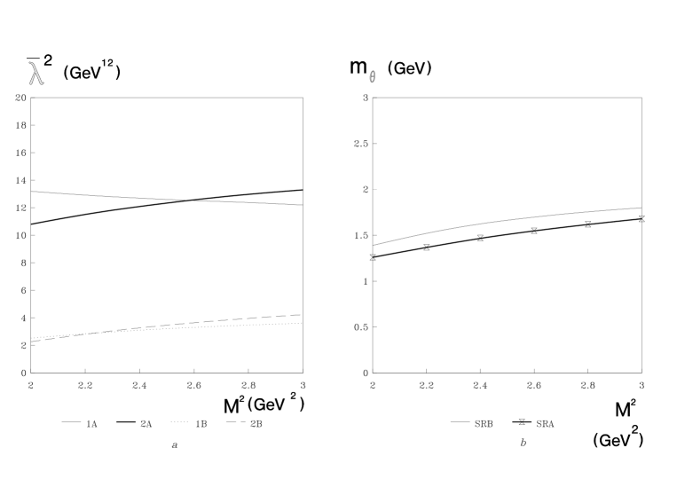
Figure 2: a)Sum rules (eqs.21,22) for currents $j^{A}$ (1A and 2A correspondingly) and $j^{b}$ (1B,2B). b) the pentaquark mass obtained as ratio eq.22/eq.21 (marked SRA)for currents $j^{A}$ and the same for currents $j^{B}$

The values of $\bar{\lambda}^{2}$, determined from eqs.(21) and (22) with the continuum threshold chosen as $s_{0}=3.5GeV^{2}$ are plotted in Fig.2a for the value of $m_{\theta}=1.54GeV$, and the value of $m_{\theta}$ obtained as a ratio of (22) to (21) is plotted in Fig.2b. The parameters were taken in accord with the recent determination of QCD condensates [21], [22] at normalization point $\mu^{2}=2GeV^{2}$: $a=0.63GeV^{3}$, $b=0.24GeV^{4}$, $m^{2}_{0}=0.8GeV^{2}$, $m_{s}=0.15GeV$, $\delta=0.8$.

We vary the value of the continuum threshold within the range 3-4.5$GeV^{2}$. One can easily see, that sum rules dependence on the Borel mass are rather stable (both SR1 and SR2) and also the value of the pentaquark mass is also stable enough. On the other side, the result strongly depends on the continuum threshold value. This fact is not unexpected, such strong dependence on the continuum threshold reflects the fact we have discussed before: in the pentaquark case the physical threshold of the first multiparticle state (nucleon plus kaon) in physical representation in physical representation of 2-point correlator, (which usually is much larger then first resonance and is included in the continuum), is even a little smaller than the mass of the first resonance (pentaquark $\theta^{+}$) mass. That’s why in the pentaquark case the ”continuum threshold” is just the free parameter, which can not be directly associated with higher resonance masses or physical multiparticle states threshold, and it will be fixed if one demands that the ratio of the 2-point sum rules $SR2/SR1$ should be equal to the experimental value. That’s why, it seems, that it is principally impossible to predict the pentaquark mass (unlike the case of usual hadrons)from 2-point sum rule for the pentaquark case. The only thing we can find from 2-point sum rule is: using the experimentally known value of mass, choose appropriate currents, which give reasonable sum rules (SR1 and SR2) and fix the such value of the parameter $s_{0}$ that the $SR2/SR1$ ratio becomes about pentaquark mass -if it is possible to do. (Of course, as soon as this parameter is fixed, it will be used in any other sum rule with this current, according to the usual logic of the sum rule approach). So we see, that for our case we can conclude that both currents $j_{a}$ $j_{b}$ can be treated as candidates to pentaquark current, because they give sum rule with a good stability and agree with experimental value of the pentaquark mass at $s_{0}$ about 3.5$GeV^{2}$, but one can’t say, that sum rules (21,22) themselves predict the pentaquark existence.

And yet, surprisingly, it was found to be possible to get more information from 2-point correlator and get some predictions about pentaquark. We will discuss this in the next section.

4. The estimation to the $KN$ contribution to the sum rules

The main question we try to answer in this section is: is it possible to explain the experimental results as some coupled baryon-meson system without any one-particle intermediate state. Let us suppose now, that the size of the $NK$ system (nucleon and kaon), is not too large (less than 0.5fm), so it can be extrapolated by some interpolating current (just the same as for pentaquark). To account the fact that this $NK$ system is not local let us define

$$\langle 0\mid\eta\mid nk\rangle=(\alpha\hat{P}+\beta m)\gamma_{5}v_{n}$$ (25)

where $\alpha$, $\beta$ are two unknown formfactors, $P$ is the four-moment, carried by nuclon-kaon system, and $v_{n}$ is nucleon spinor and $m$ is nucleon mass. It is clear, that if we will be interested in the region of the order of the pentaquark mass 1.54GeV, which is close to $(m_{n}+m_{k})^{2}$, (where $m_{n}$ and $m_{k}$ are nucleon and kaon masses correspondingly), one can suppose that formfactors are more or less constant in this region.

Then, substituting (25) into the relation $Im\Pi=\sum\langle 0\mid\eta\mid nk\rangle\langle nk\mid\bar{\eta}\mid 0\rangle+cont$

and integrating of the all intermediate states momenta, one can easily obtain for physical part of sum rules

$$Im\Pi=\hat{P}\rho_{1}(u)+m\rho_{2}(u)+\mbox{cont.contr}$$ (26)

where

$$u=P^{2},~{}\rho_{1}=\frac{c}{8\pi}\alpha^{2}\biggl{(}\frac{u}{2}-m^{2}\biggl{(}1-\frac{(1-z)^{2}}{2}\biggr{)}-\frac{m^{2}_{k}}{2}+\frac{z^{2}m^{2}(m^{2}-m^{2}_{k})}{2u}\biggr{)}$$ (27)

,

$$\rho_{2}=\frac{c}{8\pi}\alpha^{2}((z-1)m(u-zm^{2})-zm\cdot m^{2}_{k})$$ (28)

,

and $z=\beta/\alpha$, $c=\sqrt{(1-(m_{n}^{2}+m_{k}^{2})/u)^{2}-(2m_{n}m_{k}/u)^{2}}$

Then after Borel transformation one can easily write sum rules for both kinematical structures in the form, analogous to (21,22), where all notations of the left QCD side were defined in (23,24).

$$K_{1}^{(A,B)}\biggl{[}\overline{E}_{5}+R^{(A,B)}_{4}\overline{E}_{3}+R^{(A,B)}_{6}\overline{E}_{2}+R^{(A,B)}_{8}\overline{E}_{1}+R^{(A,B)}_{10}\overline{E}_{0}+$$

$$+R^{(A,B)}_{12}/M^{2}+R^{(A,B)}_{14}/M^{4}\biggr{]}\frac{M^{2}}{(4\pi)^{8}}=\int\limits^{s_{0}}_{(m_{n}+m_{k})^{2}}due^{-u/M^{2}}\rho_{1}/\pi$$ (29)

$$K_{2}^{(A,B)}\biggl{[}R^{(A,B)}_{1}\overline{E}_{5}+R^{(A,B)}_{3}\overline{E}_{4}+R^{(A,B)}_{5}\overline{E}_{3}+R^{(A,B)}_{7}\overline{E}_{2}+R_{9}^{(A,B)}\overline{E}_{1}+$$

$$+R^{(A,B)}_{11}\overline{E}_{0}+R^{(A,B)}_{13}/M^{2}\biggr{]}\frac{M^{2}}{(4\pi)^{8}}=\int\limits^{s_{0}}_{(m_{n}+m_{k})^{2}}due^{-u/M^{2}}\rho_{2}/\pi$$ (30)

On the other side at the pure $SU3_{f}$ chiral limit ( when the mass of kaon is zero) and the momentum of kaon $q=0$ the matrix element (25) should tend to zero. It can be easily shown using the equation of motion, that then for formfactors we have the relation $\alpha=\beta$. Because in our case we are interesting at physical region about pentaquark mass, which is close to $NK$ system generation threshold $(m_{n}+m_{k})^{2}$, then all momentum of particles are rather small and it is reasonable to demand that formfactors can differ at the same order as $SU3_{f}$ violation, i.e. about $30\%$.

So for each current we obtain two different sum rules, and the question is: is it possible to find such values of formfactors (more or less of the same value, i.e $z$ vary at 0.7 to 1.3, and $\alpha$ is free), which satisfy both sum rules (29,30). (One should note, that the parameter $s_{0}$ in this case is not the same as for the sum rules for the pentaquark case; we will vary it, but, of course, not very far from the pentaquark mass square region). The numerical analysis shows, that for both currents (19,20) it found to be impossible to satisfy sum rules (29) and (30) at the same time for all reliable values of $z$. For example in Fig.3a,b, the value $\xi$,

$$\xi=1/(4^{4}\pi^{3}\alpha)^{2}$$ (31)

,

obtained from SR1 (29) and SR2 (30)are shown for both choices of current $j^{A}$ (Fig.3a), and $j^{B}$ (Fig.3b), for the case $z=1.3$. One can see, that results of SR1 and SR2 totally contradict each other. For the smaller values of $z$ the contradiction becomes even more sronger (for example at $z=1$ the results of sum rules (29,30) strongly differ by modulo and moreover, have the opposite sign). So we can conclude, that the sum rules for the currents we consider indicate that to explain experimental results it is necessary to have some one-particle lower state (and pentaquark is a reliable candidate to this state) while the two-particle coupled lower state ($NK$ system) should be excluded .

4. Summary

The main results of this paper are the following:

1.The features of the sum rules for 2-point correlator with 5-quark currents are studied. It is shown, that on one side, the contributions of high dimension operators are significant, and, on the other side, the strong cancellation of the neighboring dimensions contribution should take place for any choice of the interpolating current. These features should be taken into account to obtain sum rules correctly, as is discussed in sect.2. The best way, from our point of view, is to take into account OPE series up to dimension 13,14, where one can neglect the cancellations.

2. Analysis of the sum rules for 2-point correlator with 5-quark currents for two different currents show, that it is impossible to explain the experimental result on pentaquark, supposing the existence only 2-particle lower state ($NK$ -system) in the physical representation of sum rules. For this reason one should suppose the existence of any one-particle lower state (like pentaquark) in this mass region. Obtained sum rules (21,22) have good stability and correspond to pentaquark mass $m_{\theta}$=1.54 $GeV$ at the appropriate choice of continuum threshold.

It is very necessary to note, that all conclusions and results are obtained without a possible instanton contribution. On the other side, it is well known, that the instanton contribution can be significant, especially at large dimension of OPE. (see [23] - [25])

That’s why the instanton contribution can influence the obtained results and conclusions and we are planning to investigate this problem in future.

Author thanks B.L. Ioffe for many significant advises and useful discussions.

This work is supported in part by US Civilian Research and Development Foundation (CRDF) Cooperative Grant Program, Project RUP2-2621-MO-04, RFBR grant 03-02-16209.

Figure 1: Examples of the diagrams, corresponding to the different operators contribution. Circles mean derivatives

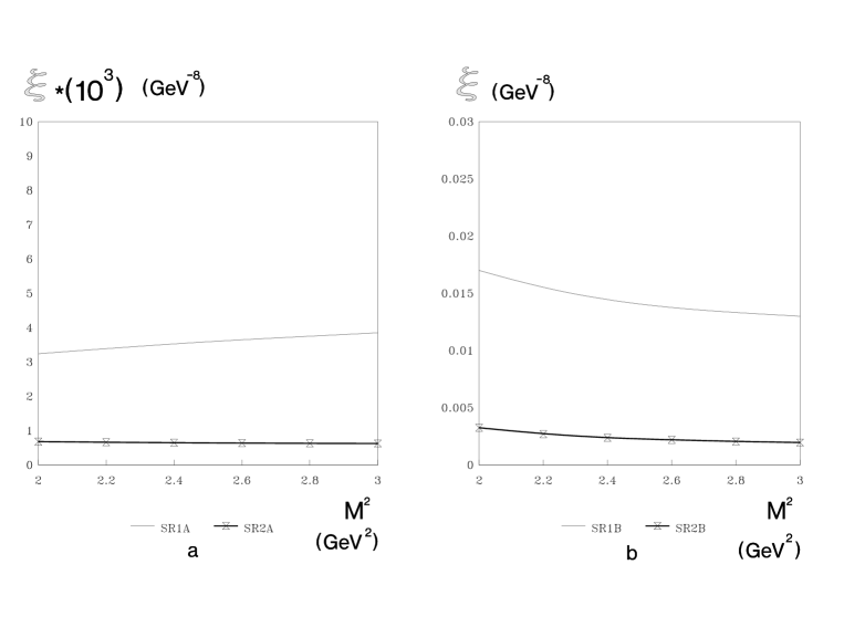
Figure 3: a) The value of $\xi$ (see eq.31) obtained from sum rules eq.29 (SR1A,) and eq.30 (SR2A) for current $j^{A}$ . b) the same for currents $j^{B}$

References

- [1] T.Nakano, D.S.Ahn, J.K.Ahn(LEPS Collaboration) et al., Phys.Rev.Lett. 91, 012002 (2003).
- [2] V.V.Barmin, V.S.Borisov A.G.Dolgolenko et al.(DIANA Collaboration), Yad.Fiz. 66, 1763 (2003). (Phys.At.Nucl. 66, 1715 (2003)).
- [3] 4. D.Diakonov, V.Petrov and M.Polaykov, Z.Phys. A359, 305 (1997).
- [4] K.Hicks,hep-ph/0408001.
- [5] R.A.Arndt, I.I.Strakovsky and R.L.Workman, nucl-th/0311030.
- [6] A.Sibirtsev, J.Heidenbauer , S.Krewald and Ulf-G.Meissner, hep-ph/0405099.
- [7] A.Sibirtsev, J.Heidenbauer, S.Krewald and Ulf-G.Meussner, nucl.th/0407011.
- [8] B.L.Ioffe and A.G.Oganesian, JETP Lett. B80 (2004), 386
- [9] A.G.Oganesian, hep-ph/0503193
- [10] R.D.Matheus and S.Narison,hep-ph/0412063
- [11] M.Eidemuller, F.S.Navarra, M.Nielsen and R.Rodrigues da Silva hep-ph/0503193
- [12] Zhi-Gang Wang, Wei-Min Yang, Shao-Long Wan and P.R.China hep-ph/0504151
- [13] B.L.Ioffe, Nucl.Phys. B188, 317(1981).
- [14] Shi-Lin Zhu, Phys.Rev.Lett. 91, 232002 (2003)
- [15] R.D.Matheus, F.S.Navarra, M.Nielsen et al. Phys.Lett. bf B578, 323 (2004).
- [16] J.J.Sugiyama, T.Doi and M.Oka, Phys.Lett. 581, 167 (2004).
- [17] M.Eidemuller, Phys.Lett B597 (2004), 314
- [18] Hee-Jang Lee. N.I.Kochelev, V.Vento hep-ph/0506250.
- [19] B.L.Ioffe and M.A.Shifman, Nucl.Phys. B202, 221 (1982).
- [20] B.L.Ioffe and A.V.Smilga, Nucl.Phys. B216, 373 (1983).
- [21] B.L.Ioffe and K.N.Zyablyuk, Nucl.Phys. A687, 437 (2001).
- [22] B.V.Geshkenbein, B.L.Ioffe and K.N.Zyablyuk, Phys.Rev. D64, 093009 (2001).
- [23] M.A.Shifman, A.I.Vainshtein and V.I.Zakharov Nucl.Phys. B147, 385,448 (1979).
- [24] V.A.Novikov,M.A.Shifman, A.I.Vainshtein and V.I.Zakharov Nucl.Phys. B249, 445 (1985).
- [25] B.V.Geshkenbein, B.L.Ioffe Nucl.Phys. B166, 340 (1980).