A posteriori inclusion of PDFs in NLO QCD final-state calculations

Abstract

Any NLO calculation of a QCD final-state observable involves Monte Carlo integration over a large number of events. For DIS and hadron colliders this must usually be repeated for each new PDF set, making it impractical to consider many ‘error’ PDF sets, or carry out PDF fits. Here we discuss “a posteriori” inclusion of PDFs, whereby the Monte Carlo run calculates a grid (in $x$ and $Q$) of cross section weights that can subsequently be combined with an arbitrary PDF. The procedure is numerically equivalent to using an interpolated form of the PDF. The main novelty relative to prior work is the use of higher-order interpolation, which substantially improves the tradeoff between accuracy and memory use. An accuracy of about $0.01$% has been reached for the single inclusive cross-section in the central rapidity region $|y|<0.5$ for jet transverse momenta from $100$ to $5000\mathrm{GeV}$. This method should facilitate the consistent inclusion of final-state data from HERA, Tevatron and LHC data in PDF fits, thus helping to increase the sensitivity of LHC to deviations from standard Model predictions.

1 Introduction

The Large Hadron Collider (LHC), currently under construction at CERN, will collide protons on protons with an energy of $7$ TeV. Together with its high collision rate the high available centre-of-mass energy will make it possible to test new interactions at very short distances that might be revealed in the production cross-sections of Standard Model (SM) particles at very high transverse momentum ($P_{T}$) as deviation from the SM theory.

The sensitivity to new physics crucially depends on experimental uncertainties in the measurements and on theoretical uncertainties in the SM predictions. It is therefore important to work out a strategy to minimize both the experimental and theoretical uncertainties from LHC data. For instance, one could use single inclusive jet or Drell-Yan cross-sections at low $P_{T}$ to constrain the PDF uncertainties at high $P_{T}$. Typical residual renormalisation and factorisation scale uncertainties in next-to-leading order (NLO) calculations for single inclusive jet-cross-section are about $5-10\%$ and should hopefully be reduced as NNLO calculations become available. The impact of PDF uncertainties on the other hand can be substantially larger in some regions, especially at large $P_{T}$, and for example at $P_{T}=2000$ GeV dominate the overall uncertainty of $20\%$. If a suitable combination of data measured at the Tevatron and LHC can be included in global NLO QCD analyses, the PDF uncertainties can be constrained.

The aim of this contribution is to propose a method for consistently including final-state observables in global QCD analyses.

For inclusive data like the proton structure function $F_{2}$ in deep-inelastic scattering (DIS) the perturbative coefficients are known analytically. During the fit the cross-section can therefore be quickly calculated from the strong coupling ($\alpha_{s}$) and the PDFs and can be compared to the measurements. However, final state observables, where detector acceptances or jet algorithms are involved in the definition of the perturbative coefficients (called “weights” in the following), have to be calculated using NLO Monte Carlo programs. Typically such programs need about one day of CPU time to calculate accurately the cross-section. It is therefore necessary to find a way to calculate the perturbative coefficients with high precision in a long run and to include $\alpha_{s}$ and the PDFs “a posteriori”.

To solve this problem many methods have been proposed in the past [1, 2, 3, 4, 4, 6]. In principle the highest efficiencies can be obtained by taking moments with respect to Bjorken-$x$ [1, 2], because this converts convolutions into multiplications. This can have notable advantages with respect to memory consumption, especially in cases with two incoming hadrons. On the other hand, there are complications such as the need for PDFs in moment space and the associated inverse Mellin transforms.

Methods in $x$-space have traditionally been somewhat less efficient, both in terms of speed (in the ‘a posteriori’ steps — not a major issue here) and in terms of memory consumption. They are, however, somewhat more transparent since they provide direct information on the $x$ values of relevance. Furthermore they can be used with any PDF. The use of $x$-space methods can be further improved by using methods developed originally for PDF evolution [7, 8].

2 PDF-independent representation of cross-sections

2.1 Representing the PDF on a grid

We make the assumption that PDFs can be accurately represented by storing their values on a two-dimensional grid of points and using $n^{\mathrm{th}}$-order interpolations between those points. Instead of using the parton momentum fraction $x$ and the factorisation scale $Q^{2}$, we use a variable transformation that provides good coverage of the full $x$ and $Q^{2}$ range with uniformly spaced grid points:

$$y(x)=\ln\frac{1}{x}\;\;\;{\rm and}\;\;\;\tau(Q^{2})=\ln\ln\frac{Q^{2}}{\Lambda^{2}}.$$ (1)

The parameter $\Lambda$ is to be chosen of the order of $\Lambda_{\mathrm{QCD}}$, but not necessarily identical. The PDF $q(x,Q^{2})$ is then represented by its values $q_{i_{y},i_{\tau}}$ at the 2-dimensional grid point $(i_{y}\,\delta y,i_{\tau}\,\delta\tau)$, where $\delta y$ and $\delta\tau$ denote the grid spacings, and obtained elsewhere by interpolation:

$$q(x,Q^{2})=\sum_{i=0}^{n}\sum_{\iota=0}^{n^{\prime}}q_{k+i,\kappa+\iota}\,\,I_{i}^{(n)}\left(\frac{y(x)}{\delta y}-k\right)\,I_{\iota}^{(n^{\prime})}\left(\frac{\tau(Q^{2})}{\delta\tau}-\kappa\right),$$ (2)

where $n$, $n^{\prime}$ are the interpolation orders. The interpolation function $I_{i}^{(n)}(u)$ is 1 for $u=i$ and otherwise is given by:

$$I_{i}^{(n)}(u)=\frac{(-1)^{n-i}}{i!(n-i)!}\frac{u(u-1)\ldots(u-n)}{u-i}\,.$$ (3)

Defining $\mathrm{int}(u)$ to be the largest integer such that $\mathrm{int}(u)\leq u$, $k$ and $\kappa$ are defined as:

$$k(x)= \mathrm{int}\left(\frac{y(x)}{\delta y}-\frac{n-1}{2}\right), \kappa(x)=\mathrm{int}\left(\frac{\tau(Q^{2})}{\delta\tau}-\frac{n^{\prime}-1}{2}\right).$$ (4)

Given finite grids whose vertex indices range from $0\ldots N_{y}-1$ for the $y$ grid and $0\ldots N_{\tau}-1$ for the $\tau$ grid, one should additionally require that eq. (2) only uses available grid points. This can be achieved by remapping $k\to\max(0,\min(N_{y}-1-n,k))$ and $\kappa\to\max(0,\min(N_{\tau}-1-n^{\prime},\kappa))$.

2.2 Representing the final state cross-section weights on a grid (DIS case)

Suppose that we have an NLO Monte Carlo program that produces events $m=1\dots N$. Each event $m$ has an $x$ value, $x_{m}$, a $Q^{2}$ value, $Q^{2}_{m}$, as well as a weight, $w_{m}$, and a corresponding order in $\alpha_{s}$, $p_{m}$. Normally one would obtain the final result $W$ of the Monte Carlo integration from:

$$W=\sum_{m=1}^{N}\,w_{m}\,\left(\frac{\alpha_{s}(Q_{m}^{2})}{2\pi}\right)^{p_{m}}\,q(x_{m},Q^{2}_{m}).$$ (5)

Instead one introduces a weight grid $W_{i_{y},i_{\tau}}^{(p)}$ and then for each event updates a portion of the grid with:
$i=0\dots n,\;\iota=0\dots n^{\prime}:$

$$W_{k+i,\kappa+\iota}^{(p_{m})}\to W_{k+i,\kappa+\iota}^{(p_{m})}+w_{m}\,I_{i}^{(n)}\left(\frac{y(x_{m})}{\delta y}-k\right)I_{\iota}^{(n^{\prime})}\left(\frac{\tau(Q^{2}_{m})}{\delta\tau}-\kappa\right),$$ (6)

$$\;\;\;{\rm where}\;\;\;k\equiv k(x_{m}),\;\kappa\equiv\kappa(Q^{2}_{m}).$$

The final result for $W$, for an arbitrary PDF, can then be obtained subsequent to the Monte Carlo run:

$$W=\sum_{p}\sum_{i_{y}}\sum_{i_{\tau}}W_{i_{y},i_{\tau}}^{(p)}\,\left(\frac{\alpha_{s}\left({Q^{2}}^{(i_{\tau})}\right)}{2\pi}\right)^{p}q\!\left(x^{(i_{y})},{Q^{2}}^{(i_{\tau})}\right)\,,$$ (7)

where the sums index with $i_{y}$ and $i_{\tau}$ run over the number of grid points and we have have explicitly introduced $x^{(i_{y})}$ and ${Q^{2}}^{(i_{\tau})}$ such that:

$$y(x^{(i_{y})})=i_{y}\,\delta y\quad{\rm and}\quad\tau\left({Q^{2}}^{(i_{\tau})}\right)=i_{\tau}\,\delta\tau.$$ (8)

2.3 Including renormalisation and factorisation scale dependence

If one has the weight matrix $W_{i_{y},i_{\tau}}^{(p)}$ determined separately order by order in $\alpha_{s}$, it is straightforward to vary the renormalisation $\mu_{R}$ and factorisation $\mu_{F}$ scales a posteriori (we assume that they were kept equal in the original calculation).

It is helpful to introduce some notation relating to the DGLAP evolution equation:

$$\frac{dq(x,Q^{2})}{d\ln Q^{2}}=\frac{\alpha_{s}(Q^{2})}{2\pi}(P_{0}\otimes q)(x,Q^{2})+\left(\frac{\alpha_{s}(Q^{2})}{2\pi}\right)^{2}(P_{1}\otimes q)(x,Q^{2})+\ldots,$$ (9)

where the $P_{0}$ and $P_{1}$ are the LO and NLO matrices of DGLAP splitting functions that operate on vectors (in flavour space) $q$ of PDFs. Let us now restrict our attention to the NLO case where we have just two values of $p$, $p_{\mathrm{LO}}$ and $p_{\mathrm{NLO}}$. Introducing $\xi_{R}$ and $\xi_{F}$ corresponding to the factors by which one varies $\mu_{R}$ and $\mu_{F}$ respectively, for arbitrary $\xi_{R}$ and $\xi_{F}$ we may then write:

$$W(\xi_{R},\xi_{F})=\sum_{i_{y}}\sum_{i_{\tau}}\left(\frac{\alpha_{s}\left(\xi_{R}^{2}{Q^{2}}^{(i_{\tau})}\right)\,}{2\pi}\right)^{p_{\mathrm{LO}}}W_{i_{y},i_{\tau}}^{(p_{\mathrm{LO}})}q\!\left(x^{(i_{y})},\xi_{F}^{2}{Q^{2}}^{(i_{\tau})}\right)+$$

$$\left(\frac{\alpha_{s}\left(\xi_{R}^{2}{Q^{2}}^{(i_{\tau})}\right)\,}{2\pi}\right)^{p_{\mathrm{NLO}}}\left[\left(W_{i_{y},i_{\tau}}^{(p_{\mathrm{NLO}})}+2\pi\beta_{0}p_{\mathrm{LO}}\ln\xi_{R}^{2}\,W_{i_{y},i_{\tau}}^{(p_{\mathrm{LO}})}\right)q\!\left(x^{(i_{y})},\xi_{F}^{2}{Q^{2}}^{(i_{\tau})}\right)\right.$$ (10)

$$\left.-\ln\xi_{F}^{2}\,W_{i_{y},i_{\tau}}^{(p_{\mathrm{LO}})}(P_{0}\otimes q)\!\left(x^{(i_{y})},\xi_{F}^{2}{Q^{2}}^{(i_{\tau})}\right)\right]\,,$$

where $\beta_{0}=(11N_{c}-2n_{f})/(12\pi)$ and $N_{c}$ ($n_{f}$) is the number of colours (flavours). Though this formula is given for $x$-space based approach, a similar formula applies for moment-space approaches. Furthermore it is straightforward to extend it to higher perturbative orders.

2.4 Representing the weights in the case of two incoming hadrons

In hadron-hadron scattering one can use analogous procedures with one more dimension. Besides $Q^{2}$, the weight grid depends on the momentum fraction of the first ($x_{1}$) and second ($x_{2}$) hadron.

In the case of jet production in proton-proton collisions the weights generated by the Monte Carlo program as well as the PDFs can be organised in seven possible initial state combinations of partons:

$$\mathrm{gg}:\;\;F^{(0)}(x_{1},x_{2};Q^{2}) = G_{1}(x_{1})G_{2}(x_{2})$$ (11)

$$\mathrm{qg}:\;\;F^{(1)}(x_{1},x_{2};Q^{2}) = \left(Q_{1}(x_{1})+\overline{Q}_{1}(x_{1})\right)G_{2}(x_{2})$$ (12)

$$\mathrm{gq}:\;\;F^{(2)}(x_{1},x_{2};Q^{2}) = G_{1}(x_{1})\left(Q_{2}(x_{2})+\overline{Q}_{2}(x_{2})\right)$$ (13)

$$\mathrm{qr}:\;\;F^{(3)}(x_{1},x_{2};Q^{2}) = Q_{1}(x_{1})Q_{2}(x_{2})+\overline{Q}_{1}(x_{1})\overline{Q}_{2}(x_{2})-D(x_{1},x_{2})$$ (14)

$$\mathrm{qq}:\;\;F^{(4)}(x_{1},x_{2};Q^{2}) = D(x_{1},x_{2})$$ (15)

$$\mathrm{q\bar{q}}:\;\;F^{(5)}(x_{1},x_{2};Q^{2}) = \overline{D}(x_{1},x_{2})$$ (16)

$$\mathrm{q\bar{r}}:\;\;F^{(6)}(x_{1},x_{2};Q^{2}) = Q_{1}(x_{1})\overline{Q}_{2}(x_{2})+\overline{Q}_{1}(x_{1})Q_{2}(x_{2})-\overline{D}(x_{1},x_{2}),$$ (17)

where $g$ denotes gluons, $q$ quarks and $r$ quarks of different flavour $q\neq r$ and we have used the generalized PDFs defined as:

$$G_{H}(x)=f_{0/H}(x,Q^{2}), Q_{H}(x)=\sum_{i=1}^{6}f_{i/H}(x,Q^{2}),\;\;\overline{Q}_{H}(x)=\sum_{i=-6}^{-1}f_{i/H}(x,Q^{2}),$$

$$D(x_{1},x_{2}) = \mathop{\sum_{i=-6}^{6}}_{i\neq 0}f_{i/H_{1}}(x_{1},Q^{2})f_{i/H_{2}}(x_{2},Q^{2}),$$ (18)

$$\overline{D}(x_{1},x_{2},\mu^{2}_{F}) = \mathop{\sum_{i=-6}^{6}}_{i\neq 0}f_{i/H_{1}}(x_{1},Q^{2})f_{-i/H_{2}}(x_{2},Q^{2}),\;\;$$

where $f_{i/H}$ is the PDF of flavour $i=-6\dots 6$ for hadron $H$ and $H_{1}$ ($H_{2}$) denotes the first or second hadron.

The analogue of eq. 7 is then given by:

$$W=\sum_{p}\sum_{l=0}^{6}\sum_{i_{y_{1}}}\sum_{i_{y_{2}}}\sum_{i_{\tau}}W_{i_{y_{1}},i_{y_{2}},i_{\tau}}^{(p)(l)}\,\left(\frac{\alpha_{s}\left({Q^{2}}^{(i_{\tau})}\right)}{2\pi}\right)^{p}F^{(l)}\left(x_{1}^{(i_{y_{1}})},x_{2}^{(i_{y_{1}})},{Q^{2}}^{(i_{\tau})}\right).$$ (19)

2.5 Including scale depedence in the case of two incoming hadrons

It is again possible to choose arbitrary renormalisation and factorisation scales, specifically for NLO accuracy:

$$W(\xi_{R},\xi_{F})=\sum_{l=0}^{6}\sum_{i_{y_{1}}}\sum_{i_{y_{2}}}\sum_{i_{\tau}}\left(\frac{\alpha_{s}\left(\xi_{R}^{2}{Q^{2}}^{(i_{\tau})}\right)\,}{2\pi}\right)^{p_{\mathrm{LO}}}W_{i_{y_{1}},i_{y_{2}},i_{\tau}}^{(p_{\mathrm{LO}})(l)}F^{(l)}\left(x_{1}^{(i_{y_{1}})},x_{2}^{(i_{y_{1}})},\xi_{F}^{2}{Q^{2}}^{(i_{\tau})}\right)+$$

$$\left(\frac{\alpha_{s}\left(\xi_{R}^{2}{Q^{2}}^{(i_{\tau})}\right)\,}{2\pi}\right)^{p_{\mathrm{NLO}}}\left[\left(W_{i_{y_{1}},i_{y_{2}},i_{\tau}}^{(p_{\mathrm{NLO}})(l)}+2\pi\beta_{0}p_{\mathrm{LO}}\ln\xi_{R}^{2}\,W_{i_{y_{1}},i_{y_{2}},i_{\tau}}^{(p_{\mathrm{LO}})(l)}\right)F^{(l)}\left(x_{1}^{(i_{y_{1}})},x_{2}^{(i_{y_{1}})},\xi_{F}^{2}{Q^{2}}^{(i_{\tau})}\right)\right.$$ (20)

$$\left.-\ln\xi_{F}^{2}\,W_{i_{y_{1}},i_{y_{2}},i_{\tau}}^{(p_{\mathrm{LO}})(l)}\left(F^{(l)}_{q_{1}\to P_{0}\otimes q_{1}}\left(x_{1}^{(i_{y_{1}})},x_{2}^{(i_{y_{1}})},\xi_{F}^{2}{Q^{2}}^{(i_{\tau})}\right)+F^{(l)}_{q_{2}\to P_{0}\otimes q_{2}}\left(x_{1}^{(i_{y_{1}})},x_{2}^{(i_{y_{1}})},\xi_{F}^{2}{Q^{2}}^{(i_{\tau})}\right)\right)\right]\,,$$

where $F^{(l)}_{q_{1}\to P_{0}\otimes q_{1}}$ is calculated as $F^{(l)}$, but with $q_{1}$ replaced wtih $P_{0}\otimes q_{1}$, and analogously for $F^{(l)}_{q_{2}\to P_{0}\otimes q_{2}}$.

3 Technical implementation

To test the scheme discussed above we use the NLO Monte Carlo program NLOJET++ [10] and the CTEQ6 PDFs [13]. The grid $W_{i_{y_{1}},i_{y_{2}},i_{\tau}}^{(p)(l)}$ of eq. 19 is filled in a NLOJET++ user module. This module has access to the event weight and parton momenta and it is here that one specifies and calculates the physical observables that are being studied (e.g. jet algorithm).

Having filled the grid we construct the cross-section in a small standalone program which reads the weights from the grid and multiplies them with an arbitrary $\alpha_{s}$ and PDF according to eq. 19. This program runs very fast (in the order of seconds) and can be called in a PDF fit.

The connection between these two programs is accomplished via a C++ class, which provides methods e.g. for creating and optimising the grid, filling weight events and saving it to disk. The classes are general enough to be extendable for the use with other NLO calculations.

The complete code for the NLOJET++ module, the C++ class and the standalone job is available from the authors. It is still in a development, testing and tuning stage, but help and more ideas are welcome.

3.1 The C++ class

The main data members of this class are the grids implemented as arrays of three-dimensional ROOT histograms, with each grid point at the bin centers:

$${\rm TH3D[p][l][iobs](x_{1},x_{2},Q^{2})},$$ (21)

where the $l$ and $p$ are explained in eq. 19 and $iobs$ denotes the observable bin, e.g. a given $P_{T}$ range.

The C++ class initialises, stores and fills the grid using the following main methods:

• Default constructor: Given the pre-defined kinematic regions of interest, it initializes the grid.

• Optimizing method: Since in some bins the weights will be zero over a large kinematic region in $x_{1},x_{2},Q^{2}$, the optimising method implements an automated procedure to adapt the grid boundaries for each observable bin. These boundaries are calculated in a first (short) run. In the present implementation, the optimised grid has a fixed number of grid points. Other choices, like a fixed grid spacing, might be implemented in the future.

• Loading method: Reads the saved weight grid from a ROOT file

• Saving method: Saves the complete grid to a ROOT file, which will be automatically compressed.

3.2 The user module for NLOJET++

The user module has to be adapted specifically to the exact definition of the cross-section calculation. If a grid file already exists in the directory where NLOJET++ is started, the grid is not started with the default constructor, but with the optimizing method (see 3.1). In this way the grid boundaries are optimised for each observable bin. This is necessary to get very fine grid spacings without exceeding the computer memory. The grid is filled at the same place where the standard NLOJET++ histograms are filled. After a certain number of events, the grid is saved in a root-file and the calculation is continued.

3.3 The standalone program for constructing the cross-section

The standalone program calculates the cross-section in the following way:

1. Load the weight grid from the ROOT file

2. Initialize the PDF interface, load $q(x,Q^{2})$ on a helper PDF-grid (to increase the performance)

3. For each observable bin, loop over $i_{y_{1}},i_{y_{2}},i_{\tau},l,p$ and calculate $F^{l}(x_{1},x_{2},Q^{2})$ from the appropriate PDFs $q(x,Q^{2})$, multiply $\alpha_{s}$ and the weights from the grid and sum over the initial state parton configuration $l$, according to eq. 19.

4 Results

We calculate the single inclusive jet cross-section as a function of the jet transverse momentum ($P_{T}$) for jets within a rapidity of $|y|<0.5$. To define the jets we use the seedless cone jet algorithm as implemented in NLOJET++ using the four-vector recombination scheme and the midpoint algorithm. The cone radius has been put to $R=0.7$, the overlap fraction was set to $f=0.5$. We set the renormalisation and factorization scale to $Q^{2}=P_{T,max}^{2}$, where $P_{T,max}$ is the $P_{T}$ of the highest $P_{T}$ jet in the required rapidity region.

In our test runs, to be independent from statistical fluctuations (which can be large in particular in the NLO case), we fill in addition to the grid a reference histogram in the standard way according to eq. 5.

The choice of the grid architecture depends on the required accuracy, on the exact cross-section definition and on the available computer resources. Here, we will just sketch the influence of the grid architecture and the interpolation method on the final result. We will investigate an example where we calculate the inclusive jet cross-section in $N_{\mathrm{obs}}=100$ bins in the kinematic range $100\,\leq P_{T}\leq 5000\,\mathrm{GeV}$. In future applications this can serve as guideline for a user to adapt the grid method to his/her specific problem. We believe that the code is transparent and flexible enough to adapt to many applications.

As reference for comparisons of different grid architectures and interpolation methods we use the following:

• Grid spacing in $y(x)$: $10^{-5}\leq x_{1},x_{2}\leq 1.0$ with $N_{y}=30$

• Grid spacing in $\tau(Q^{2})$: $100\,\mathrm{GeV}\leq Q\leq 5000\,\mathrm{GeV}$ with $N_{\tau}=30$

• Order of interpolation: $n_{y}=3,\,n_{\tau}=3$

The grid boundaries correspond to the user setting for the first run which determines the grid boundaries for each observable bin. In the following we call this grid architecture $30^{2}$x$30$x$100(3,3)$. Such a grid takes about $300$ Mbyte of computer memory. The root-file where the grid is stored has about $50$ Mbyte.

The result is shown in Fig. 1a). The reference cross-section is reproduced everywhere to within $0.05\%$. The typical precision is about $0.01\%$. At low and high $P_{T}$ there is a positive bias of about $0.04\%$. Also shown in Fig. 1a) are the results obtained with different grid architectures. For a finer $x$ grid ($50^{2}$x$30$x$100(3,3)$) the accuracy is further improved (within $0.005\%$) and there is no bias. A finer ($30^{2}$x$60$x$100(3,3)$) as well as a coarser ($30^{2}$x$10$x$100(3,3)$) binning in $Q^{2}$ does not improve the precision.

Fig. 1b) and Fig. 1c) show for the grid ($30^{2}$x$30$x$100$) different interpolation methods. With an interpolation of order $n=5$ the precision is $0.01\%$ and the bias at low and high $P_{T}$ observed for the $n=3$ interpolation disappears. The result is similar to the one obtained with finer $x$-points. Thus by increasing the interpolation order the grid can be kept smaller. An order $n=1$ interpolation gives a systematic negative bias of about $1\%$ becoming even larger towards high $P_{T}$.

Depending on the available computer resources and the specific problem, the user will have to choose a proper grid architecture. In this context, it is interesting that a very small grid $10^{2}$x$10$x$100(5,5)$ that takes only about $10$ Mbyte computer memory reaches still a precision of $0.5\%$, if an interpolation of order $n=5$ is used (see Fig. 1d)).

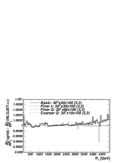
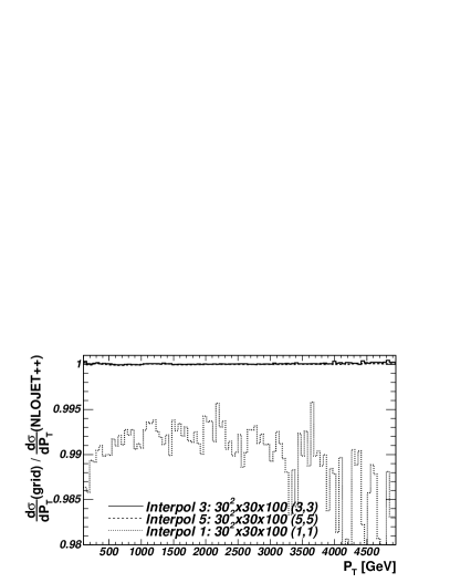
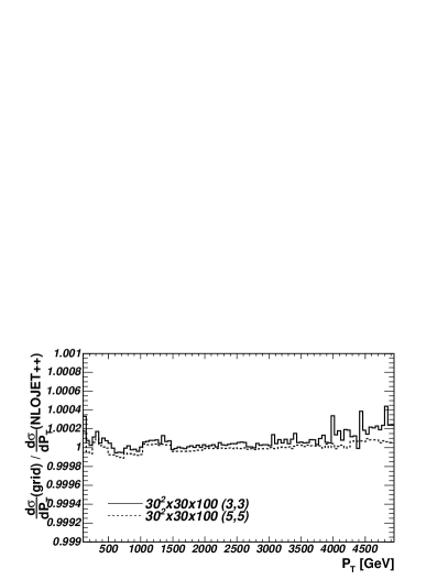
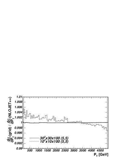
Figure 1: Ratio between the single inclusive jet cross-section with $100$ $P_{T}$ bins calculated with the grid technique and the reference cross-section calculated in the standard way. Shown are the standard grid, grids with finer $x$ and $Q^{2}$ sampling (a) with interpolation of order $1$, $3$ and $5$ (b) (and on a finer scale in c)) and a small grid (d).

5 Conclusions

We have developed a technique to store the perturbative coefficients calculated by an NLO Monte Carlo program on a grid allowing for a-posteriori inclusion of an arbitrary parton density function (PDF) set. We extended a technique that was already successfully used to analyse HERA data to the more demanding case of proton-proton collisions at LHC energies.

The technique can be used to constrain PDF uncertainties, e.g. at high momentum transfers, from data that will be measured at LHC and allows the consistent inclusion of final state observables in global QCD analyses. This will help increase the sensitivity of LHC to find new physics as deviations from the Standard Model predictions.

Even for the large kinematic range for the parton momentum fractions $x_{1}$ and $x_{2}$ and of the squared momentum transfer $Q^{2}$ accessible at LHC, grids of moderate size seem to be sufficient. The single inclusive jet cross-section in the central region $|y|<0.5$ can be calculated with a precision of $0.01\%$ in a realistic example with $100$ bins in the transverse jet energy range $100\,\leq P_{T}\leq 5000\,\mathrm{GeV}$. In this example, the grid occupies about $300$ Mbyte computer memory. With smaller grids of order $10$ Mbyte the reachable accuracy is still $0.5\%$. This is probably sufficient for all practical applications.

References

- [1] D. Graudenz, M. Hampel, A. Vogt and C. Berger, Z. Phys. C 70, 77 (1996)
- [2] D. A. Kosower, Nucl. Phys. B 520, 263 (1998)
- [3] M. Stratmann and W. Vogelsang, Phys. Rev. D64, 114007 (2001)
- [4] M. Wobisch, PhD-thesis RWTH Aachen, PITHA 00/12 and DESY-THESIS-2000-049
- [5] C. Adloff et al. (H1 Collab.), Eur. Phys. J. C19, 289 (2001)
- [6] S. Chekanov et al. (ZEUS Collab.) (2005)
- [7] P. G. Ratcliffe, Phys. Rev. D 63, 116004 (2001)
- [8] M. Dasgupta and G. P. Salam, Eur. Phys. J. C 24, 213 (2002)
- [9] S. Eidelman. et al., Phys. Lett. B592, 1 (2004)
- [10] Z. Nagy, Phys. Rev. D68, 094002 (2003)
- [11] Z. Nagy, Phys. Rev. Lett. 88, 122003 (2002)
- [12] Z. Nagy and Z. Trocsanyi, Phys. Rev. Lett. 87, 082001 (2001)
- [13] J. Pumplin et al. (CTEQ collab.), JHEP 07, 012 (2002)
- [14] M. R. Whalley, D. Bourilkov and R. C. Group, these proceedings (2005).