Signals of a Weibel Instability in the Melting Color Glass Condensate

Abstract

Based on hep-ph/0510121, we discuss further the numerical study of classical SU(2) 3+1-D Yang-Mills equations for matter produced in a high energy heavy ion collision. The growth of the amplitude of fluctuations as $\exp{(\Gamma\sqrt{g^{2}\mu\tau})}$ (where $g^{2}\mu$ is a scale arising from the saturation of gluons in the nuclear wavefunction) is shown to be robust over a wide range of initial amplitudes that violate boost invariance. We argue that this growth is due to a non-Abelian Weibel instability, the scale of which is set by a dynamically generated plasmon mass. We discuss the relation of $\Gamma$ to the prediction from kinetic theory.

1 Introduction

One objective of the experiments done at ultra-relativistic heavy-ion colliders such as RHIC and, in future, the LHC, is to understand the properties of very hot and dense partonic matter in QCD. This requires understanding how the coherent wavefunctions of the incoming nuclei decohere, possibly forming a thermal Quark Gluon Plasma (QGP). At high energies, the small x (or wee) partons determine the properties of nuclear wavefunctions. Their properties can be formulated in an effective field theory called the Color Glass Condensate (CGC) [1]. A semi-hard scale $Q_{s}(x)>>\Lambda_{\rm QCD}$, the “saturation” scale [2], arises naturally in this approach and grows with energy; weak coupling techniques are therefore feasible. Furthermore , the small x wavefunctions of the incoming nuclei can be treated as classical fields with large occupation numbers [3]. This enables the description of nuclear collisions in terms of solutions of classical Yang-Mills equations with the fields representing the small x partons, and light cone currents describing the hard valence partons [4]. The latter can be modeled as

$$J^{\mu}=\delta^{\mu+}\rho_{1}(x_{\perp})\delta(x^{-})+\delta^{\mu-}\rho_{2}(x_{\perp})\delta(x^{+}),$$ (1)

where the color charge densities $\rho_{1,2}$ of the two nuclei are independent sources of color charge ($x^{\pm}=(t\pm z)/2$). The $\delta$-function sources ensure that the fields are boost invariant, namely, independent of the space time rapidity $\eta$, defined as $\eta={\rm atanh{(z/t)}}$. The Yang-Mills equations can therefore be expressed in terms of the two transverse directions (${\bf x}_{\perp}$) and the proper time $\tau$, defined as $\tau=\sqrt{t^{2}-z^{2}}$. The initial conditions can be determined by matching the Yang-Mills equation in the four light cone regions, at $\tau=0$, to determine self-consistently the fields in the forward light cone in terms of those before the collision. These latter classical fields can be computed analytically in the CGC framework.

In the McLerran-Venugopalan model (MV) [3] for large nuclei, the sources of color charge are Gaussian distributed

$$\langle\rho_{i}^{a}({\bf x}_{\perp})\rho_{j}^{b}({\bf y}_{\perp})\rangle=g^{4}\mu^{2}\delta_{ij}\delta^{ab}\delta^{2}({\bf x_{\perp}}-{\bf y_{\perp}})\,,$$ (2)

where $g^{2}\mu$ is the dimensionful momentum scale in the problem. This scale is closely related to the saturation scale $Q_{s}$ which, in the classical effective theory, is defined as $Q_{s}^{2}=g^{4}\mu^{2}N_{c}\ln(g^{2}\mu/\Lambda_{\rm QCD})/2\pi$. For the initial conditions corresponding to configurations of color sources of each of the two nuclei, the Yang-Mills equations can be solved numerically, and the final gauge field configurations averaged over the sources, to determine energy and number distributions [5].

It is clear that for all finite $\sqrt{s}$ the ansatz of $\delta$-function sources in Eq. (1) has to be modified in order to implement the fact that the nuclei will not be contracted into infinitely thin sheets. More important, however, are the effects of quantum corrections, which may be of order unity over rapidity scales $\sim 1/\alpha_{s}$. These are not included in the MV model but arise from small x quantum evolution of the classical fields [1]. Consequently, one must deal with functions having a finite width in $x^{\pm}$, respectively. For a single nucleus it is still possible to solve the Yang-Mills equations classically and obtain the Weizsäcker-Williams fields. For two nuclei, however, the problem becomes more involved, simply because the nuclei will interact for a finite time and the single nucleus solutions before the collision will be distorted during this time span. Ignoring the details of this process, the main difference with respect to the cases considered so far [5] will be the emergence of rapidity fluctuations and consequently a breaking of the boost-invariance of the small x fields. In what follows, we will concentrate on studying the effect of rapidity fluctuations by numerically solving the Yang-Mills equations after the collision (based on Ref.[6]); to keep the analysis as simple as possible, we assume the initial distortions of exact boost-invariance to be very small. The reasons for this are two-fold. One is to connect our results to published results [5]. The other reason, as we will discuss, is to study the effects of the Weibel instabilities over several decades in the magnitudes of amplitudes.

This work is organized as follows: In section 2 we discuss why this study is connected to the phenomenon of non-Abelian plasma instabilities ([7, 8, 9, 10, 11, 12]), before providing details of our setup in section 3. Our results are presented in section 4.

2 Motivation

At earliest times $\tau Q_{s}\leq 1$, typical gluon occupation numbers are large and thus the system is described most appropriately in terms of nonlinear gluonic fields, which should be accessible by simulating classical Yang-Mills dynamics [5]. However, because of the rapid longitudinal expansion, the gluon occupation number drops until the non-linearities become so weak that the hard modes ($p\sim Q_{s}$) can be described as on-shell particles. In this regime (which should be reached for $\tau Q_{s}\geq 1$), the dynamics of the system is in terms of hard particles coupled to soft ($k\ll gQ_{s}$) fields, so a Vlasov-type kinetic approach should be appropriate to describe the system. Consequently, at times $\tau Q_{s}\sim 1$, one would expect both classical and kinetic theory descriptions to offer a fair approximation of the system dynamics.

Another consequence of the longitudinal expansion is that the typical longitudinal gluon momentum, for a fixed slice in rapidity, becomes smaller as $p_{z}\sim 1/\tau$. Since the transverse gluon momentum stays approximately constant $p_{\perp}\sim Q_{s}$, the gluon distribution function $f({\bf p})$ tends to become more and more anisotropic (until scatterings become important at very late times).

Using a Vlasov approach it has been shown [7, 8, 9, 10, 11, 12] that when expansion effects are negligible, systems with an anisotropic momentum-space distribution function are subject to the presence of so-called plasma-instabilities, with a typical exponential growth rate $\gamma$ proportional to the soft scale $m_{\infty}$,

$$\gamma\sim\frac{m_{\infty}}{\sqrt{2}},\qquad m_{\infty}^{2}=g^{2}N_{c}\int\frac{d^{3}p}{(2\pi)^{3}}\frac{f({\bf p})}{|{\bf p}|}$$ (3)

in the limit of very strong anisotropies [9]. These instabilities manifest themselves as exponentially growing magnetic fields which in turn reduce the momentum-anisotropy, both by transferring energy from hard to soft excitations as well as by bending hard particle trajectories.

Because of the relation between classical field dynamics and kinetic theory at times $\tau Q_{s}\sim 1$ conjectured above, one would expect to see some manifestation of these instabilities when simulating classical Yang-Mills dynamics. To simulate an expanding metric, we solve the Yang-Mills equations in $(\tau,\eta,{\bf x}_{\perp})$ co-ordinates. In momentum space, the conjugate momenta are $(k^{\tau},k_{\eta},{\bf k}_{\perp})$, respectively. The Yang-Mills fields for “soft” $k_{\eta}$ modes will thus be sensitive to anisotropic distributions of modes in (${\bf k}_{\perp}$,$k_{\eta}$), thereby triggering an instability of the Weibel type. It was predicted by Arnold, Lenaghan and Moore [9] that in an expanding system such an instability would grow as $\exp\left(\sqrt{\tau}\right)$ rather than $\exp(\tau)$. As shown in Ref. [6], this is precisely what happens. Below, we discuss in some detail the setup of the numerical problem and some of the results.

3 Setup

In $A^{\tau}=0$ gauge, the gluonic part of the QCD action has the form [5]

$$S=\int d\tau d\eta dx_{\perp}\tau{\rm Tr}\left[\frac{F_{\tau\eta}^{2}}{\tau^{2}}+F_{\tau i}^{2}-\frac{F_{\eta i}^{2}}{\tau^{2}}-\frac{F_{ij}^{2}}{2}+\frac{j_{\eta}A_{\eta}}{\tau^{2}}\right]=\int d\tau d\eta dx_{\perp}{\mathcal{L}},$$ (4)

where $F_{\mu\nu}=\partial_{\mu}A_{\nu}-\partial_{\nu}A_{\mu}+ig[A_{\mu},A_{\nu}]$ is the field strength in the fundamental representation with $F^{\mu\nu}=F^{\mu\nu}_{a}\tau_{a}$ and $[\tau_{a},\tau_{b}]=if_{abc}\tau_{c}$, ${\rm Tr}\ \tau^{a}\tau^{b}=\frac{\delta_{ab}}{2}$. In the following we shall ignore effects of the current $j_{\eta}$. This is justified if we limit ourselves to a small region around $\eta=0$. With this restriction in mind we derive the conjugate momenta from the Lagrangian Eq.(4),

$$E_{i}=\frac{\partial{\mathcal{L}}}{\partial(\partial_{\tau}A_{i})}=\tau\partial_{\tau}A_{i},\qquad E_{\eta}=\frac{\partial{\mathcal{L}}}{\partial(\partial_{\tau}A_{\eta})}=\frac{1}{\tau}\partial_{\tau}A_{\eta}$$ (5)

with which we construct the Hamiltonian density

$${\mathcal{H}}=E_{i}(\partial_{\tau}A_{i})+E_{\eta}(\partial_{\tau}A_{\eta})-{\mathcal{L}}={\rm Tr}\ \left[\frac{E_{i}^{2}}{\tau}+\frac{F_{\eta i}^{2}}{\tau}+\tau E_{\eta}^{2}+\tau F_{xy}^{2}\right].$$ (6)

Here transverse coordinates $x,y$ have been collectively labeled by the Latin index $i$. Using finally $\partial{\mathcal{H}}/\partial E_{\mu}=\partial_{\tau}A_{\mu},\ \partial{\mathcal{H}}/\partial A_{\mu}=-\partial_{\tau}E_{\mu}\,,$ Hamilton’s equations for the fields and their conjugate momenta are

$$\partial_{\tau}A_{i}=\frac{E_{i}}{\tau},\quad\partial_{\tau}A_{\eta}=\tau E_{\eta},\quad\partial_{\tau}E_{i}=\tau D_{j}F_{ji}+\tau^{-1}D_{\eta}F_{\eta i},\quad\partial_{\tau}E_{\eta}=\tau^{-1}D_{j}F_{j\eta}.$$

Since it will be used in the following, we also introduce two relevant components of the stress-energy tensor in $(\tau,x,y,\eta)$ coordinates,

$$T^{xx}+T^{yy} = 2\tau\ {\rm Tr}\left[F^{2}_{xy}+E_{\eta}^{2}\right]$$ (7)

$$\tau^{2}T^{\eta\eta} = \tau^{-1}\ {\rm Tr}\left[F_{\eta i}^{2}+E_{i}^{2}\right]-\tau\ {\rm Tr}\left[F_{xy}^{2}+E_{\eta}^{2}\right].$$ (8)

3.1 Initial conditions – Boost-Invariant Case

In the case of exact boost invariance, one obtains the initial conditions by matching the equations of motions before the collision (when there are only undisturbed single nucleus solutions) at the point $x^{\pm}=0$ and along the boundaries $x^{+}=0$, $x^{-}>0$ and $x^{-}=0$, $x^{+}>0$. Omitting the details worked out in [1, 5], the result for the fields and momenta at time $\tau=0$ is

$${\cal A}_{i}(x_{\perp})=\alpha_{1,i}(x_{\perp})+\alpha_{2,i}(x_{\perp})\qquad{\cal A}_{\eta}(x_{\perp})=0$$

$${\cal E}_{i}(x_{\perp})=0\qquad{\cal E}_{\eta}(x_{\perp})=ig[\alpha_{1,i}(x_{\perp}),\alpha_{2}^{i}(x_{\perp})],$$

$$\alpha_{1,2}^{i}=\frac{i}{g}U_{1,2}\partial^{i}U_{1,2}^{\dagger},\qquad U_{1,2}={\cal P}\exp{(-i\int_{-\infty}^{x^{\mp}}dx_{\pm}^{\prime}\Lambda_{1,2}(x_{\perp},x_{\pm}^{\prime}))}$$ (9)

where ${\cal P}$ denoting path-ordering, $\Delta\Lambda_{1,2}(x_{\perp},x^{\pm})=-\rho_{1,2}(x_{\perp})\delta(x^{\pm})$ and $\rho_{1,2}$ are to be determined from Eq.(2).

3.2 Initial conditions including rapidity fluctuations

Ignoring the details of the initial rapidity profile we simply start with the boost-invariant field configuration and disturb it by adding small random rapidity variations. Specifically, one has $A_{i}={\cal A}_{i},\ A_{\eta}=0,\ E_{i}=\delta E_{i},\ E_{\eta}={\cal E}_{\eta}+\delta E_{\eta},$ with $D_{i}\delta E_{i}+D_{\eta}E_{\eta}=0$ at initial time $\tau=\tau_{init}$. The rapidity dependent functions $\delta E_{i}$, $\delta E_{\eta}$ are constructed as follows: for $\delta E_{i}$ we draw random configurations $\delta\bar{E}_{i}(x_{\perp})$ in the transverse plane, $<\delta\bar{E}_{i}(x_{\perp})\delta\bar{E}_{i}(y_{\perp})>=\delta^{2}(x_{\perp}-y_{\perp})$ and subsequently multiply by a random function $f(\eta)=\partial_{\eta}F(\eta)$ with dimensionless amplitude $\Delta\ll 1$,

$$<F(\eta)F(\eta^{\prime})>=\Delta^{2}\delta(\eta-\eta^{\prime})$$ (10)

to get $\delta E_{i}(x_{i},\eta)=f(\eta)\delta\bar{E}_{i}(x_{i});$ $\delta E_{\eta}$ is then constructed as $\delta E_{\eta}=-F(\eta)D_{i}\delta\bar{E}_{i}(x_{i})$.

Thus, by construction, one has added random rapidity fluctuations of amplitude $\Delta$ to the system which obey Gauss’s law. An advantage of this construction is of course that one can use periodic boundary conditions in the $\eta$ direction, which for a lattice simulation is somewhat more convenient.

3.3 Lattice Simulations

To simulate the system we discretize space-time and use an adapted leap-frog algorithm to evolve the system in time [5] (details will be given elsewhere [13]). The lattice parameters (all of which are dimensionless) are

• $N_{\perp}$, $N_{\eta}$ the number of lattice sites in the transverse/longitudinal direction

• $g^{2}\mu a_{\perp}$, $a_{\eta}$, the lattice spacing in the transverse/longitudinal direction

• $\tau_{init}/a_{\perp}$, the time at which the 3-dimensional simulations are started

• $\delta\tau$, the time stepping size

• $\Delta$, the initial size of the rapidity fluctuations

Of these, only the combinations $g^{2}\mu a_{\perp}N_{\perp}\equiv g^{2}\mu L$ and $a_{\eta}N_{\eta}\equiv L_{\eta}$ (which correspond to the simulated system dimensions) have physical meaning; the continuum limit is approached by keeping these fixed while sending $\delta\tau\rightarrow 0,\ g^{2}\mu a_{\perp}\rightarrow 0,\ a_{\eta}\rightarrow 0$. For the 3-dimensional simulations, we still have to choose a value for $\tau_{init}$, which should be such that for $\Delta=0$ we stay very close to the result from the 2-dimensional simulations (for all of which $\tau_{init}=0$). Thus, we set

$$\tau_{init}=0.05\,a_{\perp},$$ (11)

but have checked that our results stay the same when choosing $\tau_{init}/a_{\perp}=0.025,0.1$, respectively.

4 Evolution of rapidity-fluctuations and a Weibel instability in expanding matter

An interesting quantity for the longitudinal dynamics is the energy momentum tensor component $T^{\eta\eta}$ (see Eq.(8)), of which we study the Fourier transform with respect to $\eta$,

$$\tilde{T}^{\eta\eta}(k_{\eta},k_{\perp}=0)=\int d\eta\,\exp(i\eta\,k_{\eta})<T^{\eta\eta}(x_{\perp},\eta)>_{\perp},$$ (12)

where $<>_{\perp}$ denotes averaging over the transverse coordinates $(x,y)$. Apart from $k_{\eta}=0$, this quantity would be strictly zero in the boost-invariant ($\Delta=0$) case. We have checked that this is indeed the case. For finite $\Delta$, however, $\tilde{T}^{\eta\eta}$ is in general non-vanishing for arbitrary $k_{\eta}$ and possesses a maximum amplitude for one specific $k_{\eta}$. Determining this maximum amplitude for each time step and averaging over many random initial conditions, we obtain the curve shown in Fig.1. The curve is for $g^{2}\mu L=22.6$. In contrast to the curve shown in Ref. [6] (for $g^{2}\mu L=67.9$), where the initial seed (violating boost invariance) was chosen to be very small ($\Delta\simeq 10^{-11}$), the seed here is 4 orders of magnitude larger ($\Delta\simeq 10^{-7}$). Nevertheless, for the same $g^{2}\mu L$ (see Table 1 in Ref. [6]-also included below), the fit to the growth rate $\Gamma$ is consistent with the result quoted in Ref. [6].

Another feature of our simulations that was not clear from our simulations with very small seeds was the flattening of the amplitude, the onset of which is seen in the Figure at $g^{2}\mu\tau\approx 1000$. We have checked (by varying lattice spacing by a factor of 8) that this phenomenon is rather insensitive to the ultraviolet modes, and appears to be a consequence of the “non-Abelianization” of the amplitude. In other words, the instability is cut-off when the non-Abelian self interactions of the soft modes become important (also seen in Hard-Loop simulations without expansion [12]). More quantitative studies of this phenomenon will be presented in  [13].

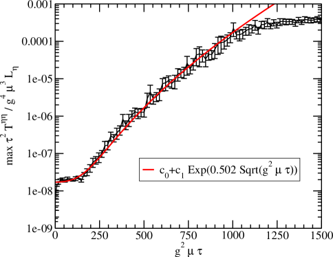
Fig. 1.: The maximum Fourier mode amplitudes of $\tau^{2}T^{\eta\eta}$ for $g^{2}\mu L=22.6$, $N_{\perp}=N_{\eta}=32$, $L_{\eta}=1.6$. Also shown is a best fit with a $\exp{\sqrt{\tau}}$ behavior. The flattening out of the data at late times is due to the non-Abelian interactions stopping the instability growth.

From Fig.1, one can see that from $g^{2}\mu\tau\approx 150$ onwards, there is rapid growth for which a best fit (up to times $g^{2}\mu\tau\sim 1000$) to the functional form $c_{0}+c_{1}\exp({\Gamma_{\rm fit}\tau^{c_{3}}})$ gives $\Gamma_{\rm fit}=0.502\pm 0.01$ for $c_{3}=0.5$; the coefficients $c_{0}$, $c_{1}$ are small numbers proportional to the initial seed.

In the presence of a Weibel instability, one expects $\tau^{2}\tilde{T}^{\eta\eta}$ to grow as $\exp(\sim\gamma\tau)$. For a system without expansion, $\gamma\sim m_{\infty}$ does not change as a function of $\tau$ and thus the instability manifests itself through modes growing as $\sim\exp(\tau)$. However, as argued in Ref.[9], the soft scale $m_{\infty}$ behaves as $m_{\infty}^{2}\sim 1/\tau$ in an expanding system. Therefore, the functional form of the growth is changed to $\exp(\sqrt{\tau})$. Our results confirm that this functional form is favored by a best fit to our data in Fig.1.

We can confirm this interpretation by also determining $m_{\infty}$ directly in our simulation. This is done by calculating the mass gap $\omega({\bf k_{\perp}}=0)$ of the gluon dispersion relation defined as [5],

$$\omega({\bf k}_{\perp})={1\over\tau}\sqrt{{{\rm Tr}\left[E_{i}({\bf k}_{\perp}E_{i}(-{\bf k}_{\perp})+\tau^{2}E_{\eta}({\bf k_{\perp}})E_{\eta}(-{\bf k}_{\perp})\right]\over{\rm Tr}\left[A_{i}({\bf k}_{\perp})A_{i}(-{\bf k}_{\perp})+{\tau}^{-2}A_{\eta}({\bf k}_{\perp})A_{\eta}(-{\bf k}_{\perp})\right]}},$$ (13)

which should be proportional to the soft scale $\omega({\bf k_{\perp}}=0)\sim m_{\infty}$. We find [6] $\omega({\bf k_{\perp}}=0)=\kappa_{0}\sqrt{g^{2}\mu/\tau}$, consistent with the expectation from [9, 14]. Interpreting $\omega({\bf k_{\perp}}=0)$ as the plasmon mass $\omega_{pl}$ we make use of the relation $\omega_{pl}^{2}=2/3m_{\infty}^{2}$  [6] to obtain the quantitative estimate $m_{\infty}=\kappa_{0}\sqrt{3g^{2}\mu/(2\tau)}$ for our simulation.

If we take the growth rate in the static case and make the change $\gamma_{stat}\tau\rightarrow\gamma(\tau)\tau$ with $\gamma(\tau)=m_{\infty}(\tau)/\sqrt{2}$ for the expanding system, we can define the “theoretical” growth rate $\Gamma_{\rm theory}\sqrt{g^{2}\mu\,\tau}=2\gamma\tau$. Obtaining $\Gamma_{\rm fit}$ by a best fit to the data (e.g. in Fig.1) for different values of $g^{2}\mu L$, we can compare this result to $\Gamma_{\rm theory}$, finding

$g^{2}\mu L$	$\Gamma_{\rm theory}=\sqrt{3}\,\kappa_{0}$	$\Gamma_{\rm fit}$
22.6	$0.526\pm 0.003$	$0.502\pm 0.01$
67.9	$0.447\pm 0.003$	$0.427\pm 0.01$
90.5	$0.49\pm 0.004$	$0.46\pm 0.04$

However, a consistent treatment would require that the growth rate in the expanding case is $exp(2\int_{0}^{\tau}d\tau^{\prime}\gamma(\tau^{\prime}))$; if we assume as previously that $\gamma(\tau^{\prime})=m_{\infty}(\tau)/\sqrt{2}$, one obtains an additional factor of 2 in the ratio of $\Gamma/\kappa_{0}$ relative to $\Gamma_{fit}$. Understanding this difference of a factor of $2$ requires a more careful study of the correspondence between the dynamics of expanding fields in our case and that in the static HTL case. In particular, it is important to investigate how $\omega_{pl}$ that we extract from the lattice relates to the plasmon frequency in Hard Thermal Loop simulations. Studies in this direction are in progress.

References

- [1] E. Iancu, R. Venugopalan, arXiv:hep-ph/0303204; in Hwa, R.C. (ed.) et al.: QGP3 (World Scientific Publishers).
- [2] L. V. Gribov, E. M. Levin and M. G. Ryskin, Phys. Rept. 100, 1 (1983); A. H. Mueller and J. w. Qiu, Nucl. Phys. B 268, 427 (1986).
- [3] L. McLerran, R. Venugopalan, Phys. Rev. D 49, 2233, 3352 (1994); ibid 50, 2225 (1994).
- [4] A. Kovner, L. D. McLerran and H. Weigert, Phys. Rev. D 52, 3809 (1995); ibid., 6231.
- [5] A. Krasnitz and R. Venugopalan, Nucl. Phys. B 557, 237 (1999); Phys. Rev. Lett. 84, 4309 (2000); 86, 1717 (2001); A. Krasnitz, Y. Nara and R. Venugopalan, Phys. Rev. Lett. 87, 192302 (2001); Nucl. Phys. A 717, 268 (2003); 727, 427 (2003); T. Lappi, Phys. Rev. C 67, 054903 (2003); arXiv:hep-ph/0505095.
- [6] P. Romatschke and R. Venugopalan, arXiv:hep-ph/0510121.
- [7] S. Mrówczyński, Phys. Lett. B 214, 587 (1988); Phys. Lett. B 314, 118 (1993); Phys. Lett. B 363, 26 (1997); J. Randrup, S. Mrówczyński, Phys. Rev. C 68, 034909 (2003).
- [8] P. Romatschke and M. Strickland, Phys. Rev. D 68, 036004 (2003); Phys. Rev. D 70, 116006 (2004); A. Rebhan, P. Romatschke and M. Strickland, Phys. Rev. Lett. 94, 102303 (2005).
- [9] P. Arnold, J. Lenaghan and G. D. Moore, JHEP 0308, 002 (2003); P. Arnold and J. Lenaghan, Phys. Rev. D70, 114007 (2004).
- [10] P. Arnold, J. Lenaghan, G. D. Moore and L. G. Yaffe, Phys. Rev. Lett. 94, 072302 (2005).
- [11] A. Dumitru and Y. Nara, Phys.Lett.B621, 89 (2005).
- [12] A. Rebhan, P. Romatschke, M. Strickland, Phys. Rev. Lett 94, 102303 (2005); JHEP 0509, 041 (2005). P. Arnold, G.D. Moore, L.G. Yaffe, Phys.Rev.D 72, 054003 (2005).
- [13] P. Romatschke and R. Venugopalan, in preparation.
- [14] R. Baier, A.H. Mueller, D. Schiff, D.T. Son, Phys. Lett. B 502, 51 (2001).