Charge screening effect in the hadron-quark mixed phase

Abstract

The Coulomb interaction effect and the surface effect are consistently taken into account in the hadron-quark mixed phase. These two finite-size effects greatly change the properties of the mixed phase and restrict its density region. In particular, the charge screening effect and the rearrangement of the charged particles are elucidated. Keeping the Gibbs conditions throughout the numerical procedure, we show the Maxwell construction effectively regain the physical meaning and the equation of state becomes similar to that given by the Maxwell construction.

1 Introduction

Deconfinement phase transition is believed to occur in hot and/or high-density matter, while its mechanism has not been well understood yet. Many authors have studied this transition by model calculations or first-principle calculations like lattice QCD[1]. Nowadays it is widely accepted that quark matter exists in hot and/or high-density region like inner core of neutron stars. Static and dynamic properties of quark matter have been actively studied theoretically for quark-gluon plasma (QGP), color superconductivity [2, 3] or magnetism [4, 5, 6]. Phenomenologically quark matter has been actively searched for in relativistic heavy-ion collisions (RHIC)[7], or in early universe and compact stars[8, 9].

Many theoretical calculations have suggested that the deconfinement phase transition should be of first order in low temperature and high density area[10, 11]. Therefore we assume first-order phase transition in this study. We, hereafter, consider the phase transition from nuclear matter to three-flavor quark matter in neutron-star matter for simplicity. If the deconfinement transition is of first order, we may expect the mixed phase during the transition. The hadron-quark mixed phase has been considered during the hadronization in RHIC[12, 13, 14] or the boundary between quark matter and hadron matter in neutron stars[15].

There is an issue about the mixed phase for the first-order phase transitions with more than one chemical potential[16]. We often use the Maxwell construction (MC) to derive the equation of state (EOS) in thermodynamic equilibrium, as in the water-vapor phase transition. In this case both phases consist of single particle species (${\rm H_{2}O}$). However, if many particle species participate in the phase transition as in neutron-star matter, MC is no more an appropriate method. Before Glendenning first pointed out [16], many people have applied MC to get EOS of the first-order phase transitions[17, 18, 19, 20] expected in neutron stars, such as pion or kaon condensation and the deconfinement transition.

For the deconfinement transition in neutron-star matter, we consider quark degrees of freedom as well as hadrons and leptons. Accordingly we must introduce many chemical potentials for particle species, but the independent ones in this case are reduced to two, i.e. baryon-number chemical potential $\mu_{\mathrm{B}}$ and charge chemical potential $\mu_{\mathrm{Q}}$, due to beta-equilibrium and total charge neutrality. They are nothing but the neutron and electron chemical potentials, $\mu_{n}$ and $\mu_{e}$, respectively. In the mixed-phase these chemical potentials should be spatially constant. When we naively apply MC to get EOS in thermodynamic equilibrium, we immediately notice that $\mu_{\mathrm{B}}$ is constant in the mixed-phase, while $\mu_{\mathrm{e}}$ is different in each phase because of the difference of the electron number in these phases. This is because MC uses EOS of bulk matter in each phase, which is of locally charge-neutral and uniform matter; many electrons are needed in hadron matter to cancel the positive charge of protons, while in quark matter total charge neutrality is almost fulfilled without electrons. Thus

$$\mu_{\mathrm{B}}^{\mathrm{Q}}=\mu_{\mathrm{B}}^{\mathrm{H}},\hskip 10.0pt\mu_{\mathrm{e}}^{\mathrm{Q}}\neq\mu_{\mathrm{e}}^{\mathrm{H}},$$ (1)

in MC, where superscripts “Q” and “H” denote the quark and hadron phase, respectively. Glendenning emphasized that we must use the Gibbs conditions (GC) in this case instead of MC, which relaxes the charge-neutrality condition to be globally satisfied as a whole, not locally in each phase [16]. GC imposes the following conditions,

$$\mu_{\mathrm{B}}^{\mathrm{Q}} =\mu_{\mathrm{B}}^{\mathrm{H}},\hskip 5.0pt\mu_{\mathrm{e}}^{\mathrm{Q}}=\mu_{\mathrm{e}}^{\mathrm{H}},$$

$$P^{\mathrm{Q}} =P^{\mathrm{H}},\hskip 5.0ptT^{\mathrm{Q}}=T^{\mathrm{H}}.$$ (2)

He demonstrated a wide region of the mixed phase, where two phases have a net charge but totally charge-neutral: EOS thus obtained, different from that given by MC, never exhibits a constant-pressure region. He simply considered the mixed phase consisting of two bulk matters separated by a sharp boundary without any surface tension and the Coulomb interaction, which we call “bulk Gibbs” for convenience.

“Bulk Gibbs” requires that each matter can have a net charge but total charge is neutral,

$$f_{V}\rho_{\mathrm{ch}}^{\mathrm{Q}}+(1-f_{V})\rho_{\mathrm{ch}}^{\mathrm{H}}=0,$$ (3)

where $f_{V}$ means the volume fraction of quark matter in the mixed phase and “$\rho_{\mathrm{ch}}^{\mathrm{Q,H}}$” means charge density in each matter. Figure 1 shows the phase diagram in the $\mu_{\mathrm{B}}$ - $\mu_{e}$ plane. We can see that there is a discontinuous jump in $\mu_{e}$ for the case of MC, while the curve given by “bulk Gibbs” smoothly connects uniform hadron matter and uniform quark matter; the mixed phase can appear in the wide $\mu_{\mathrm{B}}$ region in “bulk Gibbs”, in contrast with MC[21].

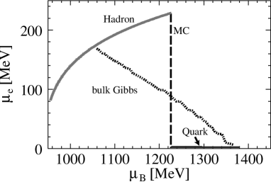
Figure 1: Phase diagram in the $\mu_{\mathrm{B}}-\mu_{\mathrm{e}}$ plane. There appears no region of the mixed phase by the calculation with MC, while a wide region of the mixed phase by the “bulk Gibbs” calculation.

However, this “bulk Gibbs” should be too simple to study the mixed phase, since we must consider non-uniform structures to be more realistic, instead of two bulk uniform matters; the mixed phase should have various geometrical structures, where both the number and charge densities are no more uniform. Then we have to take into account the finite-size effects like the surface and the Coulomb interaction energies. In this paper we study the structured mixed phase by treating the finite-size effects self-consistently. We show that the mixed phase should be narrow in the $\mu_{\mathrm{B}}$ space by the charge screening effect, and derive EOS for the deconfinement transition in neutron-star matter. We shall see it results in EOS being similar to the one given by MC. We also discuss the interplay of the Coulomb interaction effect and the surface effect in the context of the hadron-quark mixed phase. Preliminary results for the droplet case has been already reported in Ref.[28].

The plan of the paper is as follows. We briefly review the previous works in Sec. 2. Section 3 is devoted to our formalism and the numerical procedure. We show the results of our calculation and discuss the screening effect in Sec. 4. Finally, a summary and concluding remarks are given in Sec. 5.

2 Brief review of the previous works

Heiselberg et al. [22] studied a geometrical structure in the mixed phase: they considered spherical quark droplets embedded in hadron matter by including the surface and the Coulomb energies. They introduced the surface tension and treated its strength as a free parameter because the surface tension at the hadron-quark interface has not been clearly understood. They pointed out that if the surface tension parameter $\sigma$ is large ($\sigma\geq$ 90 MeV/fm²), the region of the mixed phase is largely limited or cannot exist. Subsequently Glendenning and Pei [15] have suggested the “crystalline structures of the mixed phase” which have some geometrical structures, “droplet”, “rod”, “slab”, “tube”, and “bubble”, assuming a small $\sigma$[15, 23].

The finite-size effects are obvious in these calculations by observing energies. We may consider only a single cell, by dividing the whole space into equivalent Wigner-Seitz cells: the cell size is denoted by $R_{W}$ and the size of the lump (droplet, rod, slab, tube or bubble) by $R$. Then the surface energy density is expressed in terms of the surface tension parameter $\sigma$ as

$$\epsilon_{\mathrm{S}}=\frac{f_{V}\sigma d}{R},$$ (4)

where $d$ denotes the dimensionality of each geometrical structure; $d=3$ for droplet and bubble, $d=2$ for rod and tube, and $d=1$ for slab. The Coulomb energy density reads

$$\epsilon_{\mathrm{C}} = 2\pi e^{2}\left(\rho_{\mathrm{ch}}^{\mathrm{H}}-\rho_{\mathrm{ch}}^{\mathrm{Q}}\right)^{2}R^{2}\Phi_{d}(f_{V})\hskip 5.0pt,$$ (5)

$$\Phi_{d}(f_{V}) \equiv \left[2(d-2)^{-1}\left(1-\frac{1}{2}df_{V}^{1-2/d}\right)+f_{V}\right]\left(d+2\right)^{-1},$$ (6)

where we simply assumed uniform density in each phase. When we minimize the sum of $\epsilon_{S}$ and $\epsilon_{C}$ with respect to the size $R$ for a given volume fraction $f_{V}$, we can get the well known relation,

$$\epsilon_{S}=2\epsilon_{C}.$$ (7)

This implies that an optimal size of the lump is determined by the balance of these finite-size effects. Eventually we can express the size-dependent energy density besides the bulk energy density [22]:

$$\epsilon^{(d)}_{\mathrm{C}}+\epsilon^{(d)}_{\mathrm{S}}=3f_{V}d\left(\frac{\pi\sigma^{2}\left(\rho_{\mathrm{ch}}^{\mathrm{H}}-\rho_{\mathrm{ch}}^{\mathrm{Q}}\right)^{2}\Phi_{d}(f_{V})}{2d}\right)^{1/3}.$$ (8)

Thus we can calculate the energy of any geometrically structured mixed phase with (8) by changing the parameter $d$. Many authors have taken this treatment for the mixed phase[15, 21, 22]. Note that the energy sum in Eq. (8) becomes larger as the surface tension gets stronger, while the relation Eq.(7) is always kept.

However, this treatment is not a self-consistent, but a perturbative one, since the charge screening effect for the Coulomb potential or the rearrangement of charged-particles in the presence of the Coulomb interaction is completely discarded. We shall see that the Coulomb potential is never weak in the mixed phase, and thereby this treatment overestimates the Coulomb energy. The charge screening effect is included only if we introduce the Coulomb potential and consistently solve the Poisson equation with other equations of motion for charged particles. Consequently it is a highly non-perturbative effect. Norsen and Reddy[24] have studied the Debye screening effect in the context of kaon condensation to see a large change of the charged-particle densities like kaons and protons. Maruyama et al. have numerically studied it in the context of liquid-gas phase transition at subnuclear densities [25], where nuclear pastas can be regarded as geometrical structures in the mixed phase. Subsequently, they have also studied kaon condensation at high-densities [26], where we have seen that kaonic pastas appear in the mixed phase. Through these works we have figured out the role of the Debye screening in the mixed phase. We have also studied the interplay of the Coulomb effect and the surface effect.

Voskresensky et al. [27] explicitly studied the Debye screening effect for a few geometrical structures of the hadron-quark mixed phase. They have shown that the optimal value of the size of the structure cannot be obtained due to the charge screening even if the surface tension is not so strong. They called it as mechanical instability. It occurs because the Coulomb energy density is suppressed at larger size than the Debye screening length (cf. Eq. (34)). They also suggested that the properties of the mixed phase become very similar to those given by MC, if the charge screening effectively works. They also noted that the apparent violation of the Gibbs condition (Eq. (1)) can be remedied by including the Coulomb potential in a gauge-invariant way: the number of the charged particles is given by a gauge invariant combination of the chemical potential and the Coulomb potential, and thereby the number can be different in each phase for a constant charge chemical potential if the the Coulomb potential takes different values in both phases. However, they used a linear approximation to solve the Poisson equation analytically.

If the Coulomb interaction effect is so important, it would be important to study it without recourse to any approximation. In this paper we numerically study the charge screening effect on the structured mixed phase during the deconfinement transition in neutron-star matter in a self-consistent way. Actually we shall see importance of non-linear effects included in the Poisson equation.

3 Self-consistent calculation

3.1 Thermodynamic potential

We consider the geometrically structured mixed phase (SMP) where one phase is embedded in the other phase with a certain geometrical form.

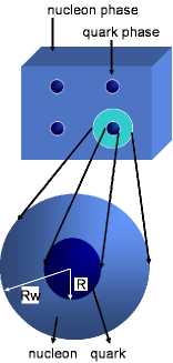
Figure 2: Wigner-Seitz approximation for the droplet case. $R$ is the droplet radius and $R_{\mathrm{W}}$ the cell radius.

We divide the whole space into equivalent charge-neutral Wigner-Seitz cells with a size $R_{W}$ and a size of embedded phase $R$ as illustrated in Fig. 2. Quark phase consists of u, d, s quarks and electron. Hadron phase consists of proton, neutron and electron. We incorporate the MIT Bag model and assume the sharp boundary at the hadron-quark interface. We use density functional theory (DFT) and incorporate local density approximation (LDA) [29, 30].

We consider total thermodynamic potential ($\Omega_{\mathrm{total}}$) which consists of the hadron, quark and electron and the Coulomb interaction contributions:

$$\Omega_{\mathrm{total}}=\Omega_{\mathrm{hadron}}+\Omega_{\mathrm{quark}}+\Omega_{\mathrm{em}},$$ (9)

where we summarize the contributions of electrons and the Coulomb interaction as $\Omega_{\mathrm{em}}$ because they are present in both phases.

We briefly present the expressions of thermodynamic potentials. The details of the derivation of the expressions are given in Ref.[31].

First, the Coulomb interaction energy is expressed in terms of particle densities,

$$E_{V}=\frac{1}{2}\sum_{i,j}\int d^{3}rd^{3}r^{\prime}\frac{Q_{i}\rho_{i}(\vec{r})Q_{j}\rho_{j}(\vec{r}^{\prime})}{\left|\vec{r}-\vec{r}^{\prime}\right|},$$ (10)

where $i=u,d,s,p,n,e$ with $Q_{i}$ being the particle charge ($Q=-e<0$ for the electron). Accordingly the Coulomb potential is defined as

$$V(\vec{r})=-\sum_{i}\int d^{3}r^{\prime}\frac{eQ_{i}\rho_{i}(\vec{r}^{\prime})}{\left|\vec{r}-\vec{r}^{\prime}\right|}+V_{0},$$ (11)

where $V_{0}$ is an arbitrary constant representing the gauge degree of freedom. We fix the gauge by a condition $V(R_{W})=0$ in this paper (see Sec. 2.2). Operating a Laplacian $\nabla^{2}$ on the Coulomb potential $V(\vec{r})$, we automatically derive the Poisson equation.

Therefore, the electron contribution and the Coulomb interaction energy (in both phases) are expressed as

$$\Omega_{\mathrm{em}}\!\! = \!\!\int\!d\vec{r}\Biggl{[}-\frac{1}{8\pi e^{2}}\left(\nabla V(\vec{r})\right)^{2}+\epsilon_{e}(\rho_{e}(\vec{r}))-\mu_{e}\rho_{e}(\vec{r})+V(\vec{r})\rho_{e}(\vec{r})\Biggr{]}$$ (12)

$$= \!\int\!d\vec{r}\left[-\frac{1}{8\pi e^{2}}\left(\nabla V(\vec{r})\right)^{2}\!-\!\frac{\left(V(\vec{r})\!-\!\mu_{e}\right)^{4}}{12\pi^{2}}\!\right],$$

where $\epsilon_{e}(\rho_{e}(\vec{r}))=\frac{\left(3\pi^{2}\rho_{e}(\vec{r})\right)^{\frac{4}{3}}}{4\pi^{2}}$ is the kinetic energy density of electron.

Secondly, in the quark phase, u and d quarks are treated as massless particles and only s quark massive one, $m_{s}=150$ MeV. The kinetic energy of quark of flavor $f$ is simply expressed as[32]

$$\epsilon_{f\mathrm{kin}}=\frac{3}{8\pi^{2}}m_{f}^{4}\left[x_{f}\eta_{f}\left(2x_{f}^{2}+1\right)-\ln\left(x_{f}+\eta_{f}\right)\right],$$ (13)

where $m_{f}$ is the quark mass, $x_{f}=p_{\mathrm{F}f}(\vec{r})/m_{f}$ with Fermi momentum $p_{\mathrm{F}f}(\vec{r})=(\pi^{2}\rho_{f}(\vec{r}))^{\frac{1}{3}}$ and $\eta_{f}=\sqrt{1+x^{2}_{f}}$.

For the interaction energy, we take into account the leading order contribution coming from the one-gluon exchange interaction. Since the contribution from the Hartree term disappears due to the traceless property of the Gell-Mann matrix ($\lambda$), the leading order contribution only comes from the Fock term,

$$\epsilon_{f\mathrm{Fock}}=-\frac{\alpha_{\mathrm{c}}}{\pi^{3}}m_{f}^{4}\left\{x_{f}^{4}-\frac{3}{2}\left[x_{f}\eta_{f}-\ln\left(x_{f}+\eta_{f}\right)\right]^{2}\right\}.$$ (14)

Including this interaction, the quark contribution to the thermodynamic potential is expressed as

$$\Omega_{\mathrm{quark}}=\Omega_{\mathrm{u}}+\Omega_{\mathrm{d}}+\Omega_{\mathrm{s}}+\int d\vec{r}B,$$ (15)

$$\Omega_{f} = \int\!d\vec{r}\left[\epsilon_{f}(\rho_{f}(\vec{r}))-\mu_{f}\rho_{f}(\vec{r})-N_{i}V(\vec{r})\rho_{f}(\vec{r})\right],\hskip 10.0ptN_{i}=\frac{Q_{i}}{e},$$

where, the energy density $\epsilon_{f}(\rho_{f}(\vec{r}))$ stands for $\epsilon_{f\mathrm{kin}}+\epsilon_{f\mathrm{Fock}}$ of $f$ quark, and $B$ is the Bag constant. The Bag constant is taken as 120 MeV/fm³, and the QCD fine structure constant as $\alpha_{\mathrm{c}}=0.4$, which are also used by Heiselberg et al. [22] and in the previous work[27].

Thirdly, we consider the hadron contribution. The thermodynamic potential for the non-relativistic nucleons becomes

$$\Omega_{\mathrm{hadron}}=E_{N}-\sum_{a=p,n}\mu_{a}\int d\vec{r}\rho_{a}(\vec{r})-\int d\vec{r}\,V(\vec{r})\rho_{\mathrm{p}}(\vec{r}),$$ (16)

where $E_{N}$ is the energy of the nucleons,

$$E_{N}=\int d\vec{r}\left[\sum_{a=p,n}\frac{3}{10m}\left(3\pi^{2}\right)^{\frac{2}{3}}\rho^{\frac{5}{3}}_{a}(\vec{r})+\epsilon_{\mathrm{pot}}\left(\rho_{\mathrm{p}}(\vec{r}),\rho_{\mathrm{n}}(\vec{r})\right)\right].$$ (17)

Here we use the effective potential $\epsilon_{\mathrm{pot}}(\rho_{\mathrm{p}}(\vec{r}),\rho_{\mathrm{n}}(\vec{r}))$ parametrized by the local densities for simplicity,

$$\epsilon_{\mathrm{pot}}(\vec{r}) = S_{0}\frac{\left(\rho_{\mathrm{n}}(\vec{r})-\rho_{\mathrm{p}}(\vec{r})\right)}{\rho_{0}(\vec{r})}+\left(\rho_{\mathrm{n}}(\vec{r})+\rho_{\mathrm{p}}(\vec{r})\right)\epsilon_{\mathrm{bind}}$$ (18)

$$+ K_{0}\frac{\left(\rho_{\mathrm{n}}(\vec{r})+\rho_{\mathrm{p}}(\vec{r})\right)}{18}\left(\frac{\rho_{\mathrm{n}}(\vec{r})+\rho_{\mathrm{p}}}{\rho_{0}}-1\right)^{2}$$

$$+ C_{\mathrm{sat}}\left(\rho_{\mathrm{n}}(\vec{r})+\rho_{\mathrm{p}}(\vec{r})\right)\left(\frac{\rho_{\mathrm{n}}(\vec{r})+\rho_{\mathrm{p}}(\vec{r})}{\rho_{0}}-1\right),$$

where $S_{0}$, $K_{0}$, $\epsilon_{\mathrm{bind}}$, and $C_{\mathrm{sat}}$ are adjustable parameters to reproduce the saturation properties of nuclear matter[27]. We consider beta equilibrium at the hadron-quark interface as well as in each phase:

$$\mu_{\mathrm{u}}+\mu_{\mathrm{e}}=\mu_{\mathrm{d}},$$

$$\mu_{\mathrm{d}}=\mu_{\mathrm{s}},$$

$$\mu_{\mathrm{p}}+\mu_{\mathrm{e}}=\mu_{\mathrm{n}}\equiv\mu_{\mathrm{B}},$$

$$\mu_{\mathrm{n}}=\mu_{\mathrm{u}}+2\mu_{\mathrm{d}},$$

$$\mu_{\mathrm{p}}=2\mu_{\mathrm{u}}+\mu_{\mathrm{d}}.$$ (19)

The last relation can be derived from other four relations, so that there are left four independent conditions for chemical equilibrium.

We get the equations of motion from $\frac{\delta\Omega_{\mathrm{total}}}{\delta\phi_{i}}=0$ ( $\phi_{i}=\rho_{u}(\vec{r}),\rho_{d}(\vec{r}),\rho_{s}(\vec{r}),$ $\rho_{p}(\vec{r}),\rho_{n}(\vec{r}),\rho_{e}(\vec{r}),V(\vec{r})$ ): The Poisson equation then reads

$$\nabla^{2}V(\vec{r})\!\!=\!\!4\pi e^{2}\left[\left(\frac{2}{3}\rho_{u}(\vec{r})-\frac{1}{3}\rho_{d}(\vec{r})-\frac{1}{3}\rho_{s}(\vec{r})\right)+\rho_{\mathrm{p}}(\vec{r})-\rho_{e}(\vec{r})\right].$$ (20)

Other equations of motion give nothing but the expressions of the chemical potentials,

$$\mu_{i}=\frac{\delta E_{\mathrm{kin+str}}}{\delta\rho_{i}(\vec{r})}-N_{i}V(\vec{r}),$$ (21)

where $\displaystyle E_{\mathrm{kin+str}}=\sum_{i=u,d,s,e}\int d\vec{r}\epsilon_{i}+E_{N}$. Then quark chemical potentials are expressed as

$$\mu_{\mathrm{u}} = \left(1+\frac{2\alpha_{\mathrm{c}}}{3\pi}\right)\pi^{\frac{2}{3}}\rho_{\mathrm{u}}^{\frac{1}{3}}(\vec{r})-\frac{2}{3}V(\vec{r})$$ (22)

$$\mu_{\mathrm{d}} = \left(1+\frac{2\alpha_{\mathrm{c}}}{3\pi}\right)\pi^{\frac{2}{3}}\rho_{\mathrm{d}}^{\frac{1}{3}}(\vec{r})+\frac{1}{3}V(\vec{r})$$ (23)

$$\mu_{\mathrm{s}} = \epsilon_{{\mathrm{Fs}}}(\vec{r})+\frac{2\alpha_{\mathrm{c}}}{3\pi}\left[p_{\mathrm{Fs}}(\vec{r})-3\frac{m_{\mathrm{s}}^{2}}{\epsilon_{\mathrm{Fs}}(\vec{r})}\ln\left(\frac{\epsilon_{\mathrm{Fs}}(\vec{r})+p_{\mathrm{Fs}}(\vec{r})}{m_{\mathrm{s}}}\right)\right]+\frac{1}{3}V(\vec{r}),$$

with $\epsilon_{\mathrm{Fs}}(\vec{r})=\sqrt{m_{\mathrm{s}}^{2}+p_{\mathrm{Fs}}^{2}(\vec{r})}$. On the other hand chemical potentials of nucleons and electrons are

$$\mu_{\mathrm{n}} = \frac{p_{\mathrm{Fn}}^{2}}{2m}+\frac{2S_{0}\left(\rho_{n}(\vec{r})-\rho_{\mathrm{p}}(\vec{r})\right)}{\rho_{0}}+\epsilon_{\mathrm{bind}}$$ (25)

$$+ \frac{K_{0}}{6}\left(\frac{\rho_{\mathrm{n}}(\vec{r})\!+\!\rho_{\mathrm{p}}(\vec{r})}{\rho_{0}}-1\right)^{2}+\frac{K_{0}}{9}\left(\frac{\rho_{\mathrm{n}}(\vec{r})+\rho_{\mathrm{p}}(\vec{r})}{\rho_{0}}-1\right)$$

$$+ 2C_{\mathrm{sat}}\frac{\rho_{\mathrm{n}}(\vec{r})+\rho_{\mathrm{p}}(\vec{r})}{\rho_{0}}-C_{\mathrm{sat}}$$

$$\mu_{\mathrm{p}} = \mu_{\mathrm{n}}-\frac{p_{\mathrm{Fn}}^{2}(\vec{r})}{2m}+\frac{p_{\mathrm{Fp}}^{2}(\vec{r})}{2m}-\frac{4S_{0}\left(\rho_{\mathrm{B}}-2\rho_{\mathrm{p}}(\vec{r})\right)^{2}}{\rho_{0}}-V(\vec{r})$$

$$\mu_{e} = \left(3\pi^{2}\rho_{e}(\vec{r})\right)^{\frac{1}{3}}+V(\vec{r}).$$ (26)

We solve these equations of motion under GC. Important point is that the Coulomb potential $V(\vec{r})$ is included in each expression in a proper way. The Coulomb potential is the function of charged-particle densities, and in turn densities are functions of the Coulomb potential. As a result, the Poisson equation becomes highly non-linear. Since it should be difficult to solve them analytically, we numerically solve them without any approximation.

Once the geometrical structure is concerned, we have to take into account the surface tension as well at the interface of the hadron and quark phases. It may be connected with the confining mechanism and unfortunately we have no definite idea about how to incorporate it. Actually many authors have treated its strength as a free parameter and seen how the results are changed by its value[15, 22, 21]. Here we also follow this manner by introducing the surface tension parameter $\sigma$ to simulate the surface effect. One might be afraid that the surface tension will be modified once the Coulomb interaction is explicitly introduced. However, such modification might be rather small, as inferred from the previous result[26].

Note that we have to determine now eight variables, i.e., six chemical potentials, $\mu_{\mathrm{u}}$, $\mu_{\mathrm{d}}$, $\mu_{\mathrm{s}}$, $\mu_{\mathrm{p}}$, $\mu_{\mathrm{n}}$, $\mu_{\mathrm{e}}$, and radii $R$ and $R_{W}$. First, we fix $R$ and $R_{W}$. Here we have four conditions due to $\beta$ equilibrium (19). Therefore, once two chemical potentials $\mu_{\mathrm{B}}$ and $\mu_{\mathrm{e}}$ are given, we can determine other four chemical potentials, $\mu_{\mathrm{u}}$, $\mu_{\mathrm{d}}$, $\mu_{\mathrm{s}}$ and $\mu_{\mathrm{p}}$. Next, we determine $\mu_{\mathrm{e}}$ by the global charge neutrality condition:

$$f_{V}\rho_{\mathrm{ch}}^{\mathrm{Q}}+(1-f_{V})\rho_{\mathrm{ch}}^{\mathrm{H}}=0,$$ (27)

where the volume fraction $f_{V}=\left(\frac{R}{R_{W}}\right)^{d}$, and $d$ denotes the dimensionality of each geometrical structure. At this point $f_{V}$ is still fixed.

The pressure coming from the surface tension is given by

$$P_{\sigma}=\sigma\frac{dS}{dV_{\rm Q}},$$ (28)

where $S$ is the area of the surface and $V_{\rm Q}$ is the volume of the quark phase. Then we find the optimal value of $R$ ($R_{W}$ is fixed and thereby $f_{V}$ is changed by $R$) by using one of GC;

$$P^{\mathrm{Q}}=P^{\mathrm{H}}+P_{\sigma}.$$ (29)

The pressure in each phase $P^{\mathrm{Q(H)}}$ is given by the thermodynamic relation: $P^{\mathrm{Q(H)}}=-\Omega_{\mathrm{Q(H)}}/V_{\mathrm{Q(H)}}$, where $\Omega_{\mathrm{Q(H)}}$ is the thermodynamic potential in each phase and given by adding electron and the Coulomb interaction contributions to $\Omega_{\mathrm{quak(hadron)}}$ in Eqs. (15) and (16). Finally, we determine $R_{W}$ by minimizing thermodynamic potential. Therefore once $\mu_{\mathrm{B}}$ is given, all other values $\mu_{i}$ ($i=u,d,s,p,e$) and $R$, $R_{W}$ can be obtained.

Note that we keep GC throughout the numerical procedure. We will see later how the mixed phase would be changed by including finite-size effects keeping GC completely. Although MC is not rigidly correct as we have seen in Sec. 1, our results will show a similar behavior to those by MC as a result of including the finite-size effects.

In numerical calculation, every point inside the cell is represented by a grid point (the number of grid points $N_{\mathrm{grid}}\approx 100$). Equations of motion are solved by a relaxation method for a given baryon-number chemical potential under constraints of the global charge neutrality.

3.2 Proper treatment of the Coulomb interaction

With the Coulomb potential (11) and thermodynamic potentials (9), the gauge invariance of our treatment can easily be seen as follows: varying the expression of chemical potentials (21) with respect to the Coulomb potential $V(\vec{r})$, as is shown in the previous work[27], we have

$$A_{ij}\frac{\partial\rho_{j}}{\partial V}=N_{i},\hskip 10.0pt\hskip 5.0ptA_{ij}B_{jk}=\delta_{ik},$$ (30)

where matrices $A$ and $B$ are defined as

$$A_{ij}\equiv\frac{\delta^{2}E_{\mathrm{kin+str}}}{\delta\rho_{i}\delta\rho_{j}}\hskip 10.0ptB_{ij}\equiv\frac{\partial\rho_{i}}{\partial\mu_{j}}.$$ (31)

From these equations, the gauge-invariance relation follows,

$$\frac{\partial\rho_{i}}{\partial V}=N_{j}\frac{\partial\rho_{j}}{\partial\mu_{i}}.$$ (32)

We can understand that chemical potential is gauge variant from this relation. When the Coulomb potential is shifted by a constant value, $V(\vec{r})\Longrightarrow V({\vec{r}})-V_{0}$, the charge chemical potential should be also shifted as $\mu_{i}\Longrightarrow\mu_{i}+N_{i}V_{0}$. To take into account the Coulomb interaction, we have to include $V(\vec{r})$ in the gauge invariant way like in Eq. (21). Note that the phase diagram in the $\mu_{\mathrm{B}}-\mu_{\mathrm{e}}$ plane (see ,e.g., Fig. 1) is not well-defined, since the charge chemical potential $\mu_{e}$ is not gauge invariant by itself.

4 Numerical results

We show the thermodynamic potential in Figs. 4 and 4. In uniform matter, hadron phase is thermodynamically favorable for $\mu_{\mathrm{B}}<1225$ MeV and quark phase for $\mu_{\mathrm{B}}>1225$. Therefore we plot $\delta\omega$, difference of the thermodynamic potential density between the mixed phase and each uniform matter:

$$\delta\omega=\begin{cases}\omega_{\mathrm{total}}-\omega^{\mathrm{uniform}}_{\mathrm{H}}\quad\mu_{\mathrm{B}}\leq 1225\mathrm{MeV},\\ \omega_{\mathrm{total}}-\omega^{\mathrm{uniform}}_{\mathrm{Q}}\quad\mu_{\mathrm{B}}\geq 1225\mathrm{MeV},\end{cases}$$ (33)

where $\omega_{\mathrm{total}}=\Omega_{\mathrm{total}}/V_{W}$, etc. There we also depict two results for comparison: one is given by the “bulk Gibbs” calculation, where the finite-size effects are completely discarded. The other is the thermodynamic potential given by a perturbative treatment of the Coulomb interaction, which is denoted by “no Coulomb”; discarding the Coulomb potential $V(\vec{r})$, we solve the equations of motion to get density profiles, then evaluate the Coulomb interaction energy by using the density profiles thus determined. We can see the screening effects by comparing this “no Coulomb” calculation with the self-consistent one denoted by “screening”. $\delta\omega$ given by MC appears as a point denoted by a circle in Figs. 4 and 4 where two conditions, $P^{\mathrm{Q}}=P^{\mathrm{H}}$ and $\mu_{\mathrm{B}}^{\mathrm{Q}}=\mu_{\mathrm{B}}^{\mathrm{H}}$, are satisfied. On the other hand the mixed phase derived from “bulk Gibbs” appears in a wide region of $\mu_{\mathrm{B}}$. Therefore, if the region of the mixed phase becomes narrower, it signals that the properties of the mixed phase become close to those of MC. One may clearly see that $\omega_{\mathrm{total}}$ becomes close to that given by MC due to the finite-size effects, the effects of the surface tension and the Coulomb interaction.

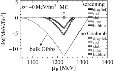
Figure 3: Difference of the thermodynamic potential density as a function of baryon-number chemical potential $\mu_{\mathrm{B}}$ for $\sigma=40$ MeV/fm². If $\delta\omega$ is negative, the mixed phase is a thermodynamically favorable state. MC determines one point of phase transition in uniform matter, denoted as a circle in the $\mu_{B}$-$\delta\omega$ plane.

Figure 4: Same as Fig. 3 for $\sigma=60$ MeV/fm². The negative $\delta\omega$ region is narrower than the $\sigma=40$ MeV/fm² case.

The large increase of $\delta\omega$ from the “bulk Gibbs” curve comes from the effects of the surface tension and the Coulomb potential. Since the surface tension parameter is introduced by hand, we must carefully study the effects of the surface tension and the Coulomb interaction, separately. From the difference between the result given by “no Coulomb” and that by “bulk Gibbs”, we can roughly say that about $2/3$ of the increase comes from the effect of the surface tension and $1/3$ from the Coulomb interaction (see Eq. (7)).

Comparing the result of self-consistent calculation with that of “no Coulomb”, we can see that the change of energy caused by the screening effect is not so large, but still the same order of magnitude as that given by the surface effect.

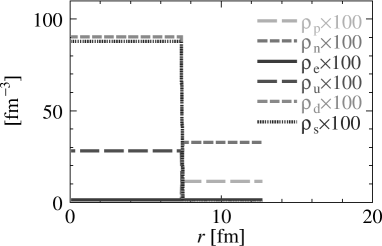
Figure 5: Density profiles in the droplet phase given by “no Coulomb” for $\mu_{B}=1189$ MeV and $\sigma=60$ MeV/fm². They are uniform in each phase. $R=7.2$ fm and $R_{W}=12.8$ fm.

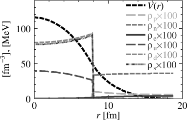
Figure 6: Density profiles and the Coulomb potential given by the self-consistent calculation for the same parameter set as Fig. 5. $R=7.7$ fm and $R_{W}=18.9$ fm.

If the surface tension is stronger, the relative importance of the screening effect becomes smaller and the effect of the surface tension becomes more dominant, as is seen in Fig. 4.

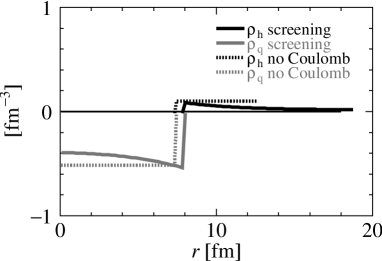
Figure 7: Local-charge densities for the “no Coulomb” case and the case of the self-consistent with the screening effect. For “no Coulomb”, charge density of each phase is constant over the region. The absolute value of the charge density is larger than that given by the self-consistent calculation in each phase. In the hadron phase, the charge density becomes almost vanished near the cell boundary $r=R_{W}$.

To be more realistic we have to take into account the modification of the surface tension as the structure size changes. Though we cannot clearly say how the surface tension is affected, we may infer from the previous study that it is not so large. Although the charge screening has not so large effects on bulk properties of the matter, we shall see that it is remarkable for the charged particles to change the properties of the mixed phase.

The screening effect induces the rearrangement of the charged particles. We can see this screening effect by comparing Fig. 6 with Fig. 6. The quark phase is negatively charged and the hadron phase is positively charged. The negatively charged particles in the quark phase such as d, s, e and the positively charged particle in the hadron phase p are attracted toward the boundary. On the contrary the positively charged particle in the quark phase u and negatively charged particle in the hadron phase e are repelled from the boundary. The charge screening effect also reduces the net charge in each phase. In Fig. 7, we show the local charge densities of the two cases shown in Figs. 6 and 6. The change of the number of charged particles due to the screening is as follows: In the quark phase, the numbers of $d$ and $s$ quarks and electrons decrease, while the number of $u$ quark increases. In the hadron phase, on the other hand, the proton number should decrease and the electron number should increase. Consequently the local charge decreases in the both phases. In Fig. 7 we can see that the core region of the droplet tends to be charge-neutral and near the boundary of the Wigner-Seitz cell is almost charge-neutral.

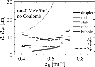
Figure 8: Lump and cell radii given by the “no Coulomb” calculation. The Debye screening length is also depicted for comparison. $R$ is thick-solid line and $R_{W}$ is thick-dashed line. We can see the size of the structure becomes less than the Debye screening length.

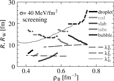
Figure 9: Same as Fig. 8 given by the self-consistent calculation with the screening effect. The size of the structure becomes larger than that given by “no Coulomb”, and consequently exceeds the Debye screening length.

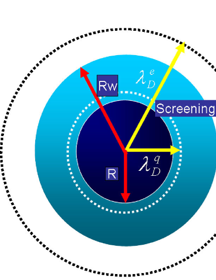
Figure 10: Schematic graphs of the droplet size and the Debye screening length. Right figure shows the case of the self-consistent calculation with the screening effect and left figure “no Coulomb”.

In Figs.  9 and 9 we present the lump and cell radii for each density. As we have shown in the previous paper[27], the Coulomb energy is suppressed for larger $R$ by the screening effect. The $R$ dependence of the total thermodynamic potential comes from the contributions of the surface tension and the Coulomb interaction: the optimal radius giving the minimum of the thermodynamic potential is then determined by the balance between two contributions, since the former gives a decreasing function, while the latter an increasing one. If the Coulomb energy is suppressed, the minimum of the thermodynamic potential is shifted to larger radius. As a result the size of the embedded phase ($R$) and the cell size ($R_{W}$) become large. In Ref. [27] they demonstrated that the minimum disappears for a large value of the surface tension parameter: the structure becomes mechanically unstable in this case. We cannot show it directly in our framework because such unstable solutions are automatically excluded during the numerical procedure, while we can see its tendency in Figs. 9 and 9: $R$ and $R_{W}$ get larger by the screening effect.

We also see the relation between the size of the geometrical structure and the Debye screening length. The Debye screening length appears in the linearized Poisson equation and is then given as

$$\left(\lambda^{q}_{D}\right)^{-2}\!\!=\!4\pi\sum_{f}Q_{f}\!\left(\frac{\partial\langle\rho_{f}^{\mathrm{ch}}\rangle}{\partial\mu_{f}}\right),\hskip 5.0pt\left(\lambda^{p}_{D}\right)^{-2}\!\!=\!4\pi Q_{p}\!\left(\frac{\partial\langle\rho_{p}^{\mathrm{ch}}\rangle}{\partial\mu_{p}}\right),\hskip 5.0pt\left(\lambda^{e}_{D}\right)^{-2}\!\!=\!4\pi Q_{e}\!\left(\frac{\partial\langle\rho_{e}^{\mathrm{ch}}\rangle}{\partial\mu_{e}}\right),$$ (34)

where $\langle\rho_{f}^{\mathrm{ch}}\rangle$ stands for the averaged density in quark phase, $\langle\rho_{p}^{\mathrm{ch}}\rangle$ is proton number averaged density in the hadron phase and $\langle\rho_{e}^{\mathrm{ch}}\rangle$ is the electron charge density averaged inside the cell. It gives a rough measure for the screening effect: At a distance larger than the Debye screening length, the Coulomb interaction is effectively suppressed.

In Fig. 9 we show sizes of geometrical structure for “no Coulomb” case. If we ignore the screening effect, the size of the embedded phase is comparable or smaller than the corresponding quark Debye screening length $\lambda_{D}^{q}$ (Fig. 10). This may mean that the Debye screening is not so important. Actually, many authors have neglected the screening effect due to this argument[22, 21]. In Fig. 9, however, we see that the size of the embedded phase can be larger than $\lambda_{D}^{q}$ (Fig. 10) in the self-consistent calculation. We can also see the similar situation about $R_{W}$ and $\lambda_{D}^{e}$. This means that the screening has important effects in this mixed phase. We cannot expect such a effect without solving the Poisson equation because of the non-linearity. We show the EOS in Figs. 12 and 12. The pressure of the mixed phase becomes similar to that given by MC due to the screening effect.

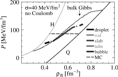
Figure 11: Pressure as a function of baryon-number density given by the “no Coulomb” calculation for $\sigma=40$MeV/fm². The results given by “bulk Gibbs” and MC are also presented for comparison.

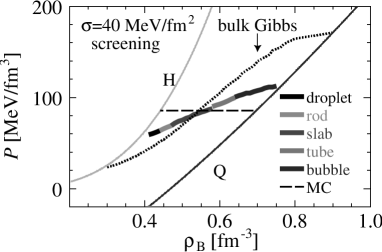
Figure 12: Same as Fig. 12 given by the self-consistent calculation with the screening effect.

We have used a fixed surface tension parameter in the present study. Surface tension is a very difficult problem because it should be self-consistent with the two phases of matter, quark and hadron. Lattice QCD, based on the first principle, would be the most reliable theory. It predicts that the surface tension can be 10-100 MeV/fm²[33, 34]. Although this range is for high temperature, our choice is within it. Moreover, other model calculations of the surface tension[35, 36, 37, 38] are similar to our choice. Although we cannot conclude that MC is perfectly correct, we can say that the results obtained by the “no Coulomb” calculation, which many authors have used, have to be checked again taking into account the finite-size effects.

Let us consider some implication of these results for neutron star phenomena. Glendenning[15] suggested many SMP appear in the core region by using “bulk Gibbs”: the mixed phase should appear for several kilometers. However we can say that the region of SMP should be narrow in the $\mu_{\mathrm{B}}$ space and EOS is more similar to that of MC due to the finite-size effects. These results correspond to recent other calculations. Bejger et al. [39] have examined the relation between the mixed phase and glitch phenomena, and shown that the mixed phase should be narrow if the glitch is generated by the mixed phase in the inner core. On the other hand the gravitational wave asks for density discontinuity in the core region[40]. These studies support our result.

5 Summary and concluding remarks

We have numerically studied the charge screening effect in the hadron-quark mixed phase, by fully including the non-linear effects in the Poisson equation. Comparing the results with those given by “no Coulomb” calculation, we have elucidated the screening effect. The density profiles of the charged particles are much modified by the screening effect, while the thermodynamic potential is not so much affected; the charge rearrangement induced by the screening effect tends to make the net charge smaller in each phase. Consequently the system tends to be locally charge-neutral, which suggests that MC is effectively justified even if it is thermodynamically incorrect. In this context, it would be interesting to refer to the work by Heiselberg [41], who studied the screening effect on a quark droplet (strangelet) in the vacuum, and suggested the importance of the rearrangement of charged particles.

We have seen that thermodynamic quantities such as thermodynamic potential and pressure become close to those derived from MC by the screening effect, which also suggests that MC is effectively justified due to the screening effect. As another case of more than one chemical potential system, kaon condensation has been also studied[25] and the results are similar to those in the present study. Thus the importance of the screening effect should be a common feature for the first-order phase transitions in high-density matter.

We have included the surface tension at the hadron-quark interface, while its definite value is not clear at present. There are also many estimations for the surface tension at the hadron-quark interface in lattice QCD [33, 34], in shell-model calculations [35, 36, 37] and in model calculations based on the dual-Ginzburg Landau theory [38]. Our parameter is in that reasonable range.

We have considered some implications of our results for neutron star phenomena. The screening effect would restrict the allowed SMP region in neutron stars, in contrast with a wide region given by “bulk Gibbs”[15, 23]. It could be said that they should change the bulk property of neutron stars, especially the structure of the core region.

Compact stars have the strong magnetic field and its origin is not well understood. One possibility is that it comes from quark matter in the core[4, 5, 6]. Therefore it should be interesting to include the magnetic field contribution in our formalism.

We have assumed zero temperature here. It would be much interesting to include the finite-temperature effect. Then it is possible to draw the phase diagram in the $\mu_{\mathrm{B}}$ - $T$ plane and we can study the properties of the deconfinement phase transition; our study may be extended to treat the mixed phase to appear during the hadronization of QGP in the nucleus-nucleus collisions and supernova explosions.

In this study we have used a simple model for quark matter to figure out the finite-size effects in the SMP. However, it has been suggested that the color superconductivity would be a ground state of quark matter [2, 21]. Hence we will include it in a further study. The hadron phase should be also treated more realistically; for example, we should include the hyperons or kaons in hadron matter. In the recent studies the mixed phase has been also studied [42, 43] in the context of various phases in the color superconducting phase.

References

- [1] For review, D. H. Rischke, Prog. Part. Nucl. Phys. 52 (2004) 197; J. Macher and J. Schaffner-Bielich, Eur. J. Phys. 26 (2005) 341 and references therein.
- [2] M. Alford, K. Rajagopal and F. Wilczek, Nucl. Phys. B 64 (1999) 443, D. Bailin and A. Love, Phys. Rep. 107 (1984) 325. As resent reviews, M. Alford, hep-ph/0102047; K. Rajagopal and F. Wilczek, hep-ph/0011333
- [3] M. Alford and S. Reddy, Phys. Rev. D 67 (2003) 074024
- [4] T. Tatsumi, T. Maruyama and E. Nakano, Prog. Theor. Phys. Suppl. 153 (2004) 190
- [5] E. Nakano, T. Maruyama and T. Tatsumi, Phys. Rev. D 68 (2003) 105001
- [6] T. Tatsumi, Phys. Lett. B 489 (2000) 280
- [7] K. Adcox et al. (PHENIX collaboration), Phys. Rev. Lett. 88 (2002) 022301; C. Adler et al. (STAR collaboration), Phys. Rev. Lett. 90 (2003) 082302
- [8] J. Madsen, Lect. Notes Phys. 516 (1999) 162
- [9] K. S. Cheng, Z. G. Dai and T. Lu, Int. Mod. Phys. D7 (1998) 139
- [10] R. D. Pisalski and F. Wilczek, Phys. Rev. Lett. 29 (1984) 338
- [11] R. V. Gavai, J. Potvin and S. Sanielevici, Phys. Rev. Lett. 58 (1987) 2519
- [12] Y. A. Terasov, Phys. Rev. C 70 (2004) 054904
- [13] S. Pratt and S. Pal, Phys. Rev. C 71 (2005) 014905
- [14] J. M. Peters and K. L. Haglin J. Phys. G: Nucl. Part. Phys.31 (2005) 49
- [15] N. K. Glendenning and S. Pei, Phys. Rev. C D52 (1995) 2250
- [16] N. K. Glendenning, Phys. Rev. D D46 (1992) 1274; hys. Rep. 342 (2001) 393.
- [17] W. Weise, and G. E. Brown, Phys. Lett. B 58 (1975) 300
- [18] A. B. Migdal, A. I. Chernoustan and I. N. Mishustin, Phys. Lett. B 83 (1979) 158
- [19] J. Ellis, J. Kapusta and K. A. Olive, Nucl. Phys. B 348 (1991) 345
- [20] A. Rosenhauer, E. F. Staubo, L. P. Csernai, T. Øvergård, and E. Østgaad, Nucl. Phys. A 540 (1992) 630
- [21] M. Alford, K. Rajagopal, S. Reddy, and F. Wilczek, Phys. Rev. D 64 (2001) 074017
- [22] H. Heiselberg, C. J. Pethick and E. F. Staubo, Phys. Rev. Lett. 70 (1993) 1355
- [23] N. K. Glendenning, Compact stars, Springer 2000.
- [24] T. Norsen and S. Reddy, Phys. Rev. C. 63 (2001) 065804
- [25] Toshiki Maruyama, T. Tatsumi, D. N. Voskresensky, T. Tanigawa and S. Chiba, Nucl. Phys. A 749 (2005) 186c; Phys. Rev C 72 (2005) 015802
- [26] Toshiki Maruyama, T. Tatsumi, D. N. Voskresensky, T. Tanigawa, T. Endo and S. Chiba, nucl-th/0505063
- [27] D. N. Voskresensky, M. Yasuhira and T. Tatsumi, Phys. Lett. B541 (2002) 93, ; Nucl. Phys. A723 (2003) 291; T. Tatsumi, M. Yasuhira and D. N. Voskresensky, Nucl. Phys. A718 (2003) 359c; T. Tatsumi and D. N. Voskresensky, nucl-th/0312114.
- [28] T. Endo, Toshiki Maruyama, S. Chiba and T. Tatsumi, Nucl. Phys. A 749 (2005) 333c
- [29] R. G. Parr and W. Yang, Density-Functional Theory of atoms and molecules, Oxford Univ. Press, 1989.
- [30] E. K. U. Gross and R. M. Dreizler, Density functional theory, Plenum Press (1995)
- [31] T. Endo, Toshiki Maruyama, S. Chiba and T. Tatsumi, hep-ph/0502216
- [32] R. Tamagaki and T. Tatsumi, Prog. Theor. Phys. Suppl. 112 (1993) 277
- [33] K. Kajantie, L. Kärkäinen, and K. Rummukainen, Nucl. Phys. B357 (1991) 693
- [34] S. Huang, J. Potvion, C. Rebbi and S. Sanielevici, Phys. Rev. D 43 (1991) 2056
- [35] J. Madsen, Phys. Rev. D 46 (1992) 329
- [36] J. Madsen, Phys. Rev. Lett. 70 (1993) 391
- [37] M. S. Berger and R. L. Jaffe, Phys. Rev. C 35 (1987) 213
- [38] H. Monden, H. Ichie, H. Suganuma and H. Toki, Phys. Rev. C 57 (1998) 2564
- [39] M. Bejger, P. Haensel and J. L. Zdunik, Mon. Not. Roy. Astron. Soc. 359 (2005) 699
- [40] G. Miniutti, J. A. Pons, E. Berti, L. Gualtieri, V. Ferrari, Mon. Not. Roy. Astron. Soc. 338 (2003) 389
- [41] H. Heiselberg, Phys.Rev.D. 48 (1993) 1418
- [42] I. Shovkovy, M. Hanauske and M. Huang, Phys. Rev. D 67 (2003) 103004
- [43] S. Reddy and G. Rupak, nucl-th/0405054