$D_{sJ}^{+}(2317)\to D_{s}^{+}\pi^{0}$ decay width

Abstract

We use the QCD sum rules to analize the hadronic decay $D_{sJ}^{+}(2317)\to D_{s}^{+}\pi^{0}$, in the hypotesis that the $D_{sJ}^{+}(2317)$ can be identified as a four-quark state. We use a diquak-antidiquark current and work to the order of $m_{s}$ in full QCD, without relying on $1/m_{c}$ expansion. We find that the partial decay width of the hadronic isospin violating mode is proportional to the isovector quark condensate, $\langle 0|\bar{d}d-\bar{u}u|0\rangle$. The estimated partial decay width is of the order of 6 keV.

The strange-charmed mesons $D_{sJ}^{+}(2317)$ and $D_{sJ}^{+}(2460)$ with spin parity $0^{+}$, $1^{+}$ babar ; cleo ; belle1 ; focus are lighter than the prediction of the very successful quark model for the charmed mesons god . One interpretation is that this is evidence for a chiral symmetry where the mass gap between the $0^{-}$ and $1^{-}$ states equates the mass gap between the $0^{+}$ and $1^{+}$ states bar . Other interpretations are related with the underlying structure of these mesons, which has been extensively debated. They have been interpreted as conventional $c\bar{s}$ states dhlz ; bali ; ukqcd ; ht ; nari ; dnp ; cf ; god2 ; fr ; whz , two-meson molecular state bcl ; szc , $D-K$- mixing br or four-quark states ch ; tera ; mppr ; blmnn ; kioh ; bpp ; dmi ; hte .

Because of their low masses, these two states are lower than the $DK$ and $D^{*}K$ thresholds. Therefore, their strong decays must proceed through isospin violating effects. There have been some discussions of their decays within the quark model bar ; cf ; god2 ; fr ; ch and QCD sum rules whz . In all these studies but god2 , the isospin violating effects were considered through the $\eta-\pi^{0}$ mixing. However, if these mesons are considered as four-quark states, in a QCD sum rule calculation, the isospin violating effects can be introduced through the mass and quark condensate difference between the $u$ and $d$ quarks.

In a recent calculation blmnn the scalar-isoscalar meson $D_{sJ}^{+}(2317)$ were considered as a $S$-wave bound state of a diquark-antidiquark pair. As suggested in ref. jawil , the diquark was taken to be a spin zero colour anti-triplet. The corresponding interpolating field is:

$$j_{S} = {\epsilon_{abc}\epsilon_{dec}\over\sqrt{2}}\left[(u_{a}^{T}C\gamma_{5}c_{b})(\bar{u}_{d}\gamma_{5}C\bar{s}_{e}^{T})+(d_{a}^{T}C\gamma_{5}c_{b})(\bar{d}_{d}\gamma_{5}C\bar{s}_{e}^{T})\right],$$ (1)

where $a,~{}b,~{}c,~{}...$ are colour indices and $C$ is the charge conjugation matrix. In ref. blmnn , using the QCD sum rule (QCDSR) formalism svz ; rry ; io1 , it was shown that it is possible to reproduce the experimental mass of the meson $D_{sJ}^{+}(2317)$ using this four-quark state picture. Here, we extend the calculation done in ref. blmnn to study the vertex associated with the decay $D_{sJ}^{+}(2317)\to D_{s}^{+}\pi^{0}$.

The QCDSR calculation for the vertex, $D_{sJ}^{+}(2317)D_{s}^{+}\pi^{0}$, centers around the three-point function given by

$$\Gamma_{\mu}(p,p^{\prime},q)=\int d^{4}xd^{4}y~{}e^{ip^{\prime}.x}~{}e^{iq.y}\langle 0|T[j_{D_{s}}(x)j_{5\mu}^{\pi^{0}}(y)j^{\dagger}_{S}(0)]|0\rangle,$$ (2)

where $p=p^{\prime}+q$ and the interpolating fields for the pion and $D_{s}$ mesons are given by:

$$j_{5\mu}^{\pi^{0}}={1\over\sqrt{2}}(\bar{u}_{a}\gamma_{\mu}\gamma_{5}u_{a}-\bar{d}_{a}\gamma_{\mu}\gamma_{5}d_{a}),\,\;\;\;j_{D_{s}}=i\bar{s}_{a}\gamma_{5}c_{a}.$$ (3)

The fundamental assumption of the QCD sum rule approach is the principle of duality. Specifically, we assume that there is an interval over which the above vertex function may be equivalently described at both, the quark level and at the hadron level. Therefore, the underlying procedure of the QCD sum rule technique is the following: on one hand we calculate the vertex function at the quark level in terms of quark and gluon fields. On the other hand, the vertex function is calculated at the hadronic level introducing hadron characteristics such as masses and coupling constants. At the quark level the complex structure of the QCD vacuum leads us to employ the Wilson’s operator product expansion (OPE). The calculation of the phenomenological side proceeds by inserting intermediate states for $D_{s}$, $\pi^{0}$ and $D_{sJ}$, and by using the definitions:

$$\langle 0|j_{5\mu}^{\pi^{0}}|\pi^{0}(q)\rangle=iq_{\mu}F_{\pi},\;\;\;\;\langle 0|j_{D_{s}}|D_{s}(p^{\prime})\rangle={m_{D_{s}}^{2}f_{D_{s}}\over m_{c}+m_{s}},\;\;\;\;\langle 0|j_{D_{sJ}}|D_{sJ}(p)\rangle=\lambda_{S}.$$ (4)

We obtain the following relation:

$$\Gamma_{\mu}^{phen}(p,p^{\prime},q)={\lambda_{S}m_{D_{s}}^{2}f_{D_{s}}F_{\pi}~{}g_{D_{sJ}D_{s}\pi}\over(m_{c}+m_{s})(p^{2}-m_{D_{sJ}}^{2})({p^{\prime}}^{2}-m_{D_{s}}^{2})(q^{2}-m_{\pi}^{2})}~{}~{}q_{\mu}+\mbox{continuum contribution}\;,$$ (5)

where the coupling constant $g_{D_{sJ}D_{s}\pi}$ is defined by the on-mass-shell matrix element

$$\langle D_{s}\pi|D_{sJ}\rangle=g_{D_{sJ}D_{s}\pi}.$$ (6)

The continuum contribution in Eq.(5) contains the contributions of all possible excited states.

For the light scalar mesons, considered as diquark-antidiquark states, the study of their vertices functions using the QCD sum rule approach at the pion pole rry ; nari ; nari2 ; brann , was done in ref.sca . In Table I we show the results obtained for the different vertices studied in ref. sca , as well as the experimental values.

Table I: Numerical results for the coupling constants

vertex	$g(\nobreak\,\mbox{GeV})$	$g^{exp}(\nobreak\,\mbox{GeV})$
$\sigma\pi^{+}\pi^{-}$	$3.1\pm 0.5$	$2.6\pm 0.2$
$\kappa K^{+}\pi^{-}$	$3.6\pm 0.3$	$4.5\pm 0.4$
$f_{0}K^{+}K^{-}$	$1.6\pm 0.1$
$f_{0}\pi^{+}\pi^{-}$	$0.47\pm 0.05$	$1.6\pm 0.8$

From Table I we see that, although not exactly in between the experimental error bars, the hadronic couplings determined from the QCD sum rule calculation are consistent with existing experimental data. The biggest discrepancy is for $g_{f_{0}\pi^{+}\pi^{-}}$ and this can be understood since the $f_{0}\to\pi^{+}\pi^{-}$ decay is mediated by gluon exchange and, therefore, probably in this case $\alpha_{s}$ corrections, which were not considered, could play an important role.

Here, we follow ref. sca and work at the pion pole. The main reason for working at the pion pole is that the matrix element in Eq.(6) defines the coupling constant only at the pion pole. For $q^{2}\neq 0$ one would have to replace $g_{D_{sJ}D_{s}\pi}$, in Eq.(6), by the form factor $g_{D_{sJ}D_{s}\pi}(q^{2})$ and, therefore, one would have to deal with the complications associated with the extrapolation of the form factor bclnn ; dfnn . The pion pole method consists in neglecting the pion mass in the denominator of Eq. (5) and working at $q^{2}=0$. In the OPE side one singles out the leading terms in the operator product expansion of Eq.(2) that match the $1/q^{2}$ term. In the phenomenological side, in the structure ${q_{\mu}\over q^{2}}$ we get:

$$\Gamma^{phen}(p^{2},{p^{\prime}}^{2})={\lambda_{S}m_{D_{s}}^{2}f_{D_{s}}F_{\pi}~{}g_{D_{sJ}D_{s}\pi}\over(m_{c}+m_{s})(p^{2}-m_{D_{sJ}}^{2})({p^{\prime}}^{2}-m_{D_{s}}^{2})}+\int_{m_{c}^{2}}^{\infty}{\rho_{cont}(p^{2},u)\over u-{p^{\prime}}^{2}}~{}du.$$ (7)

In Eq.(7), $\rho_{cont}(p^{2},u)$, gives the continuum contributions, which can be parametrized as $\rho_{cont}(p^{2},u)={b(u)\over s_{0}-p^{2}}\Theta(u-u_{0})$ ennr ; io2 , with $s_{0}$ and $u_{0}$ being the continuum thresholds for $D_{sJ}$ and $D_{s}$ respectively. Since we are working at $q^{2}=0$, we take the limit $p^{2}={p^{\prime}}^{2}$ and we apply the Borel transformation to $p^{2}\rightarrow M^{2}$ to get:

$$\Gamma^{phen}(M^{2})={\lambda_{S}m_{D_{s}}^{2}f_{D_{s}}F_{\pi}~{}g_{D_{sJ}D_{s}\pi}\over(m_{c}+m_{s})(m_{D_{sJ}}^{2}-m_{D_{s}}^{2})}\left(e^{-m_{D_{s}}^{2}/M^{2}}-e^{-m_{D_{sJ}}^{2}/M^{2}}\right)+A~{}e^{-s_{0}/M^{2}}+\int_{u_{0}}^{\infty}\rho_{cc}(u)~{}e^{-u/M^{2}}du,$$ (8)

where

$$A=-\int_{u_{0}}^{\infty}{b(u)\over(s_{0}-u)}~{}du,\;\;\mbox{and }\;\;\rho_{cc}(u)={b(u)\over(s_{0}-u)},$$ (9)

stands for the pole-continuum transitions and pure continuum contributions. For simplicity, one assumes that the pure continuum contribution to the spectral density, $\rho_{cc}(u)$, is given by the result obtained in the OPE side. Asymptotic freedom ensures that equivalence for sufficiently large $u$. Therefore, one uses the ansatz: $\rho_{cc}(u)=\rho_{OPE}(u)$. In Eq.(8), $A$ is a parameter which, together with $g_{D_{sJ}D_{s}\pi}$, have to be determined by the sum rule.

In the OPE side we work at leading order and deal with the strange quark as a light one and consider the diagrams up to order $m_{s}$. To keep the charm quark mass finite, we use the momentum-space expression for the charm quark propagator. We calculate the light quark part of the correlation function in the coordinate-space, which is then Fourier transformed to the momentum space in $D$ dimensions. The resulting light-quark part is combined with the charm-quark part before it is dimensionally regularized at $D=4$. Singling out the leading terms proportional to $q_{\mu}/q^{2}$, we can write the Borel transform of the correlation function in the OPE side in terms of a dispersion relation:

$$\Gamma^{OPE}(M^{2})=\int_{m_{c}^{2}}^{\infty}\rho_{OPE}(u)~{}e^{-u/M^{2}}du\;,$$ (10)

where the spectral density, $\rho_{OPE}$, is given by the imaginary part of the correlation function. Transferring the pure continuum contribution to the OPE side, the sum rule for the coupling constant, up to dimension 7, is given by:

$$C~{}\left(e^{-m_{D_{s}}^{2}/M^{2}}-e^{-m_{D_{sJ}}^{2}/M^{2}}\right)+A~{}e^{-s_{0}/M^{2}}=\gamma\langle\bar{q}q\rangle\left[{1\over 2^{4}\pi^{2}}\int_{m_{c}^{2}}^{u_{0}}du~{}e^{-u/M^{2}}u\left(1-{m_{c}^{2}\over u}\right)^{2}\right.$$

$$\left.+{m_{c}m_{s}\over 8\pi^{2}}\int_{m_{c}^{2}}^{u_{0}}du~{}e^{-u/M^{2}}\left(1-{m_{c}^{2}\over u}\right)-{m_{c}\langle\bar{s}s\rangle\over 6}e^{-m_{c}^{2}/M^{2}}+{m_{s}\langle\bar{s}s\rangle\over 12}e^{-m_{c}^{2}/M^{2}}\left(1+{m_{c}^{2}\over M^{2}}\right)\right],$$ (11)

with

$$C={\lambda_{S}m_{D_{s}}^{2}f_{D_{s}}F_{\pi}\over(m_{c}+m_{s})(m_{D_{sJ}}^{2}-m_{D_{s}}^{2})}~{}g_{D_{sJ}D_{s}\pi}.$$ (12)

In Eq.(11), $\gamma$ measures the isospin symmetry breaking in the quark condensate:

$$\gamma={\langle 0|\bar{d}d-\bar{u}u|0\rangle\over\langle 0|\bar{u}u|0\rangle},$$ (13)

and is the source of nonperturbative isospin violation in the OPE of the vertex function. The value of $\gamma$ has been estimated in a variety of approaches nari2 ; gale ; jim , with results varying over almost one order of magnitude: $-1\times 10^{-2}\leq\gamma\leq-2\times 10^{-3}$. A more recent calculation kms gives a bigger (in module) value: $\gamma=-2.6\times 10^{-2}$.

In the numerical analysis of the sum rules, the values used for the meson masses, quark masses and condensates are: $m_{D_{sJ}}=2.317~{}\nobreak\,\mbox{GeV}$, $m_{D_{s}}=1.968~{}\nobreak\,\mbox{GeV}$, $m_{s}=0.13\,\nobreak\,\mbox{GeV}$, $m_{c}=1.2\,\nobreak\,\mbox{GeV}$, $\langle\bar{q}q\rangle=\,-(0.23)^{3}\,\nobreak\,\mbox{GeV}^{3}$, $\langle\overline{s}s\rangle\,=0.8\langle\bar{q}q\rangle$. For the meson decay constants we use $F_{\pi}=\sqrt{2}~{}93\nobreak\,\mbox{MeV}$ and $f_{D_{s}}=0.22~{}\nobreak\,\mbox{GeV}$ (obtained using $u_{0}=6~{}\nobreak\,\mbox{GeV}^{2}$ beni ). For the current meson coupling, $\lambda_{S}$, defined in Eq.(4) we are going to use the result obtained from the two-point function in ref. blmnn . Considering $2.6\leq\sqrt{s_{0}}\leq 2.8~{}\nobreak\,\mbox{GeV}$ we get $\lambda_{s}=(2.9\pm 0.3)\times 10^{-3}~{}\nobreak\,\mbox{GeV}^{5}$.

In Fig. 1 we show, through the dots, the right-hand side (RHS) of Eq.(11), for $u_{0}=6~{}\nobreak\,\mbox{GeV}^{2}$ and $\gamma=-1\times 10^{-2}$ jim , as a function of the Borel mass. We use the same Borel window as defined in ref.blmnn .

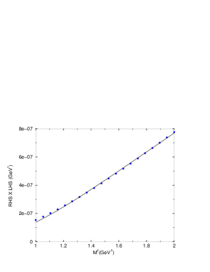
Figure 1: Dots: the RHS of Eq.(11), as a function of the Borel mass. The solid line gives the fit of the QCDSR results through the LHS of Eq.(11).

To determine $g_{D_{sJ}D_{s}\pi}$ we fit the QCDSR results with the analytical expression in the left-hand side (LHS) of Eq.(11):

$$C\left(e^{-m_{D_{s}}^{2}/M^{2}}-e^{-m_{D_{sJ}}^{2}/M^{2}}\right)+A~{}e^{-s_{0}/M^{2}},$$ (14)

and we get (using $\sqrt{s_{0}}=2.7\nobreak\,\mbox{GeV}$): $C=8.34\times 10^{-6}~{}\nobreak\,\mbox{GeV}^{7}$ and $A=6.96\times 10^{-6}~{}\nobreak\,\mbox{GeV}^{7}$. Using the definition of $C$ in Eq.(12) and $\lambda_{S}=2.9\times 10^{-3}~{}\nobreak\,\mbox{GeV}^{5}$ (the value obtained for $\sqrt{s_{0}}=2.7\nobreak\,\mbox{GeV}$) we get $g_{D_{sJ}D_{s}\pi}=50~{}\nobreak\,\mbox{MeV}$. Allowing $s_{0}$ to vary in the interval $2.6\leq\sqrt{s_{0}}\leq 2.8~{}\nobreak\,\mbox{GeV}$, the corresponding varyation obtained for the coupling constant is $45~{}\nobreak\,\mbox{MeV}\leq g_{D_{sJ}D_{s}\pi}\leq 55~{}\nobreak\,\mbox{MeV}$.

Fixing $\sqrt{s_{0}}=2.7\nobreak\,\mbox{GeV}$ and varying the quark condensate, the charm quark and the strange quark masses in the intervals: $-(0.24)^{3}\leq\langle\bar{q}q\rangle\leq-(0.22)^{3}\,\nobreak\,\mbox{GeV}^{3}$, $1.1\leq m_{c}\leq 1.3\nobreak\,\mbox{GeV}$ and $0.11\leq m_{s}\leq 0.15\nobreak\,\mbox{GeV}$, we get results for the coupling constant still between the lower and upper limits given above. However, varying the value of $\gamma$ form $-1\times 10^{-2}$ to the more recent value given in kms : $\gamma=-2.6\times 10^{-2}$, and keeping the other parameters fixed we get $g_{D_{sJ}D_{s}\pi}=130~{}\nobreak\,\mbox{MeV}$. On the other hand, if we use the smallest (in module) value allowed for $\gamma$: $\gamma=-2.\times 10^{-3}$, we get $g_{D_{sJ}D_{s}\pi}=10~{}\nobreak\,\mbox{MeV}$. Therefore, the biggest source of uncertainty in our calculation is the value of $\gamma$. In all cases considered here, the quality of the fit between the LHS and the RHS of Eq.(11) is similar to the one shown in Fig.1.

The coupling constant, $g_{D_{sJ}D_{s}\pi}$, is related with the partial decay width through the relation:

$$\Gamma(D_{sJ}^{+}(2317)\rightarrow D_{s}^{+}\pi^{0})={1\over 16\pi m_{D_{sJ}}^{3}}g_{D_{sJ}D_{s}\pi}^{2}\sqrt{\lambda(m_{D_{sJ}}^{2},m_{D_{s}}^{2},m_{\pi}^{2})},$$ (15)

where $\lambda(a,b,c)=a^{2}+b^{2}+c^{2}-2ab-2ac-2bc$. Considering $\gamma=-1\times 10^{-2}$, which was the value found in jim to be consistent with the neutron-proton mass difference in a QCDSR calculation, and allowing $\langle\bar{q}q\rangle$, $m_{c},~{}m_{s}$ and $s_{0}$ to vary in the ranges discussed above we get:

$$\Gamma(D_{sJ}^{+}(2317)\rightarrow D_{s}^{+}\pi^{0})=(6\pm 2)\nobreak\,\mbox{keV}.$$ (16)

However, it is important to state that, if the value for $\gamma$ found in ref.kms proves to be correct, then the partial decay width could be as large as $\Gamma(D_{sJ}^{+}(2317)\rightarrow D_{s}^{+}\pi^{0})\sim 40\nobreak\,\mbox{keV}$, in agreement with the QCDSR calculation done in ref.whz , where the meson $D_{sJ}^{+}(2317)$ is considered as a ordinary $c\bar{s}$ state.

In Table II we show the partial decay width obtained by different theoretical groups. The first five calculations assume a $c\bar{s}$ picture for $D_{sJ}^{+}(2317)$, while the last two assume a four-quark picture for it.

Table II: The decay width $\Gamma(D_{sJ}^{+}(2317)\rightarrow D_{s}^{+}\pi^{0})$ from various theoretical approaches.
ref. bar cf god2 fr whz ch this work $\Gamma$ (keV) $~{}21.5~{}$ $~{}7\pm 1~{}$ $~{}\sim 10~{}$ $~{}16~{}$ $~{}39\pm 5~{}$ $~{}10-100~{}$ $~{}6\pm 2~{}$

From the results in Table II we see that we can not get a definitive answer about the structure of the $D_{sJ}(2317)$ meson from its strong decay width, since in both pictures: ordinary $c\bar{s}$ or four-quark states, different approachs can give results varying from a few keV to a hundred keV.

We have presented a QCD sum rule study of the vertex function associated with the strong decay $D_{sJ}^{+}(2317)\rightarrow D_{s}^{+}\pi^{0}$, where the $D_{sJ}^{+}(2317)$ meson was considered as diquark-antidiquark state. We found that the source of isospin violation in our calculation is the parameter $\gamma={\langle 0|\bar{d}d-\bar{u}u|0\rangle\over\langle 0|\bar{u}u|0\rangle}$, which measures the isospin symmetry breaking in the quark condensate. Since, in our approach, the partial decay width is directly proportional to $\gamma^{2}$, and since there is a large uncertainty in the value of $\gamma$, considering $\gamma$ in the range $-2.6\times 10^{-2}\leq\gamma\leq-2\times 10^{-3}$ we get the partial decay width in the range $0.2\nobreak\,\mbox{keV}\leq\Gamma(D_{sJ}^{+}(2317)\rightarrow D_{s}^{+}\pi^{0})\leq 40\nobreak\,\mbox{keV}$. However, from other QCDSR calculation, we believe that the value of $\gamma$ is $\sim-1\times 10^{-2}$, which gives the result shown in Eq.(16).

As a final remark we would like to point out that if, instead of using a isoscalar current, we have used a isovector current for $D_{sJ}(2317)$ (as suggested in ref. hte ), the difference in Eq.(11) would be a factor 2 in the place of $\gamma$. In this case the decay would be isospin allowed and the partial width would be $\sim 230~{}\nobreak\,\mbox{MeV}$, much bigger than the experimental upper limit to the total width $\Gamma\sim 5~{}\nobreak\,\mbox{MeV}$.

Acknowledgements: I would like to thank F.S. Navarra and I. Bediaga for fruitful discussions. This work has been supported by CNPq and FAPESP.

References

(1) BABAR Coll., B. Auber et al., Phys. Rev. Lett.
90, 242001 (2003); Phys. Rev. D69, 031101 (2004).
(2) CLEO Coll., D. Besson et al., Phys. Rev. D68,
032002 (2003).
(3) BELLE Coll., P. Krokovny et al., Phys. Rev. Lett.
91, 262002 (2003).
(4) FOCUS Coll., E.W. Vaandering, hep-ex/0406044.
(5) S. Godfrey and N. Isgur, Phys. Rev. D32, 189 (1985);
S. Godfrey and R. Kokoshi, Phys. Rev. D43, 1679 (1991).
(6) W. Bardeen, E. Eichten and C. Hill, Phys. Rev. D68,
054024 (2003).
(7) Y.-B. Dai, C.-S. Huang, C. Liu and S.-L. Zhu,
Phys. Rev. D68, 114011 (2003).
(8) G.S. Bali, Phys. Rev. D68, 071501(R) (2003).
(9) A. Dougall, R.D. Kenway, C.M. Maynard and C. Mc-Neile,
Phys. Lett. B569, 41 (2003).
(10) A. Hayashigaki and K. Terasaki, hep-ph/0411285.
(11) S. Narison, Phys. Lett. B605, 319 (2005).
(12) A. Deandrea, G. Nardulli and A. Polosa, Phys. Rev. D68,
097501 (2003).
(13) P. Colangelo and F. De Fazio, Phys. Lett. B570, 180
(2003).
(14) S. Godfrey, Phys. Lett. B568, 254 (2003).
(15) Fayyazuddin and Riazuddin, Phys. Rev. D69, 114008 (2004).
(16) W. Wei, P.-Z. Huang and S.-L. Zhu, hep-ph/0510039.
(17) T. Barnes, F.E. Close and H.J. Lipkin, Phys. Rev. D68,
054006 (2003).
(18) A.P. Szczepaniak, Phys. Lett. B567, 23 (2003).
(19) E. van Beveren and G. Rupp, Phys. Rev. Lett. 91,
012003 (2003).
(20) H.-Y. Cheng and W.-S. Hou, Phys. Lett. B566, 193 (2003).
(21) K. Terasaki, Phys. Rev. D68, 011501(R) (2003).
(22) L. Maiani, F. Piccinini, A.D. Polosa, V. Riquer,
Phys. Rev. D71, 014028 (2005).
(23) M.E. Bracco et al., Phys. Lett. B624, 217 (2005).
(24) H. Kim and Y. Oh, hep-ph/0508251.
(25) T. Browder, S. Pakvasa and A.A. Petrov, Phys. Lett.
B578, 365 (2004).
(26) U. Dmitrasinovic, Phys. Rev. D70, 096011 (2004);
Phys. Rev. Lett. 94, 162002 (2005).
(27) A. Hayashigaki and K. Terasaki, hep-ph/0410393.
(28) R.L. Jaffe and F. Wilczek, Phys. Rev. Lett. 91,
232003 (2003).
(29) M.A. Shifman, A.I. and Vainshtein and V.I. Zakharov,
Nucl. Phys. B147, 385 (1979).
(30) L.J. Reinders, H. Rubinstein and S. Yazaky, Phys. Rep.
127, 1 (1985).
(31) B. L. Ioffe, Nucl. Phys. B188, 317 (1981);
B191, 591(E) (1981).
(32) S. Narison, Spectral Sum Rules, World Scientific Lecture
Notes in Physics 26.
(33) M.E. Bracco, F.S. Navarra, M. Nielsen,
Phys. Lett. B454, 346 (1999).
(34) T.V. Brito, F.S. Navarra, M. Nielsen, M.E. Bracco, Phys. Lett.
B608, 69 (2005).
(35) M.E. Bracco et al., Phys. Lett. B521, 1 (2001).
(36) H.G. Dosch, E.M. Ferreira, F.S. Navarra and M. Nielsen, Phys.
Rev. D65, 114002 (2002).
(37) B. L. Ioffe and A.V. Smilga, Nucl. Phys. B232, 109
(1984).
(38) M. Eidemúller et al., Phys. Rev. D72, 034003
(2005).
(39) J. Gasser, H. Leutwyler, Nucl. Phys. . B250, 465 (1985).
(40) X. Jin, M. Nielsen, J. Pasupathy, Phys. Rev. D51, 3688
(1995); H. Forkel, M. Nielsen, Phys. Rev. D55, 1471 (1997), and
references therein.
(41) H.-C. Kim, M.M. Musakhanov, M. Siddikov, hep-ph/0508211.
(42) I. Bediaga, M. Nielsen, Phys. Rev. D68,
036001 (2003).