Small-x QCD effects in forward-jet and Mueller-Navelet jet production

Abstract

We investigate small$-x$ QCD effects in forward-jet production in deep inelastic scattering in the kinematic regime where the virtuality of the photon and the transverse momentum of the jet are two hard scales of about the same magnitude. We show that the data from HERA published by the H1 and ZEUS collaborations are well described by leading-logarithmic BFKL predictions. Parametrizations containing saturation effects expected to be relevant at higher energies also compare well to the present data. We extend our analysis to Mueller-Navelet jets at the LHC and discuss to what extent this observable could test these small$-x$ effects and help distinguishing between the different descriptions.

I Introduction

The Regge limit of perturbative QCD comes about when the centre-of-mass energy in a collision is much bigger than the fixed hard scales of the problem. In this limit usually called the small$-x$ regime, parton densities inside the projectiles grow with increasing energy, leading to the growth of the scattering amplitudes. As long as the densities are not too high, this growth is described by the Balitsky-Fadin-Kuraev-Lipatov (BFKL) equation bfkl that resums the leading logarithms. As the parton density becomes higher and the scattering amplitudes approach the unitarity limit, one enters a regime called saturation glr ; glr+ ; mv ; jimwlk where the BFKL evolution breaks down and parton densities saturate.

In the past years, as colliders started to explore the small$-x$ regime, proposals were made to test the relevance of the BFKL equation at the available energies. In this paper we concentrate on two of the proposed measurements: forward jets dis in deep inelastic scattering (DIS) and Mueller-Navelet jets mnj in hadron-hadron collisions. Forward-jet production is a process in which the virtual photon interacts with the proton and a jet is detected in the forward direction of the proton. The virtuality of the photon and the squared transverse momentum of the jet are hard scales of about the same magnitude. In the case of Mueller-Navelet jets, a proton interacts with another proton or antiproton and a jet is detected in each of the two forward directions; the transverse momenta of the jets are as well hard scales of about the same magnitude. If the total energy in the photon-proton (for forward jets) or proton-proton (for Mueller-Navelet jets) collision is large enough, these processes feature the kinematics corresponding to the Regge limit.

The description of forward jets with fixed-order perturbative QCD in the Bjorken limit amounts in the following. Large logarithms coming from the strong ordering between the soft proton scale and the hard forward-jet scale are resummed using the Dokshitzer-Gribov-Lipatov-Altarelli-Parisi (DGLAP) evolution equation dglap and the hard cross-section is computed at fixed order in the coupling constant. In the small$-x$ regime, due to the extra ordering between the total energy and the hard scales, other large logarithms arise and should be resummed within the hard cross-section itself. In other words, the inclusion of small$-x$ effects aims at improving QCD predictions by replacing fixed-order hard cross-sections with resummed hard cross-section, using the BFKL equation or, at even higher energies, using resummations that include saturation effects.

To study different observables in this small$-x$ regime, a convenient approach is to formulate the cross-sections in terms of scattering amplitudes for colorless combinations of partons. The simplest of those is the $q\bar{q}$ dipole, a quark-antiquark pair in the color singlet state; it describes for instance the interaction of a virtual photon. Any colorless $gg,$ $q\bar{q}g,...$ multiplets can a priori be involved, for instance the gluon-gluon $(gg)$ dipole is what describes gluon emissions.

To compute the evolution of those scattering amplitudes with energy, the QCD dipole model mueller has been developed. This formalism constructs the light-cone wavefunction of a $q\bar{q}$ dipole in the leading logarithmic approximation. As the energy increases, the original dipole evolves and the wavefunction of this evolved dipole is described as a system of elementary $q\bar{q}$ dipoles. When this system of dipoles scatters on a target, the scattering amplitude has been shown to obey the BFKL equation. Interestingly enough, the dipole formalism was shown to be also well-suited to include density effects and non-linearities that lead to saturation and unitarization of the scattering amplitudes bk ; edal . This is why the dipole picture is suitable for investigating the small$-x$ regime of QCD, it allows to study both BFKL and saturation effects within the same theoretical framework.

The formulation of the forward-jet and Mueller-Navelet jet processes in terms of dipole amplitudes has been addressed in marq . In both cases the problem is similar to the one of onium-onium scattering: the growth with energy of the total cross-section due to BFKL evolution is damped by saturation effects which arise purely perturbatively. For instance in the large$-N_{c}$ limit, that involves multiple Pomeron exchanges. In our study, we consider both the BFKL energy regime and saturation effects. We shall implement saturation in a very simple way, using a phenomenological parametrization inspired by the Golec-Biernat and Wüsthoff (GBW) approach golec which gave a good description of the proton structure functions with a very few parameters.

First comparisons of small$-x$ predictions with forward-jet data from HERA were quite successful: the first sets of data published by the H1 h199 and ZEUS zeus99 collaborations are well described by the leading-logarithmic (LL) BFKL predictions fjets and also show compatibility with saturation parametrizations mpr ; dis05 . In both cases, the DGLAP resummation associated accounted for leading logarithms.

Very recently, new forward-jet experimental results have been published zeusnew ; h1new . They involve a broader range of observables with several differential cross-sections and go to smaller values of $x$ than the previous measurements. As QCD at next-to-leading order (NLO) is not sufficient to describe the small$-x$ data, we shall address the following issues: whether the BFKL-LL predictions keep being in good agreement and whether saturation parametrizations still show compatibility. The first part of the present work is devoted to those questions.

In the second part of the paper, we deal with Mueller-Navelet jets. We display BFKL-LL predictions in the LHC energy range for different differential cross-sections. We compare them with saturation predictions obtained from our parametrizations of saturation effects constrained by the forward-jet data. We propose different measurements and discuss their potential for identifying BFKL and saturation behaviors.

The paper will be organized as follows. In section II, we compute the forward-jet cross-section in the high-energy regime and express it in terms of a dipole-dipole cross-section. We compare the BFKL-LL predictions and the saturation parametrization with the new H1 and ZEUS data for several differential cross-sections. In section II, we compute the Mueller-Navelet jet cross-section and show the BFKL and saturation predictions for LHC energies and for several differential cross-sections. The final section V is devoted to conclusion and outlook.

II Forward-jet production

Forward-jet production in a lepton-proton collision is represented in Fig.1 with the different kinematic variables. We denote $\sqrt{s}$ the total energy of the lepton-proton collision and $Q^{2}$ the virtuality of the intermediate photon that undergoes the hadronic interaction. We shall use the usual kinematic variables of deep inelastic scattering: $x\!=\!Q^{2}/(Q^{2}\!+\!W^{2})$ and $y\!=\!Q^{2}/(xs)$ where $W$ is the center-of-mass energy of the photon-proton collision. In addition, $k_{T}\!\gg\!\Lambda_{QCD}$ is the jet transverse momentum and $x_{J}$ its longitudinal momentum fraction with respect to the proton. In the following, we compute the forward-jet cross-section in the high-energy limit, recall the BFKL predictions and give our formulation of the saturation model.

II.1 Formulation

The QCD cross-section for forward-jet production reads

$$\frac{d^{(4)}\sigma}{dxdQ^{2}dx_{J}dk_{T}^{2}}=\frac{\alpha_{em}}{\pi xQ^{2}}\left\{{\left({\frac{d\sigma^{\gamma*p\!\rightarrow\!JX}_{T}}{dx_{J}dk_{T}^{2}}+\frac{d\sigma^{\gamma*p\!\rightarrow\!JX}_{L}}{dx_{J}dk_{T}^{2}}}\right)}(1-y)+\frac{d\sigma^{\gamma*p\!\rightarrow\!JX}_{T}}{dx_{J}dk_{T}^{2}}\frac{y^{2}}{2}\right\}\ ,$$ (1)

where $d\sigma^{\gamma*p\!\rightarrow\!JX}_{T,L}/dx_{J}dk_{T}^{2}$ is the cross-section for forward-jet production in the collision of the transversely (T) or longitudinally (L) polarized virtual photon with the target proton.

We now consider the high-energy regime $x\!\ll\!1.$ In an appropriate frame called the dipole frame, the virtual photon undergoes the hadronic interaction via a fluctuation into a dipole. The dipole then interacts with the target proton and one has the following factorization

$$\frac{d\sigma^{\gamma*p\!\rightarrow\!JX}_{T,L}}{dx_{J}dk_{T}^{2}}=\int d^{2}r\int_{0}^{1}dz\ |\psi_{T,L}^{\gamma}(r,z;Q)|^{2}\frac{d\sigma_{q\bar{q}}}{dx_{J}dk_{T}^{2}}(r)\ .$$ (2)

The wavefunctions $\psi^{\gamma}_{T}$ and $\psi^{\gamma}_{L}$ describe the splitting of the photon on the dipole and $d\sigma_{q\bar{q}}/dx_{J}dk_{T}^{2}$ is the cross-section for forward-jet production in the dipole-proton collision. $\psi^{\gamma}_{T}$ and $\psi^{\gamma}_{L}$ are given by

$$|\psi^{\gamma}_{T}(r,z;Q)|^{2}=\frac{\alpha_{em}N_{c}}{2\pi^{2}}\sum_{f}e_{f}^{2}(z^{2}+(1-z)^{2})z(1\!-\!z)Q^{2}K_{1}^{2}{\left({\sqrt{z(1\!-\!z)}Q|r|}\right)}$$ (3)

$$|\psi^{\gamma}_{L}(r,z;Q)|^{2}=\frac{\alpha_{em}N_{c}}{2\pi^{2}}\sum_{f}e_{f}^{2}4Q^{2}z^{2}(1-z)^{2}K_{0}^{2}{\left({\sqrt{z(1\!-\!z)}Q|r|}\right)}$$ (4)

for a transversely (3) and longitudinally (4) polarized photon where $e_{f}$ is the charge of the quark with flavor $f.$ The integration variable $r$ is the transverse size of the $q\bar{q}$ pair and $z$ is the longitudinal momentum fraction of the antiquark with respect to the photon. In the leading logarithmic approximation we are interested in, the cross-section $d\sigma_{q\bar{q}}/dx_{J}dk_{T}^{2}$ does not depend on $z$ but only on the dipole size $r.$ This cross-section has been computed in marq where it was shown that the emission of the forward jet can be described through the interaction of an effective gluonic $(gg)$ dipole:

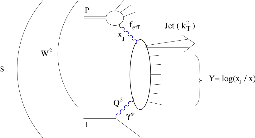
Figure 1: Production of a forward jet in a proton-lepton collision. The kinematic variables of the problem are displayed. $Q^{2}$ is the virtuality of the photon that undergoes the hadronic interaction. $s$ and $W^{2}$ are the total energies squared in the lepton-proton and photon-proton collisions respectively. $k_{T}$ is the transverse momentum of the forward jet and $x_{J}$ is its longitudinal momentum fraction with respect to the incident proton. $Y$ is the rapidity interval between the two hard probes.

$$\frac{d\sigma_{q\bar{q}}}{dx_{J}dk_{T}^{2}}(r)=\frac{\pi N_{c}}{16k_{T}^{2}}f_{eff}(x_{J},k_{T}^{2})\int_{0}^{\infty}d\bar{r}\ J_{0}(k_{T}\bar{r})\ \frac{\partial}{\partial\bar{r}}{\left({\bar{r}\frac{\partial}{\partial\bar{r}}\ \sigma_{(q\bar{q})(gg)}(r,\bar{r},Y)}\right)}$$ (5)

with $Y\!=\!\log(x_{J}\!/\!x)$ the rapidity assumed to be very large. $\sigma_{(q\bar{q})(gg)}(r,\bar{r},Y)$ is the cross-section in the collision of a $q\bar{q}$ dipole of size $r$ with a $gg$ dipole of size $\bar{r}$ with total rapidity $Y.$ $f_{eff}(x_{J},k_{T}^{2})$ is the effective parton distribution function and resums the leading logarithms $\log(k_{T}^{2}/\Lambda_{QCD}^{2}).$ It has the following expression

$$f_{eff}(x_{J},k_{T}^{2})=g(x_{J},k_{T}^{2})+\frac{C_{F}}{N_{c}}{\left({q(x_{J},k_{T}^{2})+\bar{q}(x_{J},k_{T}^{2})}\right)}\ ,$$ (6)

where $g$ (resp. $q$, $\bar{q}$) is the gluon (resp. quark, antiquark) distribution function in the incident proton.

Let us comment formula (5). Since the forward jet measurement involves perturbative values of $k_{T}$ and moderate values of $x_{J},$ it is not surprising that formula (5) features the collinear factorization of $f_{eff};$ note also that $k_{T}^{2}$ has been chosen as the factorization scale. The remaining hard interaction is between a $gg$ dipole and the incident $q\bar{q}$ dipole of size $r.$ The $gg$ dipole emerges as the effective degree of freedom for the gluon emission at high energies marq . This feature has been pointed out several times ggdip .

Formulae (1)-(6) express the forward-jet observable (1) in terms of the cross-section $\sigma_{(q\bar{q})(gg)}$ which contains the high-energy QCD dynamics: the problem is analogous to the one of onium-onium scattering. In the next subsection (II-B), we deal with the BFKL energy regime for which the interaction between the $q\bar{q}$ dipole and $gg$ dipole is restricted to a Pomeron exchange. In that case of course, our formulation is equivalent to the $k_{T}-$factorization approach. In subsection (II-C), we go beyond $k_{T}-$factorization and investigate the saturation regime in which $\sigma_{(q\bar{q})(gg)}$ a priori contains any number of gluon exchanges.

II.2 The BFKL energy regime

The BFKL $q\bar{q}$-$gg$ dipole-dipole cross-section reads (see for instance samuel )

$$\sigma^{BFKL}_{(q\bar{q})(gg)}(r,\bar{r},Y)=2\pi\alpha_{s}^{2}r^{2}{\int\frac{d\gamma}{2i\pi}}\frac{{\left({\bar{r}/r}\right)}^{2\gamma}}{\gamma^{2}(1\!-\!\gamma)^{2}}\ \exp{{\left({\displaystyle\frac{\alpha_{s}N_{c}}{\pi}\chi(\gamma)Y}\right)}}$$ (7)

with the complex integral running along the imaginary axis from $1/2\!-\!i\infty$ to $1/2\!+\!i\infty$ and with the BFKL kernel given by

$$\chi(\gamma)=2\psi(1)-\psi(1-\gamma)-\psi(\gamma)$$ (8)

where $\psi(\gamma)$ is the logarithmic derivative of the Gamma function. It comes about when the interaction between the $q\bar{q}-$dipole and the $gg-$dipole is restricted to a two-gluon exchange. Summing the leading-logarithmic contributions of ladders with any number of real gluon emissions, one obtains the BFKL Pomeron and the resulting growth of the cross-section with rapidity.

Inserting (7) in (5) and (2), one obtains

$$\frac{d\sigma^{\gamma*p\!\rightarrow\!JX}_{T,L}}{dx_{J}dk_{T}^{2}}=\frac{\pi^{2}N_{c}\alpha_{s}^{2}}{4k_{T}^{2}Q^{2}}f_{eff}(x_{J},k_{T}^{2}){\int\frac{d\gamma}{2i\pi}}{\left({\frac{Q^{2}}{k_{T}^{2}}}\right)}^{\gamma}\frac{4^{\gamma}\Gamma(\gamma)\ \phi^{\gamma}_{T,L}(\gamma)}{(1\!-\!\gamma)\ \Gamma(2\!-\!\gamma)}\exp{{\left({\displaystyle\frac{\alpha_{s}N_{c}}{\pi}\chi(\gamma)Y}\right)}}$$ (9)

where we have defined the following Mellin-transforms

$$\phi^{\gamma}_{T,L}(\gamma)=\int d^{2}r(r^{2}Q^{2})^{1-\gamma}\int_{0}^{1}dz|\psi_{T,L}^{\gamma}(r,z;Q)|^{2}$$ (10)

which are given by

$${\left({\begin{array}[]{cc}\phi^{\gamma}_{T}(\gamma)\\ \phi^{\gamma}_{L}(\gamma)\end{array}}\right)}=\frac{2\alpha_{em}N_{c}}{\pi}\sum_{q}e_{q}^{2}\frac{1}{4^{\gamma}\gamma}\frac{\Gamma^{2}(1+\gamma)\Gamma^{2}(1-\gamma)\Gamma^{2}(2-\gamma)}{\Gamma(2-2\gamma)\Gamma(2+2\gamma)(3-2\gamma)}{\left({\begin{array}[]{cc}(1+\gamma)(2-\gamma)\\ 2\gamma(1-\gamma)\end{array}}\right)}\ .$$ (11)

Inserting formula (9) into (1) gives the forward-jet cross-section in the BFKL energy regime. One can easily show that the result is identical to the one obtained using $k_{T}-$factorization fjets ; ktfac . The only undetermined parameter is $\bar{\alpha}\!\equiv\!\alpha_{s}N_{c}/\pi$ (with $\alpha_{s}$ the strong coupling constant kept fixed) which appears in the exponential in formula (9).

II.3 The saturation regime

Contrary to the BFKL case, the onium-onium cross-section in the saturation regime has not yet been computed from QCD. Studies are being carried out to identify the dominant terms in the multiple gluon exchanges edal ; poml1 ; poml2 ; poml3 but the cross-section $\sigma^{sat}_{(q\bar{q})(gg)}$ remains unknown. To take into account saturation effects, we are led to use a phenomenological parametrization. We consider the following model introduced in mpr which is inspired by the GBW approach:

$$\sigma^{sat}_{(q\bar{q})(gg)}(r,\bar{r},Y)=4\pi\alpha_{s}^{2}\sigma_{0}{\left({1-\exp{\left({-\frac{r_{\rm eff}^{2}(r,\bar{r})}{4R_{0}^{2}(Y)}}\right)}}\right)}\ .$$ (12)

The dipole-dipole effective radius $r^{2}_{\rm eff}(r,\bar{r})$ is defined through the two-gluon exchange:

$$4\pi\alpha_{s}^{2}r^{2}_{\rm eff}(r,\bar{r})\equiv\sigma^{BFKL}_{(q\bar{q})(gg)}(r,\bar{r},0)=4\pi\alpha_{s}^{2}\min(r^{2}\!,\bar{r}^{2})\left\{1\!+\!\log\frac{\max(r\!,\bar{r})}{\min(r\!,\bar{r})}\right\}\ .$$ (13)

For the saturation radius we use the parametrization $R_{0}(Y)\!=\!e^{-\frac{\lambda}{2}\left(Y-Y_{0}\right)}/Q_{0}$ with $Q_{0}\!\equiv\!1\ GeV.$

Let us express the cross-section in terms of a double Mellin-transform:

$$\sigma^{sat}_{(q\bar{q})(gg)}(r,\bar{r},Y)=4\pi\alpha_{s}^{2}\sigma_{0}{\int\frac{d\gamma}{2i\pi}}{\int\frac{d\tau}{2i\pi}}{\left({\frac{r^{2}}{4R_{0}^{2}(Y)}}\right)}^{1-\gamma}{\left({\frac{\bar{r}^{2}}{4R_{0}^{2}(Y)}}\right)}^{\tau}g(\gamma,\tau)$$ (14)

with

$$g(\gamma,\tau)=\int_{0}^{\infty}du^{2}\int_{0}^{\infty}d\bar{u}^{2}u^{2\gamma-4}\bar{u}^{-2\tau-2}{\left({1-e^{-r_{eff}^{2}(u,\bar{u})}}\right)}=\frac{2\Gamma{(\gamma-\tau)}}{1+\tau-\gamma}\ \left\{\Psi(1,3\!+\!\tau\!-\!\gamma,2\tau)+\Psi(1,3\!+\!\tau\!-\!\gamma,2\!-\!2\gamma)\right\}$$

$$0<Re(\tau),\;Re(\gamma),\;Re(\gamma-\tau)<1\hskip 341.43306pt$$ (15)

where the confluent hypergeometric function of Tricomi $\Psi(1,a,b)$ can be expressed prud in terms of incomplete Gamma functions. Inserting (14) in (5) and (2), one obtains

$$\frac{d\sigma^{\gamma*p\!\rightarrow\!JX}_{T,L}}{dx_{J}dk_{T}^{2}}=\frac{\pi^{2}N_{c}\alpha_{s}^{2}\sigma_{0}}{8Q^{2}k_{T}^{2}R_{0}^{2}(Y)}f_{eff}(x_{J},k_{T}^{2}){\int\frac{d\gamma}{2i\pi}}(4Q^{2}R_{0}^{2}(Y))^{\gamma}\phi^{\gamma}_{T,L}(\gamma){\int\frac{d\tau}{2i\pi}}(4k_{T}^{2}R_{0}^{2}(Y))^{-\tau}\frac{4^{\tau}\tau^{2}\Gamma(\tau)}{\Gamma(1\!-\!\tau)}\ g(\gamma,\tau)\ .$$ (16)

Inserting formula (16) into (1) gives our parametrization of the forward-jet cross-section in the saturation regime. The parameters are $\lambda,$ $Y_{0}$ and the normalization $\sigma_{0}.$

II.4 Fixing the parameters

The first sets of data published by the H1 h199 and ZEUS zeus99 collaborations regarded the measurement of $d\sigma/dx.$ In previous studies, we fitted the BFKL-LL fjets and saturation parametrization mnj on those data with the cut $x\!<\!10^{-2}.$ Despite corresponding different energy regimes, in both cases we obtained good descriptions with $\chi^{2}$ values of about 1. The obtained values of the parameters and the $\chi^{2}$ of the fits are given in Table I.

fit	parameters	$1/R_{0}(Y\!=\!0)$	$\chi^{2}(/\mbox{d.o.f.})$
BFKL-LL	$4\bar{\alpha}\log(2)\!=\!0.430$	——	12 (/13)
strong sat.	$\lambda=0.402$ and $Y_{0}=-0.82$	1.18 Gev	6.8 (/11)
weak sat.	$\lambda=0.370$ and $Y_{0}=8.23$	0.22 Gev	8.3 (/11)

Table 1: Results of the BFKL and saturation fits to the first HERA forward-jet data. The saturation fits shows two independent solutions showing either strong or weak saturation parameters (see text).

In the BFKL-LL case, the only parameter is $\bar{\alpha}$ and the value obtained was $4\bar{\alpha}\log(2)\!=\!0.430.$ For the saturation fit, the two relevant parameters are $\lambda$ and $Y_{0}$ and the fit showed two $\chi^{2}$ minima for $(\lambda\!=\!0.402,Y_{0}\!=\!-0.82)$ and $(\lambda\!=\!0.370,Y_{0}\!=\!8.23).$ We shall refer to the first (resp. second) solution as a strong (resp. weak) saturation parametrization. Indeed, the first saturation minimum corresponds to strong saturation effects as, for typical values of $Y,$ the saturation scale $1/R_{0}$ is about 5 Gev which is the value of a typical $k_{T}.$ The second saturation minima corresponds to small saturation effects and rather describes BFKL physics.

Along with formulae (9) and (16), the values of the parameters given in Table I completely determine the BFKL-LL predictions and two parametrizations for the saturation model. We are now going to compare these with the very recent data without any adjustment of the parameters. This will provide a strong test of those small$-x$ effects.

II.5 Comparison to the 2005 HERA data

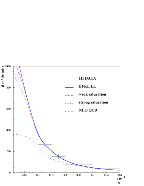
Figure 2: The forward-jet cross-section $d\sigma/dx.$ The points are measurement by the H1 (left plot) and ZEUS (right plot) collaborations. The lines are comparisons with BFKL-LL predictions (full lines) and the two saturation parametrizations (dotted and dashed lines). In both cases, there is good agreement with the data. For comparison, fixed-order QCD predictions at NLO are also displayed.

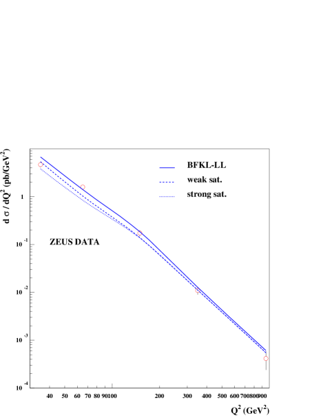
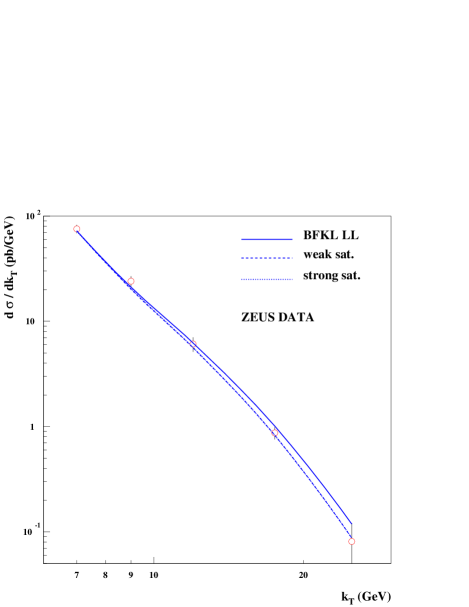
Figure 3: The forward-jet cross-sections $d\sigma/dQ^{2}$ (left plot) and $d\sigma/dk_{T}$ (right plot). The points are measurement by the ZEUS collaboration. The lines are comparisons with BFKL-LL predictions (full lines) and the two saturation parametrizations (dotted and dashed lines). For the two observables, there is good agreement with the data.

We want to compare the cross-section (1) obtained from the BFKL-LL prediction (9) and the saturation parametrization (16) with the new data coming from measurements performed at HERA zeusnew ; h1new . On one side, our theoretical results are for the cross-section (1) which is differential with respect to all four kinematic variables $x,$ $Q^{2},$ $x_{J},$ and $k_{T}.$ On the other side, HERA data concern observables which are less differential: $d\sigma/dx,$ $d\sigma/dQ^{2},$ $d\sigma/dk_{T}^{2},$ and $d\sigma/dxdQ^{2}dk_{T}^{2}.$ Therefore, on the top of the Mellin integrations in (9) and (16), one has to carry out a number of integrations over the kinematic variables which have to be done taking into account the kinematic cuts applied by the different experiments. A detailed description of how we performed those integrations in given in Appendix A and the resulting cross-sections that can be compared to the data are given in Appendix B. The method allows for a direct comparison of the data with theoretical predictions but it does not allow to control the overall normalization. In the following studies, we therefore compare only spectra and will not refer to normalizations anymore. As already mentioned, one does not adjust any of the parameters of Table I.

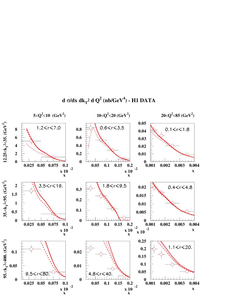
Figure 4: The forward-jet cross-section $d\sigma/dxdQ^{2}dk_{T}^{2}.$ The points are measurement by the H1 collaboration. The lines are comparisons with BFKL-LL predictions (full lines) and the two saturation parametrizations (dotted and dashed lines for strong and weak saturation respectively). In the regime where on expects small$-x$ effects to be important ($r\!\equiv\!k_{T}^{2}/Q^{2}\!\sim\!1$), there is a good description of the data. In the regime where $r\!\gg\!1,$ the small$-x$ parametrizations do not reproduce the data as expected from the hierarchy of the hard scales.

Let us start with the observable $d\sigma/dx$ which has been measured by both the H1 and ZEUS collaborations and which now features lower values of $x$ than the first measurements. The comparison is displayed in Fig.2, the three small$-x$ parametrizations describe very well the data. One cannot really distinguish between the three curves, except at small values of $x$ where one starts to see a difference: the BFKL curve is above the weak-saturation curve which is itself above the strong-saturation curve. However the main conclusion is that the data seem to feature the BFKL growth, when going to small values of $x.$ For comparison, the fixed-order QCD predictions at NLO computed in zeusnew ; h1new with the DISENT Monte-Carlo program disent are reproduced in Fig.2. At the lowest values of $x,$ they do not reproduce the data as they are about a factor 1.5 to 2.5 below depending on the experiment and the error bars. Even adding a resolved-photon component to the NLO predictions h1new does not pull them within the uncertainties, contrary to what happened for the previous data respho . This is an interesting difference with the forward-pion case basu for which it seems that no higher-order effect other than a NLO resolved-photon contribution is needed.

In Fig.3 are represented the two other single differential cross-sections that we shall briefly discuss: $d\sigma/dQ^{2}$ and $d\sigma/dk_{T}$ measured by the ZEUS collaboration. One can see again that the three small$-x$ parametrizations agree well with the data, it is a strong result that one is able to describe the $Q^{2}$ and $k_{T}$ spectra without any adjustment of the parameters as they were only fitted to describe the $x$ dependence.

We shall finally compare our predictions with the triple differential cross-section $d\sigma/dxdQ^{2}dk_{T}^{2}$ measured by the H1 collaboration. The interesting part of this measurement is that it has been carried out in 9 different bins of $r\!\equiv\!k_{T}^{2}/Q^{2}$ from $0.1\!<\!r\!<\!1.8$ to $9.5\!<\!r\!<\!80.$ This allows to test the limits of our parametrizations which are supposed to be valid only when $r\!\sim\!1$ as they do not take into account any transverse momentum ordering of the gluons emitted in rapidity between the forward jet and the photon. The comparisons with the data are shown on Fig.4 and one sees the expected trend. The bins which have $r\!\sim\!1$ are well described by the small$-x$ parametrizations while the others are not: for the latter, we overshoot the data as the BFKL rise towards small values of $x$ is too steep. Interestingly enough, the trend is reversed for QCD predictions at NLO: they describe better the data which feature large values of $r.$ These observations favor the need of the BFKL resummation to describe the $r\!\sim\!1$ data. The large$-r$ bins also exhibit a limitation of the saturation model as one can see that the strong saturation parametrization lies above the weak saturation parametrization. Such a behavior indicates that the model should not be used when $k_{T}^{2}\!\gg\!Q^{2}.$

Let us comment further on the two saturation parametrizations. While the BFKL formula (9) is a QCD prediction as it is computed from Feynman diagrams bfkl , the saturation parametrization (16) is a phenomenological model. The fact that it describes well the data does not call for the same conclusions as in the BFKL case. It only exhibits that, as it is the case for a number of observables, data are compatible with saturation effects even at energies which do not require them. In other words, the forward-jet measurement at the present energies cannot distinguish between saturation and BFKL effects; one would start seeing a significant difference at higher energies.

It is the purpose of the next section to look for such differences, by studying another process similar to forward-jets, namely Mueller-Navelet jets, at LHC energies.

III Towards the LHC: Mueller-Navelet jets

Mueller-Navelet jet production in a proton-proton collision is represented in Fig.5 with the different kinematic variables. We denote $\sqrt{S}$ the total energy of the collision, $k_{1}$ and $k_{2}$ the transverse momenta of the two forward jets and $x_{1}$ and $x_{2}$ their longitudinal fraction of momentum with respect to the protons as indicated on the figure. In the following, we compute the Mueller-Navelet jet cross-section in the high-energy limit, recall the BFKL predictions and formulate our saturation model. We then display predictions for observables which can be measured at the LHC.

III.1 Formulation

As in the original paper mnj , we consider the cross-section differential with respect to $x_{1}$ and $x_{2}$ and integrated over the transverse momenta of the jets with $k_{1}\!>\!Q_{1}$ and $k_{2}\!>\!Q_{2}.$ $Q_{1}$ and $Q_{2}$ represent then experimental $k_{T}-$cuts. Considering the high energy limit, the QCD cross-section for Mueller-Navelet jet production reads marq ; marpes :

$$\frac{d\sigma^{pp\!\rightarrow\!JXJ}}{dx_{1}dx_{2}}=\frac{\pi^{2}N_{c}^{2}}{64}f_{eff}(x_{1},Q_{1}^{2})f_{eff}(x_{2},Q_{2}^{2})\int_{0}^{\infty}dr\int_{0}^{\infty}d\bar{r}\ Q_{1}J_{1}(Q_{1}r)Q_{2}J_{1}(Q_{2}\bar{r})\ \sigma_{(gg)(gg)}(r,\bar{r},Y)$$ (17)

with $Y\!=\!\log(x_{1}x_{2}S/Q_{1}Q_{2})$ the rapidity assumed to be very large. $\sigma_{(gg)(gg)}(r,\bar{r},Y)$ is the cross-section in the collision of two $gg$ dipoles of size $r$ and $\bar{r}$ with rapidity total Y. As before $f_{eff}$ is the effective parton distribution function (6).

Let us comment formula (17). As before, each forward jet involves perturbative values of transverse momenta and moderate values for $x_{1}$ and $x_{2}.$ This explains the collinear factorization of the two functions $f_{eff};$ here we have taken the factorization scales to be $Q^{2}_{1}$ and $Q^{2}_{2}.$ The remaining hard interaction is between two $gg$ dipoles: as we have seen in the previous section, each of them describes a gluon emission at high energies. Formula (17) expresses the Mueller-Navelet jet observable in terms of the cross-section $\sigma_{(gg)(gg)}$ which contains the high-energy QCD dynamics. This is the similarity with the forward-jet case: the problem is also analogous to the one of onium-onium scattering.

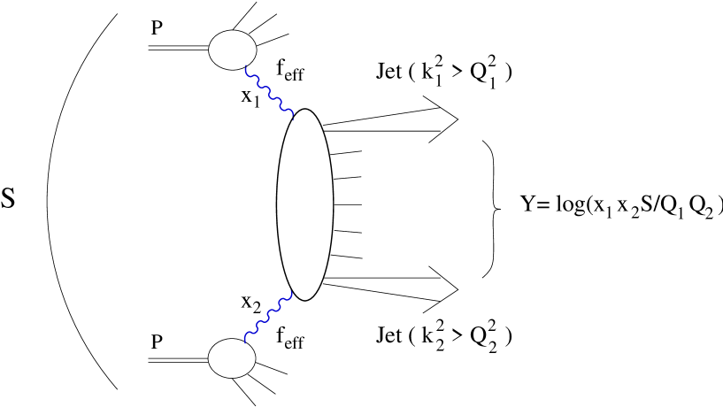
Figure 5: Mueller-Navelet jet production in a proton-proton collision. The kinematic variables of the problem are displayed. $S$ is the total energy squared, $k_{1}$ and $k_{2}$ are the transverse momenta of the jets and $x_{1}$ and $x_{2}$ are their longitudinal momentum fraction with respect to the incident protons. $Y$ is the rapidity interval between the hard probes.

Let us first consider the BFKL energy regime, the $gg$-$gg$ dipole-dipole cross-section reads

$$\sigma^{BFKL}_{(gg)(gg)}(r,\bar{r},Y)=\frac{2\pi N_{c}\alpha_{s}^{2}}{C_{F}}\ r^{2}{\int\frac{d\gamma}{2i\pi}}\frac{{\left({\bar{r}/r}\right)}^{2\gamma}}{\gamma^{2}(1\!-\!\gamma)^{2}}\ \exp{{\left({\displaystyle\frac{\alpha_{s}N_{c}}{\pi}\chi(\gamma)Y}\right)}}$$ (18)

which combined with (17) gives

$$\frac{d\sigma^{BFKL}}{dx_{1}dx_{2}}=\frac{\pi^{3}N_{c}^{3}\alpha_{s}^{2}}{8C_{F}Q_{1}^{2}}f_{eff}(x_{1},Q_{1}^{2})f_{eff}(x_{2},Q_{2}^{2}){\int\frac{d\gamma}{2i\pi}}\frac{{\left({Q_{1}/Q_{2}}\right)}^{2\gamma}}{\gamma(1\!-\!\gamma)}\ \exp{{\left({\displaystyle\frac{\alpha_{s}N_{c}}{\pi}\chi(\gamma)Y}\right)}}\ .$$ (19)

One can easily show that the result is identical to the one obtains using $k_{T}-$factorization mnj . As in the forward-jet case, the only undetermined parameter is $\bar{\alpha}$ which appears in the exponential in formula (19). We shall consider in this study the same value that was used for forward jets, that is $\bar{\alpha}\!=\!0.16.$

For the saturation parametrization, we use the following $gg$-$gg$ dipole-dipole cross-section:

$$\sigma^{sat}_{(gg)(gg)}(r,\bar{r},Y)=\frac{4\pi N_{c}\alpha_{s}^{2}}{C_{F}}\ \sigma_{0}{\left({1-\exp{\left({-\frac{r_{\rm eff}^{2}(r,\bar{r})}{4R_{0}^{2}(Y)}}\right)}}\right)}\ .$$ (20)

which up to the normalization is the same as (12). The effective radius $r_{eff}$ is defined by formula (13) and the saturation radius by $R_{0}(Y)\!=\!e^{-\frac{\lambda}{2}\left(Y-Y_{0}\right)}/Q_{0}$ with $Q_{0}\!\equiv\!1\ GeV.$ Inserting (20) into (17), one obtains marpes

$$\frac{d\sigma^{sat}}{dx_{1}dx_{2}}=\frac{\pi^{3}N_{c}^{3}\alpha_{s}^{2}\sigma_{0}}{16C_{F}}f_{eff}(x_{1},Q_{1}^{2})f_{eff}(x_{2},Q_{2}^{2})\left\{1-2R_{0}^{2}(Y)Q_{1}Q_{2}\int_{1}^{\infty}\frac{du}{1+\log(u)}\ I_{1}{\left({\frac{2Q_{1}Q_{2}uR_{0}^{2}(Y)}{1+\log(u)}}\right)}\right.$$

$$\left.\times\left[\exp{\left({-\displaystyle\frac{Q_{1}^{2}+u^{2}Q_{2}^{2}}{1+\log(u)}R_{0}^{2}(Y)}\right)}+\exp{\left({-\displaystyle\frac{Q_{2}^{2}+u^{2}Q_{1}^{2}}{1+\log(u)}R_{0}^{2}(Y)}\right)}\right]\right\}\ .$$ (21)

In the following we consider only the strong saturation parametrization to display what could be the maximal expected effects at the LHC. The parameters are $\lambda\!=\!0.402$ and $Y_{0}\!=\!-0.82.$ The normalization $\sigma_{0}$ is a priori not determined but we have fixed it so that at large momenta and small $Y,$ one obtains the BFKL result.

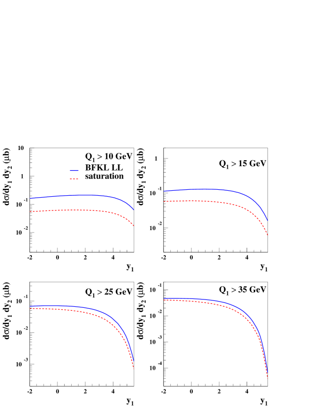
Figure 6: The Mueller-Navelet jet cross-section $d\sigma/dy_{1}dy_{2}$ as a function of $y_{1}$ for different values of $Q_{1}.$ The kinematics of the other jet are fixed at $Q_{2}\!=\!30\ \mbox{GeV}$ and $y_{2}\!=\!-4.5.$ The full lines are BFKL-LL predictions and the dashed lines are the saturation parametrization.

III.2 Phenomenology

Figure 7: Ratio of the saturation and BFKL-LL Mueller-Navelet jet cross-sections $d\sigma/dy_{1}dy_{2}$ as a function of $y_{1}$ for different values of $Q_{1}.$ The kinematics of the other jet are fixed at $Q_{2}\!=\!70\ \mbox{GeV}$ and $y_{2}\!=\!-3.5.$

We are going to study the dependence of the cross-sections (19) and (21) as a function of the different kinematic variables $x_{1},$ $x_{2},$ $Q_{1},$ and $Q_{2}.$ We want to consider large rapidities $Y$ which implies very forward jets and therefore large values of $x_{1}$ and $x_{2}.$ The well-known problem is that the cross-section is then damped by the parton distribution functions which at large $x$ become very small. This prevents one to see the BFKL enhancement of the hard part of the cross-section with rapidity.

A way out of this problem is to consider the following observables ${\cal R}_{S/\tilde{S}}:$

$${\cal R}_{S/\tilde{S}}\equiv\frac{d\sigma^{pp\!\rightarrow\!JXJ}}{dx_{1}dx_{2}}(Q_{1},Q_{2},S)\Big{/}\frac{d\sigma^{pp\!\rightarrow\!JXJ}}{dx_{1}dx_{2}}(Q_{1},Q_{2},\tilde{S})\ ,$$ (22)

in other words, cross-section ratios for same jet kinematics and two different values of the total energy squared ($S$ and $\tilde{S}$). The advantage of such observables is that they are independent of the parton densities and allow to study more quantitatively the influence of small$-x$ effects fjets ; marpes ; mpr . For instance the BFKL-LL prediction is (via a saddle point approximation):

$${\cal R}_{S/\tilde{S}}\simeq{\left({\frac{S}{\tilde{S}}}\right)}^{4\bar{\alpha}\log(2)}.$$ (23)

The experimental verification of this at the Tevatron mnjtev was not conclusive. The data were found above the prediction (23), however it has been argued schmidt that the measurement was biased by the use of upper $k_{T}-$cuts, the choice of equal lower $k_{T}-$cuts, and hadronization corrections. The ratios (22) also display in a clear way the saturation effects marpes ; mpr which lead to ratios that, as a function of $Q_{1}$ and $Q_{2},$ go from the value (23) to 1 as the momentum cuts decrease into the saturation region (see Fig.4 in Ref. mpr and Fig.3,4 in Ref. marpes ).

There is however an important experimental limitation to carry out the measurement (22): it would require to run the LHC at two different center-of-mass energies. If it turns out not to be possible, then one should settle for the cross-section $d\sigma/dx_{1}dx_{2}.$ We shall now exhibit some of its characteristics, fixing the LHC center-of-mass energy at $\sqrt{S}\!=\!14\ \mbox{TeV}.$ Also the absolute normalization is fixed to reproduce the Tevatron data at $\sqrt{S}\!=\!1.8\ \mbox{TeV}$ published in mnjtev . These data feature somewhat large error bars which leads to a significant uncertainty on the normalization for the LHC predictions.

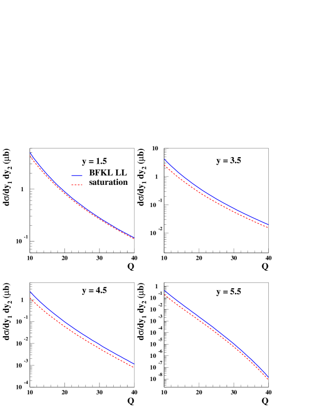
Figure 8: The Mueller-Navelet jet cross-section $d\sigma/dy_{1}dy_{2}$ as a function of $Q\!\equiv\!Q_{1}\!=\!Q_{2}$ for different values of $y\!\equiv\!y_{1}\!=\!-y_{2}.$ The full lines are BFKL-LL predictions and the dashed lines are the saturation parametrization.

Let us introduce the rapidities of the two jets:

$$y_{1}=\log{\left({\frac{x_{1}\sqrt{S}}{Q_{1}}}\right)}\ ,\hskip 28.45274pty_{2}=-\log{\left({\frac{x_{2}\sqrt{S}}{Q_{2}}}\right)}\ .$$ (24)

We first considered the case where one of the two jets has fixed kinematics $Q_{2}\!=\!30\ \mbox{GeV}$ and $y_{2}\!=\!-4.5.$ We looked at the dependence of the cross-section $d\sigma/dy_{1}dy_{2}\!=\!x_{1}x_{2}\ d\sigma/dx_{1}dx_{2}$ as a function of the other jet kinematic variables. In Fig.6, we plotted the results for the BFKL-LL prediction (19) and the saturation parametrization (21) where the different plots feature the $y_{1}$ dependence for different values of $Q_{1}.$ As expected, the cross-sections decrease quickly as $y_{1}$ gets large which corresponds to $x_{1}$ getting closer to one. For each value of $Q_{1},$ one cannot really see a difference between the behaviors of the BFKL and saturation curves as a function of $y_{1}.$ However the relative normalization between the two curves is quite sensitive to the value of $Q_{1}.$ This is better exhibited on Fig.7 where one displays the ratio of the saturation and BFKL results of Fig.6. The ratio goes down to about 0.3 for $Q_{1}\!=\!10\ \mbox{GeV}$ which represents a significant difference between the BFKL and saturation predictions. Note that this difference does not appear to be that large on Fig.6 where the cross-sections are plotted.

The second case we considered is the symmetric case $Q\!\equiv\!Q_{1}\!=\!Q_{2}$ and $y\!\equiv\!y_{1}\!=\!-y_{2}$ which allows to go to bigger values of $Y.$ We looked at the dependence of the cross-section $d\sigma/dy_{1}dy_{2}$ as a function of $Q$ and $y.$ In Fig.8, we plotted the results for the BFKL prediction (19) and the saturation parametrization (21) where the different plots feature the $Q$ dependence for different values of $y.$ In this case, the cross-section falls even faster when $y$ gets big as both $x_{1}$ and $x_{2}$ get close to 1. Again, because of that, one does not see on the plot the difference between the BFKL and the saturation curves, yet it is still quite big as shown on Fig.9 where we have displayed the ratio of the saturation and BFKL results of Fig.8. For $y\!=\!5.5$ and $Q$ decreasing down to $10\ \mbox{GeV},$ the ratio goes down to about 0.4.

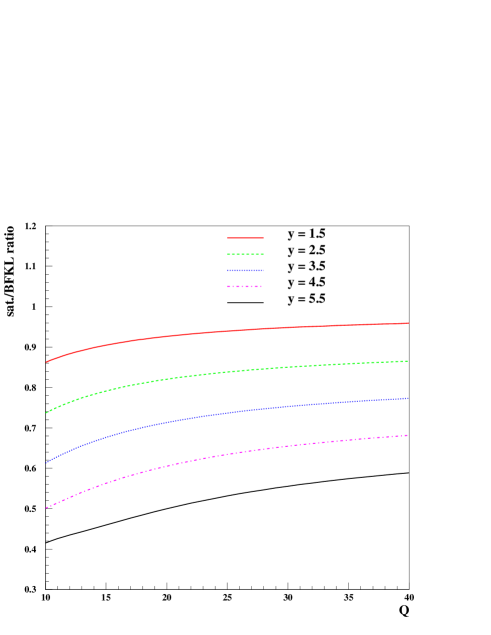
Figure 9: Ratio of the saturation and BFKL-LL Mueller-Navelet jet cross-sections $d\sigma/dy_{1}dy_{2}$ as a function of $Q\!\equiv\!Q_{1}\!=\!Q_{2}$ for different values of $y\!\equiv\!y_{1}\!=\!-y_{2}.$

We did not include in this study the weak saturation parametrization, the corresponding curves would lie in between the BFKL and strong saturation curves which are displayed, and even is closer to the BFKL curve. There is a number of other plots one could study showing other dependences of $d\sigma/dy_{1}dy_{2}$ but they are not needed for drawing our conclusions: testing BFKL effects and saturation effects with the observable $d\sigma/dy_{1}dy_{2}$ at the LHC will be a major experimental challenge as one will have to measure cross-sections with a great precision. We insist that this is due to the fact that the parton distribution functions at large $x$ really damp the cross-section. Obtaining a high accuracy is not unfeasible because of the high luminosity at the LHC but this will require a very good understanding of the systematics errors. However we would like to emphasize the fact that better tests of small$-x$ effects could be realized with the measurement of the ratio ${\cal R}_{S/\tilde{S}},$ see formula (22).

IV Conclusions

Let us summarize the main results of the paper. The first part of the work was devoted to the study of the forward-jet measurement. We started by computing the QCD cross-section for forward-jet production (1) in the high-energy (small$-x$) limit. We recalled the BFKL-LL predictions (9) and also formulated the phenomenological model (16) that takes into account saturation effects. We then compared the BFKL and saturation-model predictions to the recent data from HERA for a number of observables: $d\sigma/dx,$ $d\sigma/dQ^{2},$ $d\sigma/dk_{T}^{2},$ and $d\sigma/dxdQ^{2}dk_{T}^{2}.$

We obtained a very good agreement with the BFKL predictions and saturation parametrizations also show compatibility with the data. Along with the fact that QCD at NLO predictions do not reproduce the small$-x$ data, this observation leads us to the conclusion that the present forward-jet data display the BFKL enhancement when going to small values of $x.$

However, to make a definitive statement, one would have to make comparisons with BFKL predictions at next-to-leading-logarithmic (NLL) accuracy. The latter are under investigations and will hopefully be available soon. In the mean time, let us discuss the expected qualitative impact of these BFKL-NLL corrections. Because we are describing a kinematic regime in which $k_{T}^{2}\!\sim\!Q^{2},$ one can infer that they should be small. For instance, the contribution coming from the running of the coupling between those two scales would be unimportant. By comparison, the BKFL-NNL corrections seem to be very large for the proton structure function measurement nll , in which case one easily understands why: the evolution takes place in a large range, from the soft proton scale up to the hard scale $Q^{2}.$ The situation is much different for forward jets.

In the second part of the paper, we investigated small$-x$ effects for Mueller-Navelet jets in the LHC energy range, using the parameters that successfully describe forward-jets at HERA. We compared the BFKL-LL predictions (19) with those of the saturation model (21) and concluded that the measurement of the simple cross-section will require a great precision to test the different scenarios. We argued that a better option to look for small$-x$ effects was to measure the ratio of cross-sections (22) which implies running the LHC at two different energies.

On longer time scales, the international linear collider would give the opportunity to measure the virtual photon-virtual photon total cross-section at very high energies. This would also offer great possibilities gambfkl ; gamsat for testing the BFKL enhancement and the saturation regime of QCD.

Appendix A: on the integration method

To compare the forward-jet cross-section (1) obtained from the BFKL-LL prediction (9) and the saturation parametrization (16) with the data for observables which are less differential ($d\sigma/dx,$ $d\sigma/dQ^{2},$ $d\sigma/dk_{T}^{2},$ and $d\sigma/dxdQ^{2}dk_{T}^{2}$), one has to carry out a number of integrations over the kinematic variables. They have to be done while properly taking into account the kinematic cuts applied by the different experiments. This Appendix deals with these issues.

Let us start from the quadruple differential cross-section $d\sigma/dxdQ^{2}dx_{J}dk_{T}^{2},$ see formula (1). First one performs the Mellin integrations of (9) and (16). Then we choose the appropriate variables for the remaining integrations: to avoid numerical problems in the integral calculations, we chose variables which lead to the weakest possible dependence of the differential cross-section. We noticed that the best choice is $1/Q^{2},$ $1/k_{T}^{2},$ $\log(1/x_{J}),$ and $\log(1/x).$ Since the experimental measurements are not differential with respect to $x_{J},$ we carry out the integration

$$\frac{d^{(3)}\sigma}{dxdQ^{2}dk_{T}^{2}}=\int\frac{x_{J}\ d^{(4)}\sigma}{dxdQ^{2}dx_{J}dk_{T}^{2}}\ d\log{\left({\frac{1}{x_{J}}}\right)}\ .$$

With the BFKL-LL formula (9), the convergence is fast enough so that one can perform all the remaining integrations to obtain any of the four observables mentioned above. With the saturation formula (16), because of the extra Mellin integration and the time it takes to compute the functions $\Psi,$ performing all the remaining integrations would require important numerical work. We chose to use another method to obtain the cross-sections in that case. We shall describe it now with the example of $d\sigma/dx.$

For a given value of $x,$ the first step is to compute the differential cross-section

$$\frac{d\sigma^{BFKL}}{dx}=\int Q^{4}k_{T}^{4}\ \frac{d^{(3)}\sigma^{BFKL}}{dxdQ^{2}dk_{T}^{2}}\ d{\left({\frac{1}{Q^{2}}}\right)}\ d{\left({\frac{1}{k_{T}^{2}}}\right)}\$$

for the BFKL case. The second step is to compute the bin center ($k_{TC}^{2}$, $Q_{C}^{2}$) defined as follows:

$$\frac{d^{(3)}\sigma^{BFKL}}{dxdQ^{2}dk_{T}^{2}}(Q_{C}^{2},k_{TC}^{2})\equiv\frac{d\sigma^{BFKL}/dx}{\int dQ^{2}dk_{T}^{2}}\ .$$

The bin center is thus the point in the $(k_{T}^{2},Q^{2})$ phase space where the differential cross-section in $k_{T}^{2}$ and $Q^{2}$ is equal to the integral over the bin divided by the bin size (we will specify the integration limits later on). The third step is to obtain the cross section for the saturation case. We compute the cross-section at the bin center ($k_{TC}^{2}$, $Q_{C}^{2}$):

$$\frac{d\sigma^{sat}}{dx}=\frac{d^{(3)}\sigma^{sat}}{dxdQ^{2}dk_{T}^{2}}(Q_{C}^{2},k_{TC}^{2})\ \int dQ^{2}dk_{T}^{2}\ .$$

This procedure is valid if the bin center does not change much between the BFKL and saturated cross-sections. In other words, it means that the difference between the BFKL and saturated cross-sections is small. We saw in Section II-E that this is indeed the case. The method is easily adapted to the case of $d\sigma/dQ^{2}$ for which one finds a bin center $(x_{C},k_{TC}^{2})$ for each value of $Q^{2}$ and to the case of $d\sigma/dk_{T}^{2}$ with a bin center $(x_{C},Q_{C}^{2})$ for each value of $k_{T}.$

For the triple differential cross-section $d\sigma/dxdQ^{2}dk_{T}^{2}$ which is measured as a function of $x,$ integrating over $x_{J}$ is not enough since one does not know the $(Q^{2},k_{T}^{2})$ bin-center. Instead, for a given value of $x,$ one integrates also over $Q^{2}$ and $k_{T}^{2}$ and then divide the result by the $Q^{2}$ and $k_{T}^{2}$ bin sizes to obtain $d\sigma/dxdQ^{2}dk_{T}^{2}.$ This is done for the BFKL case and one uses again the method described above to compute the cross-section in the saturation case.

The other difficulty arises when setting the integration limits as one has to take into account the correlations between the kinematic variables (for instance $y\!=\!Q^{2}/sx\!<\!1$) and the cuts applied by the experiments (for instance cuts on the forward jet phase space). There are two ways to take these into account: either appropriately set the limits of integration while computing the integrals or evaluate later the phase space correction due to the experimental cuts. We are going to use both, since it is not possible to include all experimental cuts while computing the integrals.

Table II is a list of the different set of cuts used by the H1 and ZEUS experiments to carry out their measurements. For the ZEUS cuts, we only consider what they call the “forward-BFKL phase space” which corresponds the most to the Regge limit kinematics. Refering to this table, let us enumerate the integration limits which are used for the different integral calculations:

• $d\sigma/dx$ for H1: We integrate over $1/k_{T}^{2}$ with the limit on $k_{T}^{2}$ defined by $0.5\!<\!k_{T}^{2}/Q^{2}\!<\!5$ (this is an extra cut that H1 applies to this measurement only), over $1/Q^{2}$ with $Q^{2}\!<\!sx$, and over $\log(1/x_{J})$ with $0.035\!<\!x_{J}\!<1$

• $d\sigma/dx$ for ZEUS: We integrate over $1/k_{T}^{2}$ with the limit on $k_{T}^{2}$ defined by $0.5\!<\!k_{T}^{2}/Q^{2}\!<\!2,$ over $1/Q^{2}$ with $Q^{2}\!<\!sx$, and over $\log(1/x_{J})$ with $2\!<\!\log(1/x_{J})\!<3$

• $d\sigma/dQ^{2}$ for ZEUS: We integrate over $1/k_{T}^{2}$ with the limit on $k_{T}^{2}$ defined by $0.5\!<\!k_{T}^{2}/Q^{2}\!<\!2,$ over $\log(1/x)$ with $x\!\geq\!Q^{2}/s$, and over $\log(1/x_{J})$ between 2 and 3

• $d\sigma/dk_{T}^{2}$ for ZEUS: We integrate over $\log(1/x)$ with $x\!\geq\!Q^{2}/s,$ over $1/Q^{2}$ with the limits on $Q^{2}$ defined by $0.5\!<\!k_{T}^{2}/Q^{2}\!<\!2,$ and over $\log(1/x_{J})$ between 2 and 3

• $d\sigma/dxdQ^{2}dk_{T}^{2}$ for H1: The $1/k_{T}^{2}$ and $1/Q^{2}$ limits of the integrals are defined by the bin values measured by the H1 collaboration with also the kinematic constraint $0.1\!<\!y=Q^{2}/sx\!<\!0.7.$ The $\log(1/x_{J})$ limits are obtained taking into account the cuts on the forward-jet angle which leads to $1.7354\!<\!\log(1/x_{J})\!<\!2.7942.$

H1	ZEUS
$E_{e}\geq 10$ GeV	$E_{e}\geq 10$ GeV
$0.1\leq y\leq 0.7$	$0.04\leq y\leq 1.$
$10^{-4}\leq x\leq 4.10^{-3}$
$5<Q^{2}<85$ GeV2	$Q^{2}>25$ GeV2
$k_{T}>3.5$ GeV	$k_{T}>6$ GeV
$7\leq\theta_{J}\leq 20$ degrees	$2<\eta_{J}<3$
$x_{J}>0.035$
	$0.5<k_{T}^{2}/Q^{2}<2$

Table 2: ZEUS (“forward-BFKL phase space”) zeusnew and H1 h1new cuts to define the forward-jet phase space. $E_{e}$ is the energy of the outgoing electron and $\eta_{J}\!=\!\log(1/x_{J})\!=\!-\log\tan(\theta_{J}/2).$ The other kinematic variables have been defined in the text.

The effects of the cuts defined in Table II which are not used above need to be computed using a toy Monte Carlo. They are modeled by bin-per-bin correction factors that multiply the cross-sections obtained as described above. This is how one proceeds: we generate flat distributions in the variables $1/k_{T}^{2},$ $1/Q^{2},$ $\log(1/x_{J}),$ and $\log(1/x)$ using reference intervals which include the whole experimental phase-space (the azimuthal angle of the jet is not used in the generation since all the cross-section measurements are independent of that angle). In practice, we get the correction factors by counting the numbers of events which fullfil the experimental cuts for each $x-$bin when we compute $d\sigma/dx$, each $Q^{2}-$bin when we compute $d\sigma/dQ^{2}$ and so on. The correction factors are obtained by the ratio of the number of events which pass the experimental cuts and the kinematic constraints to the number of events which fullfil only the kinematic constraints, i.e. the so-called reference bin. Of course the experimental or kinematic cuts which have been applied already while computing the integrals are not applied in this study to avoid double counting effects.

This method allows for a direct comparison of the data with theoretical predictions but it does not allow to control the overall normalization. This would require a full Monte-Carlo. Note that we did not use one in order to avoid any strong model dependence of the correction factors as they are only due to kinematic-cut effects. The derivation of the correction factors is independent of the theoretical input. They are given in Appendix B and they can be used to test any model suitable for the forward-jet cross-section, providing the same integration method as described above is used.

Appendix B: tables with correction factors and resulting cross-sections

In this section, we list the corrections factors that we obtained for the observables $d\sigma/dx$ (H1 and ZEUS), $d\sigma/dQ^{2}$ (ZEUS), $d\sigma/dk_{T}^{2}$ (ZEUS), and $d\sigma/dxdQ^{2}dk_{T}^{2}$ (H1). We also give the resulting cross-sections for the different points that we used to draw the curves on Fig.2, Fig.3, and Fig.4.

x	factor	bfkl-ll	weak sat.	strong sat.
0.00015	0.24	1200.	1046.	897.
0.0005	0.81	805.	785.	722.
0.0010	0.86	371.	365.	360.
0.0015	0.80	205.	202.	203.
0.0020	0.66	117.	114.	116.
0.0025	0.54	72.0	70.4	71.7
0.0030	0.45	47.1	45.9	46.9
0.0035	0.38	32.3	31.4	32.1
0.0040	0.31	22.5	21.8	22.3

x	factor	bfkl-ll	weak sat.	strong sat.
0.00075	0.13	39.3	34.5	31.1
0.0017	0.43	62.5	58.1	56.0
0.004	0.48	25.4	24.7	24.6
0.01	0.34	3.33	3.38	3.34
0.025	0.13	0.106	0.109	0.106

Table 3: Correction factors due to experimental cuts and the resulting corrected cross-sections for $d\sigma/dx$ in nb for BFKL-LL, weak saturation and strong saturation (see Fig.2). Left Table: for H1 cuts, right Table: for ZEUS cuts.

$Q^{2}$ (GeV2)	factor	bfkl-ll	weak sat.	strong sat.
35.	0.60	6.75	5.36	3.81
65.	0.70	1.40	1.03	0.843
150.	0.88	0.184	0.139	0.137
350.	0.88	0.0127	0.0112	0.0112
950.	0.96	0.000611	0.000549	0.000549

$k_{T}$ (GeV)	factor	bfkl-ll	weak sat.	strong sat.
7.	0.32	71.9	72.4	71.6
9.	0.31	21.1	20.2	20.4
12.	0.28	6.23	5.59	5.63
17.5	0.22	1.01	0.828	0.828
25.	0.15	0.119	0.0875	0.0875

Table 4: Correction factors due to experimental cuts and the resulting corrected cross-sections for BFKL-LL, weak saturation and strong saturation. Left Table: for $d\sigma/dQ^{2}$ in pb/GeV², right Table: for $d\sigma/dk_{T}$ in pb/GeV (see Fig.3).

$k_{T}^{2}$ (GeV2)	$Q^{2}$ (GeV2)	x	factor	bfkl-ll	weak sat.	strong sat.
$12.25<k_{T}^{2}<35$	$5<Q^{2}<10$	0.0002	0.065	8.28	7.85	4.40
		0.0004	0.065	3.86	3.69	2.53
		0.0006	0.065	2.04	1.96	1.51
		0.0008	0.065	0.705	0.674	0.591
		0.001	0.065	0.160	0.151	0.151
$12.25<k_{T}^{2}<35$	$10<Q^{2}<20$	0.0002	0.042	0.571	0.551	0.332
		0.0004	0.065	1.15	1.12	0.826
		0.0006	0.065	0.752	0.735	0.612
		0.0008	0.065	0.544	0.530	0.473
		0.001	0.065	0.416	0.406	0.376
		0.0012	0.065	0.289	0.280	0.275
		0.0014	0.065	0.171	0.166	0.169
		0.0016	0.065	9.90e-2	9.53e-2	9.95e-2
		0.0018	0.065	5.70e-2	5.07e-2	5.34e-2
		0.002	0.065	2.20e-2	2.11e-2	2.25e-2
$12.25<k_{T}^{2}<35$	$20<Q^{2}<85$	0.001	0.060	4.79e-2	4.72e-2	3.97e-2
		0.0015	0.060	3.50e-2	3.45e-2	3.09e-2
		0.002	0.063	2.68e-2	2.63e-2	2.46e-2
		0.0025	0.065	1.86e-2	1.82e-2	1.76e-2
		0.003	0.065	1.20e-2	1.17e-2	1.15e-2
		0.0035	0.065	8.08e-3	7.90e-3	7.90e-3
		0.004	0.065	5.60e-3	5.47e-3	5.52e-3

Table 5: Correction factors due to experimental cuts and the resulting corrected cross-sections for $d\sigma/dxdk_{T}^{2}dQ^{2}$ in nb/GeV⁴ (bins with $12.25\!<\!k_{T}^{2}\!<\!35\ \mbox{GeV}^{2}$) for BFKL-LL, weak saturation and strong saturation (see Fig.4).

$k_{T}^{2}$ (GeV2)	$Q^{2}$ (GeV2)	x	factor	bfkl-ll	weak sat.	strong sat.
$35<k_{T}^{2}<95$	$5<Q^{2}<10$	0.0002	0.22	3.93	3.35	3.28
		0.0004	0.22	1.86	1.57	1.82
		0.0006	0.22	1.05	0.836	1.08
		0.0008	0.22	0.314	0.250	0.321
		0.001	0.22	7.41e-2	6.72e-2	7.58e-2
$35<k_{T}^{2}<95$	$10<Q^{2}<20$	0.0002	0.14	0.272	0.250	0.240
		0.0004	0.22	0.551	0.519	0.521
		0.0006	0.22	0.360	0.340	0.355
		0.0008	0.22	0.261	0.245	0.263
		0.001	0.22	0.204	0.188	0.213
		0.0012	0.22	0.142	0.131	0.149
		0.0014	0.22	8.40e-2	7.80e-2	8.79e-2
		0.0016	0.22	4.82e-2	4.52e-2	5.04e-2
		0.0018	0.22	2.57e-2	2.42e-2	2.68e-2
		0.002	0.22	1.08e-2	1.02e-2	1.12e-2
$35<k_{T}^{2}<95$	$20<Q^{2}<85$	0.001	0.20	2.49e-2	2.44e-2	2.55e-2
		0.0015	0.20	1.85e-2	1.81e-2	1.91e-2
		0.002	0.21	1.42e-2	1.38e-2	1.46e-2
		0.0025	0.22	9.97e-3	9.67e-3	1.02e-2
		0.003	0.22	6.53e-3	6.33e-3	6.63e-3
		0.0035	0.22	4.47e-3	4.34e-3	4.47e-3
		0.004	0.22	3.15e-3	3.04e-3	3.13e-3

Table 6: Correction factors due to experimental cuts and the resulting corrected cross-sections for $d\sigma/dxdk_{T}^{2}dQ^{2}$ in nb/GeV⁴ (bins with $35\!<\!k_{T}^{2}\!<\!95\ \mbox{GeV}^{2}$) for BFKL-LL, weak saturation and strong saturation (see Fig.4).

$k_{T}^{2}$ (GeV2)	$Q^{2}$ (GeV2)	x	factor	bfkl-ll	weak sat.	strong sat.
$95<k_{T}^{2}<400$	$5<Q^{2}<10$	0.0002	0.31	0.539	0.384	0.540
		0.0004	0.31	0.253	0.181	0.246
		0.0006	0.31	0.135	9.67e-2	0.127
		0.0008	0.31	4.47e-2	3.43e-2	4.35e-2
		0.001	0.31	1.02e-2	7.87e-3	9.62e-3
$95<k_{T}^{2}<400$	$10<Q^{2}<20$	0.0002	0.20	4.28e-2	2.99e-2	4.00e-2
		0.0004	0.31	7.71e-2	6.34e-2	8.01e-2
		0.0006	0.31	5.04e-2	4.14e-2	5.13e-2
		0.0008	0.31	3.78e-2	2.99e-2	3.59e-2
		0.001	0.31	3.07e-2	2.28e-2	2.62e-2
		0.0012	0.31	2.08e-2	1.60e-2	1.82e-2
		0.0014	0.31	1.17e-2	9.62e-3	1.09e-2
		0.0016	0.31	6.55e-3	5.61e-3	6.38e-3
		0.0018	0.31	3.49e-3	3.03e-3	3.40e-3
		0.002	0.31	1.48e-3	1.28e-3	1.42e-3
$95<k_{T}^{2}<400$	$20<Q^{2}<85$	0.001	0.29	3.65e-3	3.28e-3	3.69e-3
		0.0015	0.29	2.78e-3	2.47e-3	2.69e-3
		0.002	0.30	2.12e-3	1.89e-3	2.03e-3
		0.0025	0.31	1.49e-3	1.33e-3	1.41e-3
		0.003	0.31	9,84e-4	8.86e-4	9.20e-4
		0.0035	0.31	6.76e-4	6.13e-4	6.30e-4
		0.004	0.31	4.79e-4	4.36e-4	4.44e-4

Table 7: Correction factors due to experimental cuts and the resulting corrected cross-sections for $d\sigma/dxdk_{T}^{2}dQ^{2}$ in nb/GeV⁴ (bins with $95\!<\!k_{T}^{2}\!<\!400\ \mbox{GeV}^{2}$) for BFKL-LL, weak saturation and strong saturation (see Fig.4).

References

- (1) L. N. Lipatov, Sov. J. Nucl. Phys. 23 (1976) 338; E. A. Kuraev, L. N. Lipatov and V. S. Fadin, Sov. Phys. JETP 45 (1977) 199; I. I. Balitsky and L. N. Lipatov, Sov. J. Nucl. Phys. 28 (1978) 822.
- (2) L. V. Gribov, E. M. Levin and M. G. Ryskin, Phys. Rep. 100 (1983) 1.
- (3) A. H. Mueller and J. Qiu, Nucl. Phys. B268 (1986) 427; E. Levin and J. Bartels, Nucl. Phys. B387 (1992) 617.
- (4) L. McLerran and R. Venugopalan, Phys. Rev. D49 (1994) 2233; ibid., (1994) 3352; Phys. Rev. D50 (1994) 2225; A. Kovner, L. McLerran and H. Weigert, Phys. Rev. D52 (1995) 6231; ibid., (1995) 3809; R. Venugopalan, Acta Phys. Polon. B30 (1999) 3731.
- (5) E. Iancu, A. Leonidov and L. McLerran, Nucl. Phys. A692 (2001) 583; Phys. Lett. B510 (2001) 133; E. Iancu and L. McLerran, Phys. Lett. B510 (2001) 145; E. Ferreiro, E. Iancu, A. Leonidov and L. McLerran, Nucl. Phys. A703 (2002) 489; H. Weigert, Nucl. Phys. A703 (2002) 823.
- (6) A. H. Mueller, Nucl. Phys. Proc. Suppl. B18C (1990) 125; J. Phys. G17 (1991) 1443.
- (7) A. H. Mueller and H. Navelet, Nucl. Phys. B282 (1987) 727.
- (8) G. Altarelli and G. Parisi, Nucl. Phys. B126 18C (1977) 298; V. N. Gribov and L. N. Lipatov, Sov. Journ. Nucl. Phys. (1972) 438 and 675; Yu. L. Dokshitzer, Sov. Phys. JETP. 46 (1977) 641. For a review: Yu. L. Dokshitzer, V. A. Khoze, A. H. Mueller and S. I. Troyan Basics of perturbative QCD (Editions Frontières, J.Tran Thanh Van Ed. 1991).
- (9) A. H. Mueller, Nucl. Phys. B415 (1994) 373; A. H. Mueller and B. Patel, Nucl. Phys. B425 (1994) 471; A. H. Mueller, Nucl. Phys. B437 (1995) 107.
- (10) I. Balitsky, Nucl. Phys. B463 (1996) 99; Y. V. Kovchegov, Phys. Rev. D60 (1999) 034008; Phys. Rev. D61 (2000) 074018.
- (11) E. Iancu and A. H. Mueller, Nucl. Phys. A730 (2004) 460; ibid., (2004) 494.
- (12) C. Marquet, Nucl. Phys. B705 (2005) 319; Nucl. Phys. A755 (2005) 603c.
- (13) K. Golec-Biernat and M. Wüsthoff, Phys. Rev. D59 (1999) 014017; Phys. Rev. D60 (1999) 114023.
- (14) H1 Collaboration, Phys.Lett. B356 (1995) 118; H1 Collaboration, C. Adloff et al, Nucl. Phys. B538 (1999) 3.
- (15) ZEUS Collaboration, J. Breitweg et al, Eur. Phys. J. C6 (1999) 239; ZEUS Collaboration, Phys.Lett. B474 (2000) 223.
- (16) J. G. Contreras, R. Peschanski and C. Royon, Phys. Rev. D62 (2000) 034006; R. Peschanski and C. Royon, Pomeron intercepts at colliders, Workshop on physics at LHC, hep-ph/0002057.
- (17) C. Marquet, R. Peschanski and C. Royon, Phys. Lett. B599 (2004) 236.
- (18) C. Marquet, Small-x effects in forward-jet production at HERA, hep-ph/0507108.
- (19) ZEUS Collaboration, S. Chekanov et al., Forward jet production in deep inelastic ep scattering and low parton dynamics at HERA, hep-ex/0502029.
- (20) H1 Collaboration, A. Aktas et al., Forward jet production in deep inelastic scattering at HERA, hep-ex/0508055.
- (21) B. Z. Kopeliovich, A. V. Tarasov and A. Schafer, Phys. Rev. C59 (1999) 1609; A. Kovner and U. Wiedemann, Phys. Rev. D64 (2001) 114002; Y. V. Kovchegov and K. Tuchin, Phys. Rev. D65 (2002) 074026.
- (22) H. Navelet and S. Wallon, Nucl. Phys. B522 (1998) 237.
- (23) J. Bartels, A. De Roeck and M. Loewe, Zeit. für Phys. C54 (1992) 635; W-K. Tang, Phys. lett. B278 (1992) 363; J. Kwiecinski, A. D. Martin, P. J. Sutton, Phys. Rev. D46 (1992) 921.
- (24) E. Iancu and D. N. Triantafyllopoulos, Nucl. Phys. A756 (2005) 419; Phys. Lett. B610 (2005) 253; J. P. Blaizot, E. Iancu, K. Itakura and D. N. Triantafyllopoulos, Phys. Lett. B615 (2005) 221; Y. Hatta, E. Iancu, L. McLerran and A. Stasto, Color dipoles from bremsstrahlung in QCD evolution at high energy, hep-ph/0505235.
- (25) A. Kovner and M. Lublinsky, Phys. Rev. D71 (2005) 085004; JHEP 0503 (2005) 001; Phys. Rev. Lett. 94 (2005) 181603; Dense - dilute duality at work: Dipoles of the target, hep-ph/0503155.
- (26) A. H. Mueller, A. I. Shoshi and S. M. H. Wong, Nucl. Phys. B715 (2005) 440; C. Marquet, A. H. Mueller, A. I. Shoshi and S. M. H. Wong, On the projectile-target duality of the color glass condensate in the dipole picture, hep-ph/0505229.
- (27) A. Prudnikov, Y. Brychkov, and O. Marichev, Integrals and Series (Gordon and Breach Science Publishers, 1986).
- (28) S. Catani and M. H. Seymour, Nucl. Phys. B485 (1997) 291; erratum-ibid. B510 (1997) 503.
- (29) H. Jung, L. Jönsson and H. Küster, Eur. Phys. J. C9 (1999) 383.
- (30) P. Aurenche, R. Basu, M. Fontannaz and R. M. Godbole, Eur. Phys. J. C34 (2004) 277; Eur. Phys. J. C42 (2005) 43.
- (31) C. Marquet and R. Peschanski, Phys. Lett. B587 (2004) 201; C. Marquet, Strbske Pleso 2004, Deep Inelastic Scattering 352, hep-ph/0406111.
- (32) D0 Collaboration, B. Abbott et al, Phys. Rev. Lett. 84 (2000) 5722.
- (33) J. R. Andersen, V. Del Duca, S. Frixione, C. R. Schmidt and W. J. Stirling, JHEP 0102 (2001) 007.
- (34) R. Peschanski, C. Royon and L. Schoeffel, Nucl. Phys. B716 (2005) 401.
- (35) J. Bartels, A. De Roeck and H. Lotter, Phys. Lett. B389 (1996) 742; S. J. Brodsky, F. Hautmann and D. E. Soper, Phys. Rev. D56 (1997) 6957; M. Boonekamp, A. De Roeck, C. Royon and S. Wallon, Nucl. Phys. B555 (1999) 540.
- (36) N. Timneanu, J. Kwiecinski and L. Motyka, Eur. Phys. J. C23 (2002) 513; M. Kozlov and E. Levin, Eur. Phys. J. C28 (2003) 483.