FROM HIGH–ENERGY QCD TO STATISTICAL PHYSICS

I discuss recent progress in understanding the high–energy evolution in QCD, which points towards a remarkable correspondence with the reaction–diffusion problem of statistical physics. This enables us to determine the asymptotic behaviour of the scattering amplitudes in QCD.

1 Introduction

Over the last year, an intense activity in the field of high–energy QCD has been triggered by the following observations: (i) the gluon number fluctuations in the dilute regime at low energy play an important role in the evolution towards gluon saturation and the unitarity limit with increasing energy $\!{}^{{\bf?},{\bf?}}$, (ii) the QCD evolution in the presence of fluctuations and saturation is a classical stochastic process which is similar to the ‘reaction–diffusion’ problem widely studied in the context of statistical physics $\!{}^{{\bf?},{\bf?}}$, and (iii) the relevant fluctuations are however missed $\!{}^{{\bf?}}$ by the existing approaches to non–linear evolution in QCD at high energy, namely, the Balitsky–JIMWLK equations $\!{}^{{\bf?},{\bf?},{\bf?},{\bf?}}$. These observations, together with their consequences, have entailed important conceptual clarifications and stimulated new ideas and theoretical constructions.

The correspondence between high–energy QCD and statistical physics was in fact anticipated by the probabilistic structure inherent in previous approaches like the color dipole picture $\!{}^{{\bf?},{\bf?},{\bf?}}$ and the color glass condensate $\!{}^{{\bf?},{\bf?}}$ (the QCD effective theories at low and high gluon density, respectively). The recent developments in Refs. $\!{}^{{\bf?},{\bf?},{\bf?}}$ made this correspondence more precise and also useful (in the sense of generating new results for QCD), first at the level of the mean field approximation — where the link $\!{}^{{\bf?}}$ between the Balitsky–Kovchegov (BK) equation $\!{}^{{\bf?},{\bf?}}$ in QCD and the Fisher–Kolmogorov–Petrovsky–Piscounov (FKPP) equation $\!{}^{{\bf?}}$ in statistical physics has shed a new light on the important phenomenon of geometric scaling $\!{}^{{\bf?},{\bf?}}$ —, then in the analysis of the particle number fluctuations — where recent advances in statistical physics $\!{}^{{\bf?},{\bf?}}$ have enabled us to compute QCD scattering amplitudes under asymptotic conditions (very high energy and arbitrarily small coupling constant) $\!{}^{{\bf?},{\bf?}}$. These new approaches have elegantly confirmed and extended previous results obtained through direct studies in QCD $\!{}^{{\bf?},{\bf?},{\bf?},{\bf?}}$.

At the same time, it became clear that the correspondence with statistical physics cannot be used to also study the pre–asymptotic behaviour in QCD, that is, to compute scattering amplitudes for realistic values of the energy and the coupling constant. In that regime, which is the only one to be interesting for the phenomenology, one rather needs the actual evolution equations in QCD at high energy. As aforementioned, these equations should be more general — in the sense of also including the effects of gluon number fluctuations — than the previously known Balitsky–JIMWLK equations. So far, the relevant equations have been constructed $\!{}^{{\bf?},{\bf?},{\bf?}}$ only in the limit where the number of colors $N_{c}$ is large. An ambitious program, which aims at generalizing these equations to arbitrary values of $N_{c}$, is currently under way $\!{}^{{\bf?},{\bf?},{\bf?},{\bf?},{\bf?}}$. This effort led already to some important results — in particular, the recognition $\!{}^{{\bf?},{\bf?}}$ of a powerful ‘self–duality’ property of the high–energy evolution, and the construction of an effective Hamiltonian which is explicitly self–dual $\!{}^{{\bf?},{\bf?}}$ —, but the general problem is still under study, and the evolution equations for arbitrary $N_{c}$ are not yet known.

In my two succinct contributions to these Proceedings, I shall restrict myself to the large–$N_{c}$ limit, which is quite intuitive in that it allows the use of a suggestive dipole language $\!{}^{{\bf?},{\bf?}}$. In this context, I shall rely on simple physical considerations to explain the correspondence between high–energy QCD and statistical physics (in this presentation), and then motivate the structure of the recently derived ‘evolution equations with Pomeron loops’ (in my other presentation $\!{}^{{\bf?}}$).

2 QCD evolution at high energy

To put the theoretical developments into a specific physical context, let us consider $\gamma^{*}$–proton deep inelastic scattering (DIS) at high energy, or small Bjorken–$x$. We shall view this process in a special frame in which most of the total energy is carried by the proton, whose wavefunction is therefore highly evolved, while the virtual photon has just enough energy to dissociate long before splitting into a quark–antiquark pair in a colorless state (a ‘color dipole’), which then scatters off the gluon distribution in the proton (see Fig. 1). The transverse size $r$ of the dipole is controlled by the virtuality $Q^{2}$ of $\gamma^{*}$ (roughly, $r^{2}\sim 1/Q^{2}$), so for $Q^{2}\gg\Lambda_{{\rm QCD}}^{2}$ one can treat the dipole scattering in perturbation theory. But for sufficiently small $x$, even such a small dipole can see a high–density gluonic system, and thus undergo strong scattering.

Specifically, the small–$x$ gluons to which couple the projectile form a color glass condensate  $\!{}^{{\bf?},{\bf?}}$ (CGC), i.e., a multigluonic state which is characterized by high quantum occupancy, of order $1/\alpha_{s}$, for transverse momenta $k_{\perp}$ below the saturation momentum $Q_{s}(x)$, but which becomes rapidly dilute when increasing $k_{\perp}$ above $Q_{s}$. The saturation scale rises very fast with the energy $\!{}^{{\bf?}}$, $Q_{s}^{2}(x)\sim x^{-\lambda}$, and is the fundamental scale in QCD at high energy. In particular, a small external dipole with size $r\ll 1/Q_{s}$ undergoes only weak scattering (since it couples to the dilute tail of the gluon distribution at large $k_{\perp}$), while a relatively large dipole with $r\mathrel{\hbox to0.0pt{\raise 2.20013pt\hbox{$>$}\hss}{\lower 2.20013pt\hbox{$\sim$}}}1/Q_{s}$ ‘sees’ the saturated gluons, and thus is strongly absorbed.

In turn, the small–$x$ gluons are produced through ‘quantum evolution’, i.e., through radiation from color sources (typically, other gluons) at larger values of $x$, whose internal dynamics is ‘frozen’ by Lorentz time dilation. Let $\tau=\ln 1/x$ denote the rapidity ; it takes, roughly, a rapidity interval $\Delta\tau\sim 1/\alpha_{s}$ to emit one small–$x$ gluon; thus, in the high energy regime where $\alpha_{s}\tau\gg 1$, the dipole meets with well developed gluon cascades, as shown in Fig. 1. Three types of processes can be distinguished in Fig. 1, which for more clarity are disentangled in Fig. 2.

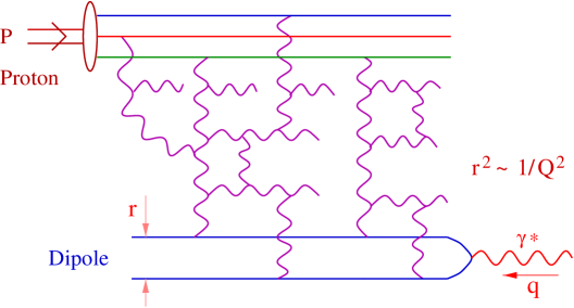
Figure 1: An instantaneous gluon configuration in the proton wavefunction as ‘seen’ in DIS at small $x$.

The first process, Fig. 2.a, represents one step in the standard BFKL evolution $\!{}^{{\bf?}}$; by iterating this step, one generates gluon ladders which are resummed in the solution to the BFKL equation $\!{}^{{\bf?}}$. By itself, this mechanism entails a rapid growth of the gluon distribution (exponential in $\tau$), which however leads to conceptual difficulties at very high energy : (i) The BFKL estimate for the dipole scattering amplitude $T_{\tau}(r)$ grows like a power of the energy, and thus eventually violates the unitarity bound $T_{\tau}(r)\leq 1$. (The upper limit $T_{\tau}=1$ corresponds to the ‘black disk’ limit, in which the dipole is totally absorbed by the target.) (ii) The BFKL ladder is not protected from deviations towards the non–perturbative domain at low transverse momenta $k_{\perp}^{2}\mathrel{\hbox to0.0pt{\raise 2.20013pt\hbox{$<$}\hss}{\lower 2.20013pt\hbox{$\sim$}}}\Lambda_{{\rm QCD}}^{2}$ (‘infrared diffusion’). With increasing energy, the BFKL solution receives larger and larger contributions from such soft intermediate gluons, and thus becomes unreliable.

These ‘small–$x$ problems’ of the BFKL evolution are both cured by gluon saturation $\!{}^{{\bf?}}$, the mechanism leading to the formation of a CGC: At sufficiently high energy, when the gluon density in the target becomes very large, the $n\to 2$ recombination processes illustrated in Fig. 2.b start to be important and tame the growth of the gluon distribution. Such processes are included (to all orders) in the JIMWLK equation $\!{}^{{\bf?},{\bf?},{\bf?}}$, a non–linear and functional generalization of the BFKL equation which describes the evolution of the ensemble of gluon correlations in the approach towards saturation. (As manifest on Fig. 2.b, the standard ‘gluon distribution’, which is a 2–point function, gets coupled to the higher $n$–point functions via the recombination effects.) Remarkably, the JIMWLK equation is a (functional) Fokker–Planck equation, which describes the high–energy evolution as a classical stochastic process $\!{}^{{\bf?}}$ — a random walk in the functional space of gluon fields. When applied to scattering amplitudes for simple external projectiles (like color dipoles, quadrupoles, etc.), the JIMWLK equation generates an infinite set of coupled evolution equations that were originally derived by Balitsky $\!{}^{{\bf?}}$.

(a)                                 (b)                                   (c)

Figure 2: Gluon processes which occur in one step of high energy evolution.

However, as recently noticed in Ref. $\!{}^{{\bf?}}$, the Balitsky–JIMWLK hierarchy misses the $2\to n$ splitting processes illustrated in Fig. 2.c, which describe the bremsstrahlung of additional small–$x$ gluons in one step of the evolution. By themselves, such processes are important in the dilute regime at relatively low energy (or, for a given energy, at relatively high transverse momenta $k_{\perp}\gg Q_{s}$), where they generate the $n$–point correlation functions with $n>2$ from the dominant 2–point function (the gluon distribution). But once generated, the higher $n$–point functions are rapidly amplified by their subsequent BFKL evolution (the faster the larger is $n$) and eventually play an important role in the non–linear dynamics leading to saturation. Thus, such splitting processes are in fact important for the evolution towards high gluon density, as first observed in numerical simulations $\!{}^{{\bf?}}$ of Mueller’s ‘dipole picture’ $\!{}^{{\bf?}}$ and recently explained in Refs. $\!{}^{{\bf?},{\bf?},{\bf?}}$.

3 QCD scattering amplitudes from statistical physics

Equations including both merging and splitting in the limit where the number of colors $N_{c}$ is large have recently became available $\!{}^{{\bf?}}$, but these are still quite complicated and their exploration is only at the beginning (see my next presentation $\!{}^{{\bf?}}$). Still, as we shall argue now, the asymptotic behaviour of the corresponding solutions — where by ‘asymptotic’ we mean both the high–energy limit $\tau\to\infty$ and the weak coupling limit $\alpha_{s}\to 0$ — can be a priori deduced from universality considerations relating high–energy QCD to problems in statistical physics $\!{}^{{\bf?}}$.

To that aim, it is convenient to rely on the event–by–event description $\!{}^{{\bf?}}$ of the scattering between the external dipole and the hadronic target, and to use the large–$N_{c}$ approximation to replace the gluons in the target wavefunction by color dipoles $\!{}^{{\bf?}}$ (which is indeed correct in the dilute regime). Then, the scattering amplitude in a given event can be estimated as

$$T_{\tau}(r,b)\,\simeq\,\alpha_{s}^{2}\,f_{\tau}(r,b)\,,$$ (1)

where $\alpha_{s}^{2}$ is the scattering amplitude between two dipoles with comparable sizes and nearby impact parameters, and $f_{\tau}(r,b)$ is the occupation number for target dipoles with size $r$ at impact parameter $b$. Since, clearly, $f$ is a discrete quantity: $f=0,1,2,\dots$, so is also the scattering amplitude in a given event: $T$ is a multiple integer of $\alpha_{s}^{2}$. The estimate (1) is based on the single scattering approximation, and thus is valid in the dilute target regime, where $T\ll 1$.

In this dipole language, the $2\to 4$ gluon splitting depicted in Fig. 2.c is tantamount to $1\to 2$ dipole splitting, and generates fluctuations in the dipole occupation number and hence in the scattering amplitude. Thus, the evolution of the amplitude $T_{\tau}(r,b)$ with increasing $\tau$ represents a stochastic process characterized by an expectation value $\langle T(r,b)\rangle_{\tau}\simeq\alpha_{s}^{2}\,\langle f(r,b)\rangle_{\tau}$, and also by fluctuations $\delta T\sim\alpha_{s}^{2}\delta f\sim\sqrt{\alpha_{s}^{2}T}$, where we have used the fact that $\delta f\sim\sqrt{f}$ for fluctuations in the particle number. These fluctuations are relatively important (in the sense that $\delta T\mathrel{\hbox to0.0pt{\raise 2.20013pt\hbox{$>$}\hss}{\lower 2.20013pt\hbox{$\sim$}}}T$) only in the very dilute regime where $\langle f\rangle\mathrel{\hbox to0.0pt{\raise 2.20013pt\hbox{$<$}\hss}{\lower 2.20013pt\hbox{$\sim$}}}1$, or $\langle T\rangle\mathrel{\hbox to0.0pt{\raise 2.20013pt\hbox{$<$}\hss}{\lower 2.20013pt\hbox{$\sim$}}}\alpha_{s}^{2}$.

3.1 The mean field approximation (BK, FKPP & geometric scaling)

Unitarity corrections in the form of multiple scattering start to be important when $T\sim 1$; according to Eq. (1), this happens for dipole occupation numbers of order $1/\alpha_{s}^{2}$. Consider first the formal limit $\alpha_{s}^{2}\to 0$, in which the maximal occupation number $N\sim 1/\alpha_{s}^{2}$ becomes arbitrarily large. Then one can neglect the particle number fluctuations and follow the evolution of the scattering amplitude in the mean field approximation (MFA). This is described by the BK equation $\!{}^{{\bf?},{\bf?}}$, a non–linear version of the BFKL equation which, mediating some approximations, can be shown $\!{}^{{\bf?}}$ to be equivalent to the FKPP equation $\!{}^{{\bf?}}$. The latter represents the MFA for the reaction–diffusion process $A\rightleftharpoons A+A$ and related phenomena in biology, chemistry, astrophysics, etc. (see $\!{}^{{\bf?}}$ for recent reviews and more references), and reads

$$\partial_{\tau}T(\rho,\tau)\,=\,\partial_{\rho}^{2}T(\rho,\tau)\,+\,T(\rho,\tau)\,-\,T^{2}(\rho,\tau),$$ (2)

in notations appropriate for the QCD problem at hand: $T(\rho,\tau)\equiv\langle T(r)\rangle_{\tau}$ and $\rho\equiv\ln(r_{0}^{2}/r^{2})$, with $r_{0}$ a scale introduced by the initial conditions at low energy. Note that weak scattering ($T\ll 1$) corresponds to small dipole sizes ($r\ll 1/Q_{s}$), and thus to large values of $\rho$. In momentum space, $\rho\sim\ln k_{\perp}^{2}$. The three terms on the r.h.s. of Eq. (2) describe, respectively, diffusion, growth and recombination. Together, the first two terms represent an approximate version of the BFKL dynamics, while the latter is the non–linear term which describes multiple scattering and ensures that the evolution is consistent with the unitarity bound $T\leq 1$. In fact, $T=1$ is clearly the high–energy limit of the solution to Eq. (2).

The solution $T_{\tau}(\rho)$ to Eq. (2) is a front which interpolates between two fixed points : the stable fixed point $T=1$ (the unitarity limit) at $\rho\to-\infty$, and the unstable fixed point $T=0$ at $\rho\to\infty$ (see Fig. 3). The position of the front, which marks the transition between strong and weak scattering, defines the saturation scale : $\rho_{s}(\tau)\equiv\ln(r_{0}^{2}Q_{s}^{2}(\tau))$. With increasing $\tau$, the front moves towards larger values of $\rho$, as illustrated in Fig. 3.

The dominant mechanism for front propagation is the BFKL growth in the tail of the distribution at large $\rho$ : the front is pulled by the rapid growth of a small perturbation around the unstable state $\!{}^{{\bf?}}$. In view of that, the velocity of the front $\lambda\equiv{d\rho_{s}}/{d\tau}$ is fully determined by the linearized version of Eq. (2) (i.e., the BFKL equation), which describes the dynamics in the tail. By solving the BFKL equation one finds $\!{}^{{\bf?},{\bf?}}$ that, for $\rho>\rho_{s}(\tau)$ and sufficiently large $\tau$,

$$T_{\tau}(\rho)\,\simeq\,{\rm e}^{\omega\bar{\alpha}_{s}\tau}\,{\rm e}^{-\gamma\rho}\,=\,{\rm e}^{-\gamma(\rho-\rho_{s}(\tau))}\,,\qquad\rho_{s}(\tau)\equiv c\bar{\alpha}_{s}\tau,$$ (3)

where $\bar{\alpha}_{s}={\alpha}_{s}N_{c}/\pi$, $\gamma=0.63..$, and $c\equiv\omega/\gamma=4.88..\,$. From Eq. (3) one can immediately identify the velocity of the front in the MFA as $\lambda_{0}=c\bar{\alpha}_{s}$. Since $Q_{s}^{2}(\tau)\simeq Q_{0}^{2}\,{\rm e}^{\lambda_{0}\tau}$, it is furthermore clear that $\lambda_{0}$ plays also the role of the saturation exponent (here, in the MFA).

According to Eq. (3), the scattering amplitude depends only upon the difference $\rho-\rho_{s}(\tau)$ : $T_{\tau}(\rho)={\cal A}\big{(}\rho-\rho_{s}(\tau)\big{)}$. This is an exact property of the FKPP equation (at sufficiently large $\tau$) and expresses the fact that the corresponding front is a traveling wave which propagates without distortion $\!{}^{{\bf?}}$. In QCD, this property is valid only within a limited range, namely for $\!{}^{{\bf?}}$

$$0\,<\,\rho-\rho_{s}(\tau)\,\mathrel{\hbox to0.0pt{\raise 2.20013pt\hbox{$<$}\hss}{\lower 2.20013pt\hbox{$\sim$}}}\,\rho_{s}(\tau)\,$$ (4)

(the “geometric scaling window”; see below), because of the more complicated non—locality of the BFKL, or BK, equations. When translated to the original variables $r$ and $\tau$, this property implies that the dipole amplitude scales as a function of $r^{2}Q_{s}^{2}(\tau)$ : $\langle T(r)\rangle_{\tau}\approx{\cal A}\big{(}r^{2}Q_{s}^{2}(\tau)\big{)}$. This is the property originally referred to as geometric scaling $\!{}^{{\bf?},{\bf?},{\bf?}}$, and which might explain a remarkable regularity observed $\!{}^{{\bf?}}$ in the small–$x$ data for DIS at HERA. Namely, for $x\leq 0.01$, the total cross–section $\sigma_{\gamma^{*}p}(x,Q^{2})$ for the absorbtion of the virtual photon shows approximate scaling as a function of $Q^{2}/Q_{s}^{2}(x)$, with $Q_{s}^{2}(x)\propto(1/x)^{\lambda}$ and $\lambda\approx 0.3$ from a fit to the data. This measured value of $\lambda$ is quite far away from the above prediction $\lambda_{0}=c\bar{\alpha}_{s}\sim 1$ of the BFKL equation; but after including the NLO corrections to the BFKL equation (see Ref. $\!{}^{{\bf?}}$ for details), the ensuing, improved, theoretical prediction $\!{}^{{\bf?}}$ decreases indeed to a value close to 0.3.

Figure 3: Evolution of the continuum front of the Balitsky–Kovchegov equation with increasing $\tau$.

3.2 The effects of fluctuations

What is the validity of the mean field approximation ? We have earlier argued that the gluon splitting processes (cf. Fig. 2.c) responsible for dipole number fluctuations should play an important role in the dilute regime. This is further supported by the above considerations on the pulled nature of the front: Since the propagation of the front is driven by the dynamics in its tail where the fluctuations are a priori important, the front properties should be strongly sensitive to fluctuations. This is indeed known to be the case for the corresponding problem in statistical physics $\!{}^{{\bf?},{\bf?}}$, as it can be understood from the following, qualitative, argument:

Consider a particular realization of the stochastic evolution of the target, and the corresponding scattering amplitude, which is discrete (in steps of $\alpha_{s}^{2}$). Because of discreteness, the microscopic front looks like a histogram and thus is necessarily compact : for any $\tau$, there is only a finite number of bins in $\rho$ ahead of $\rho_{s}$ where $T_{\tau}$ is non–zero (see Fig. 4). This property has important consequences for the propagation of the front. In the empty bins on the right of the tip of the front, the local, BFKL, growth is not possible anymore (as this would require a seed). Thus, the only way for the front to progress there is via diffusion, i.e., via radiation from the occupied bins at $\rho<\rho_{\rm tip}$ (compare in that respect Figs. 3 and 4). But since diffusion is less effective than the local growth, we expect the velocity of the microscopic front (i.e., the saturation exponent) to be reduced as compared to the respective prediction of the MFA.

Figure 4: Evolution of the discrete front of a microscopic event with increasing rapidity $\tau$. The small blobs are meant to represent the elementary quanta $\alpha_{s}^{2}$ of $T$ in a microscopic event.

To obtain an estimate for this effect $\!{}^{{\bf?},{\bf?}}$, we shall rely on the universality of the dominant asymptotic ($\tau\to\infty$ and $N\equiv 1/\alpha_{s}^{2}\gg 1$) behaviour, which has been observed in the context of statistical physics and justified by Brunet and Derrida $\!{}^{{\bf?}}$ through the following, intuitive, argument: For a given microscopic front and $N\gg 1$, the MFA should work reasonably well everywhere except in the vicinity of the tip of the front, where the occupation number $f$ becomes of order one and the linear growth term becomes ineffective. (Note that, in QCD, $f\sim 1$ corresponds to $T\sim\alpha_{s}^{2}$, which is precisely where one expects the fluctuation effects to become important.) Accordingly, Brunet and Derrida suggested a modified version of the FKPP equation (2) in which the ‘BFKL–like’ growth term is switched off when $T<\alpha_{s}^{2}$ :

$$\partial_{\tau}T(\rho,\tau)\,=\,\partial_{\rho}^{2}T\,+\,\Theta\big{(}T-\alpha_{s}^{2}\big{)}T(1-T).$$ (5)

By solving this equation in the linear regime, they have obtained the first correction to the front velocity as compared to the MFA (in notations adapted to QCD; see Ref. $\!{}^{{\bf?}}$ for details):

$$\lambda\,\simeq\,\bar{\alpha}_{s}\left[c\,-\,\frac{\kappa}{\ln^{2}(1/\alpha_{s}^{2})}\,+\,{\cal O}\big{(}1/\ln^{3}\alpha_{s}^{2}\big{)}\right]\,,$$ (6)

where the numbers $c\approx 4.88$ and $\kappa\approx 150$ are fully determined by the linear (BFKL) equation. In QCD, the same result has been first obtained through a different but related argument by Mueller and Shoshi $\!{}^{{\bf?}}$. Note the extremely slow convergence of this result towards its mean field limit: the corrective term vanishes only logarithmically with decreasing $1/N=\alpha_{s}^{2}$, rather than the power–like suppression usually found for the effects of fluctuations. This is related to the high sensitivity of the pulled fronts to fluctuations, as alluded to above. The merely logarithmic dependence of Eq. (6) upon the value of the cut–off also explains its universality: a renormalization $\alpha_{s}^{2}\to A\alpha_{s}^{2}$ of the latter does not change the dominant correction in Eq. (6).

But although it becomes an exact result in QCD in the formal limit $\alpha_{s}^{2}\to 0$, the estimate in Eq. (6) is clearly useless for any practical application, because of the very slow convergence of the expansion there. Still, this has the merit to demonstrate that the effects of the fluctuations are potentially large, which invites us to critically reexamine the results previously obtained from the BK equation. In fact, from the correspondence with statistical physics, we also know $\!{}^{{\bf?}}$ that the geometric scaling property of the BK solution will be eventually washed out by fluctuations at sufficiently high energy. But in order to understand how fast this actually happens (i.e., up to what energy one should expect geometric scaling to be a good property), and also to estimate the saturation exponent for realistic values of $\alpha_{s}$, one needs to solve the actual evolution equations in QCD at large–$N_{c}$ $\!{}^{{\bf?},{\bf?}}$, to be described in my next contribution to these Proceedings $\!{}^{{\bf?}}$.

References

- [1] E. Iancu and A.H. Mueller, Nucl. Phys. A730 (2004) 494.
- [2] A.H. Mueller and A.I. Shoshi, Nucl. Phys. B692 (2004) 175.
- [3] S. Munier and R. Peschanski, Phys. Rev. Lett. 91 (2003) 232001.
- [4] E. Iancu, A.H. Mueller and S. Munier, Phys. Lett. B606 (2005) 342.
- [5] E. Iancu and D.N. Triantafyllopoulos, Nucl. Phys. A756 (2005) 419; Phys. Lett. B610 (2005) 253.
- [6] I. Balitsky, Nucl. Phys. B463 (1996) 99.
- [7] J. Jalilian-Marian, A. Kovner, A. Leonidov, H. Weigert, Nucl. Phys. B504 (1997) 415; Phys.Rev. D59 (1999) 014014; J. Jalilian-Marian, A. Kovner, H. Weigert, Phys.Rev. D59 (1999) 014015; A. Kovner, J.G. Milhano, H. Weigert, Phys.Rev. D62 (2000) 114005.
- [8] E. Iancu, A. Leonidov, L. McLerran, Nucl. Phys. A692 (2001) 583; Phys. Lett. B510 (2001) 133; E. Ferreiro, E. Iancu, A. Leonidov, L. McLerran, Nucl. Phys. A703(2002)489.
- [9] H. Weigert, Nucl. Phys. A703 (2002) 823.
- [10] A.H. Mueller, Nucl. Phys. B415 (1994) 373; ibid. B437 (1995) 107.
- [11] G.P. Salam, Nucl. Phys. B449 (1995) 589; ibid. B461 (1996) 512.
- [12] E. Iancu and A.H. Mueller, Nucl. Phys. A730 (2004) 460.
- [13] L. McLerran and R. Venugopalan, Phys. Rev. D49 (1994) 2233; ibid. 49 (1994) 3352.
- [14] Yu.V. Kovchegov, Phys. Rev. D60 (1999), 034008; ibid. D61 (1999), 074018.
- [15] R.A. Fisher, Ann. Eugenics 7 (1937) 355; A. Kolmogorov, I. Petrovsky, and N. Piscounov, Moscou Univ. Bull. Math. A1 (1937) 1.
- [16] A.M. Stasto, K. Golec-Biernat and J. Kwiecinski, Phys. Rev. Lett. 86 (2001) 596.
- [17] E. Iancu, K. Itakura, and L. McLerran, Nucl. Phys. A708 (2002) 327.
- [18] W. Van Saarloos, Phys. Rep. 386 (2003) 29; D. Panja, ibid. 393 (2004) 87.
- [19] E. Brunet and B. Derrida, Phys. Rev. E56 (1997) 2597.
- [20] A.H. Mueller and D.N. Triantafyllopoulos, Nucl. Phys. B640 (2002) 331.
- [21] D.N. Triantafyllopoulos, Nucl. Phys. B648 (2003) 293.
- [22] A.H. Mueller, A.I. Shoshi, S.M.H. Wong, Nucl. Phys. B715 (2005) 440.
- [23] J.-P. Blaizot, E. Iancu, K. Itakura, D.N. Triantafyllopoulos, Phys. Lett. B615 (2005) 221.
- [24] A. Kovner and M. Lublinsky, Phys. Rev. D71 (2005) 085004; Phys. Rev. Lett. 94 (2005) 181603; arXiv:hep-ph/0503155; arXiv:hep-ph/0510047.
- [25] Y. Hatta, E. Iancu, L. McLerran, A. Stasto, D.N. Triantafyllopoulos, hep-ph/0504182.
- [26] C. Marquet, A.H. Mueller, A.I. Shoshi, and S.M.H. Wong, arXiv:hep-ph/0505229.
- [27] Y. Hatta, E. Iancu, L. McLerran, and A. Stasto, arXiv:hep-ph/0505235.
- [28] I. Balitsky, arXiv:hep-ph/0507237.
- [29] E. Iancu, these proceedings, arXiv:hep-ph/0510265.
- [30] L.N. Lipatov, Sov. J. Nucl. Phys. 23 (1976) 338; E.A. Kuraev, L.N. Lipatov and V.S. Fadin, Zh. Eksp. Teor. Fiz 72, 3 (1977) (Sov. Phys. JETP 45 (1977) 199); Ya.Ya. Balitsky and L.N. Lipatov, Sov. J. Nucl. Phys. 28 (1978) 822.
- [31] L.V. Gribov, E.M. Levin, and M.G. Ryskin, Phys. Rept. 100 (1983) 1; A.H. Mueller and J. Qiu, Nucl. Phys. B268 (1986) 427.
- [32] J.-P. Blaizot, E. Iancu and H. Weigert, Nucl. Phys. A713 (2003) 441.