Abstract

We use the detection of neutrinos from a future galactic type-II supernova event in a water Cerenkov detector like Super-Kamiokande to constrain the possible violation of spin-statistics by neutrinos resulting in their obeying a mixed statistics instead of Fermi-Dirac.

Keywords: supernova neutrinos, neutrino properties

^⋆ email: sandhya@thphys.ox.ac.uk

^† email: kamales.kar@saha.ac.in

Recently there was a suggestion of neutrinos violating the spin-statistics relation and thereby becoming a good candidate for all (or part) of the dark matter in the universe [1]. There are a number of papers which discuss the possible violation of spin-statistics relation by neutrino though no consistent satisfactory model exists [2, 3, 4, 5]. On the other hand the experimental verification of neutrinos with half spin following a mixed statistics was not thoroughly studied earlier. For nucleons however such studies exist [2]. The recent paper on the possibility of neutrinos violating the Pauli Exclusion Principle [1] however has renewed interest in the subject [6]. The Doglov-Smirnov work [1] points out that if neutrinos do obey Bose-Einstein (BE) statistics instead of Fermi-Dirac (FD), then they may form large cosmological Bose condensates and account for the dark matter. This also opens up the possibility of large lepton asymmetry in the universe. As double beta decay disallows purely bosonic neutrinos, one will be interested in mixed statistics in terms of a continuous “Fermi-Bose” parameter, $\kappa$ ($\kappa=-1$ is purely fermionic and $\kappa=1$ is purely bosonic) [7]. This on the other hand has astrophysical consequences as well. For example this will have impact on the type II supernova (SN) dynamics and will change the energy spectrum of neutrinos coming out of the supernova. In this report we shall not be concerned with the justification of the Dolgov-Smirnov suggestion but concentrate on the question: Given the scenario of neutrinos of all three flavors obeying the mixed statistics, how would future observation of galactic neutrinos in large terrestrial detectors put limits on the mixed statistics parameter $\kappa$. We assume that apart from (possibly) violating the spin-statistics theorem, the massive neutrinos do not have any other non-standard property. We shall see that with detectors like Super-Kamiokande (SK) one indeed can test this hypothesis at a significant level of accuracy.

Massive stars at the end of their normal lifespan, collapse due to the gravitational pull once the silicon burning in the core stops and the core has a mass greater than the Chandrasekhar mass. The neutrinos that are produced by electron capture on nuclei and free protons during the initial collapse phase escape. However, as the density of the core exceeds densities of $10^{11}-10^{12}$ gm/cc during collapse, neutrinos get trapped. At densities higher than the nuclear matter density a shock wave forms inside the core and travels outward. Whether the shock wave can reach the edge of the core with enough energy to cause the explosion with the observed energies is the central question of supernova physics today.

At the high densities and temperatures of the SN core during the post-bounce phase, neutrinos and antineutrinos of all three flavors are produced. Almost $\sim 99\%$ of the gravitational energy produced through the huge contraction of the star ($\sim$ a few times $10^{53}$ ergs) is released in the form of the six species of neutrinos ($\nu_{e}$, $\nu_{\mu}$, $\nu_{\tau}$ and their antiparticles). In the high density central part of the core, neutrinos of each flavor have high opacity and hence cannot come out. But at larger radius due to a strong density gradient, neutrinos can diffuse out and eventually escape. Therefore, we expect almost thermal spectra for all the neutrino species, with temperatures characteristic of their radius of last scattering in the SN, usually called the neutrino sphere radius. Since ${\nu_{e}}$ and ${\bar{\nu}_{e}}$ have charged current interactions with the SN matter in addition to neutral current interactions and since SN matter is neutron rich, ${\nu_{e}}$, ${\bar{\nu}_{e}}$ and $\nu_{x}$ (’x’ stands for $\mu$, $\tau$, $\bar{\mu}$ and $\bar{\tau}$) decouple at different radii. Hence the neutrino spheres of the three different types, $\nu_{e}$, $\bar{\nu}_{e}$ and $\nu_{x}$, have different radii and hence different equilibrium temperatures ($T_{\nu}$), with $T_{\nu_{e}}<T_{\bar{\nu}_{e}}<T_{\nu_{x}}(T_{x})$. For our purpose we shall take $T_{\nu_{e}}=3.5$ MeV, $T_{\bar{\nu}_{e}}=5$ MeV and $T_{\nu_{x}}=8$ MeV [8], used in most simulations and calculations as the standard values. As there are arguments which claim that $T_{\bar{\nu}_{e}}$ and $T_{\nu_{x}}$ should be closer [9], we vary these temperatures over a range as detailed later in this report. These temperatures are obtained by using FD equilibrium energy distributions and may change somewhat had the simulations been carried out with BE distributions or distributions with mixed statistics. However the qualitative results of our investigation here will not change if they are done with equilibrium BE temperatures for $\nu_{e}$, $\bar{\nu}_{e}$ and $\nu_{x}$. Again realistic simulations indicate small departures from equilibrium distribution of energies of the neutrino, with the high energy tail lower or “pinched”. The pinching factor is expected to range between $\eta_{e}\sim 0-3$, $\eta_{\bar{e}}\sim 0-3$ and $\eta_{x}\sim 0-2$ for the ${\nu_{e}}$, ${\bar{\nu}_{e}}$ and $\nu_{x}$ flux respectively [10]. We further assume that the total luminosity $E_{B}$ is equipartitioned among the six neutrino and antineutrino species. We remind readers here that the electron type antineutrinos (with at most one neutrino scattering event) were detected alongwith the SN 1987A explosion. But with 11 and 8 events at Kamioka and IMB, fitting of energy spectrum and determination of temperature had large errors [11].

Following [1] we parametrize the equilibrium distribution of the neutrinos with a mixed statistics as

$$f^{(eq)}_{\nu}=({\rm exp}(E/T)+\kappa)^{-1}~{},$$ (1)

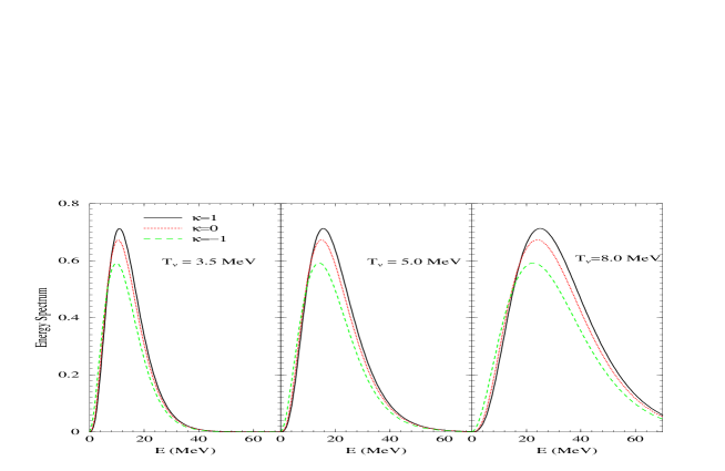
where $E$ is the energy of the neutrinos, $T$ the temperature of the distribution and $\kappa$ is the Fermi-Bose parameter for the mixed statistics, as mentioned earlier. Fig. 1 shows the energy spectrum of the neutrinos corresponding to FD ($\kappa=+1$), Maxwell Boltzmann MB ($\kappa=0$) and BE ($\kappa=-1$) distributions, with typical temperatures of 3.5 (left panel), 5 (middle panel) and 8 MeV (right panel). The area under each of the curves gives the average energy expected for the corresponding values of $T_{\nu}$ and $\kappa$. It is clear from the figure that for the same $T_{\nu}$, at small values of $E$ the predicted spectrum for the BE distribution is higher than for the FD distribution. However for large $E$, the trend is reversed and the spectrum predicted for FD is higher than that for the BE distribution and has a longer high energy tail. This trend reflects the fact that for the same $T_{\nu}$, the predicted average energy for the neutrinos is larger for the FD distribution. We also stress from Fig. 1 the fact that the spectral shape for the FD and BE distributions are different. We want to use the signature of this difference in predicted average energy and spectral shape of the SN neutrinos in terrestrial detectors, to disfavor the “wrong” neutrino statistical distribution and put limits on the Fermi-Bose parameter $\kappa$.

In Fig. 2 we show the effect of introducing the pinching in the FD distribution. We plot the galactic SN neutrino flux spectrum expected at earth given by [10]

$$F_{\alpha}^{0}=\frac{L_{\alpha}}{4\pi D^{2}T_{\alpha}^{4}F_{3}(\eta_{\alpha})}\frac{E^{2}}{({\rm exp}(E/T_{\alpha}-\eta_{\alpha})+\kappa)}~{},$$ (2)

where $L_{\alpha}$ is the SN luminosity released in $\nu_{\alpha}$, $D$ is the distance of the SN (10 kpc), $\eta_{\alpha}$ is the pinching factor and

$$F_{3}(\eta_{\alpha})=\int_{0}^{\infty}\frac{x^{3}}{{\rm exp}(x-\eta_{\alpha})+\kappa}dx~{}.$$ (3)

The black solid line shows the spectrum for a pure FD distribution with $\eta_{\alpha}=0$, the red dotted line corresponds to a pinched FD distribution with $\eta_{\alpha}=2$ while the green dot-dashed line is for the pure BE distribution. All the three spectra plotted in the figure have the same average energy. A comparison of the three spectra shows that the difference in the spectral shape between the BE and FD distribution increases as $\eta_{\alpha}$ changes from zero. Hence, we expect it would be easiest to confuse between the BE and FD distributions when $\eta_{\alpha}=0$ and it is for this case that we generally expect the minimum $\chi^{2}$. Since we want to check how well one can differentiate between the FD and BE (and mixed) distributions and since this seems to be most difficult for the pure FD distribution, we will neglect the effect of pinching in the spectrum in the rest of the paper for simplicity.

We shall be concerned with the large water Cerenkov detectors like SK. The main interaction channel in SK which is important for the detection of the SN neutrinos is the charged current capture of $\bar{\nu}_{e}$ on free protons:

$$\bar{\nu}_{e}+p\rightarrow e^{+}+n$$ (4)

with a threshold ${\bar{\nu}_{e}}$ energy of 1.3 MeV. The number of positrons expected in SK from a galactic SN explosion is given by

$$R=N\int dE_{A}\int dE_{T}~{}R(E_{A},E_{T})\int dE~{}\sigma_{{\bar{\nu}_{e}}p}(E)~{}\Big{[}F_{\bar{e}}(E)~{}P_{\bar{e}\bar{e}}(E)+F_{\bar{x}}(E)(1-P_{\bar{e}\bar{e}}(E))\Big{]}~{},$$ (5)

where N is the number of target protons and $\sigma_{{\bar{\nu}_{e}}p}$ is the ${\bar{\nu}_{e}}$-$p$ capture cross-sections. $E$ is the energy of the incident ${\bar{\nu}_{e}}$, while $E_{A}$ and $E_{T}$ are respectively the measured and true energy of the emitted positron. The true and measured energy of the positron are related through $R(E_{A},E_{T})$, the Gaussian energy resolution function of the detector given by,

$$R(E_{A},E_{T}) = \frac{1}{\sqrt{2\pi\sigma_{0}^{2}}}\exp\left(-\frac{(E_{A}-E_{T})^{2}}{2\sigma_{0}^{2}}\right)~{},$$ (6)

where we assume $\sigma_{0}$ to have a value similar to what is used in the analysis of the SK solar neutrino data. $F_{\bar{e}}$ and $F_{\bar{x}}$ are the flux of ${\bar{\nu}_{e}}$ and $\bar{\nu}_{x}$ produced in the SN core and depend on the spin statistics of the neutrinos and $P_{\bar{e}\bar{e}}$ is the survival probability of the SN ${\bar{\nu}_{e}}$.

Before reaching the detector, the neutrinos travel through the SN matter, propagate through vacuum and finally may even travel through earth matter depending on the time of the SN burst. For the range of neutrino oscillation parameters consistent with the solar and KamLAND reactor data ($\Delta m^{2}_{\odot}\equiv\Delta m^{2}_{21}=8.0\times 10^{-5}$ eV² and $\sin^{2}\theta_{\odot}\equiv\sin^{2}\theta_{12}=0.31$ [12, 13]) and SK atmospheric data ($\Delta m^{2}_{\rm atm}\equiv\Delta m^{2}_{31}=2.1\times 10^{-3}$ eV² and $\sin^{2}2\theta_{\rm atm}\equiv\sin^{2}2\theta_{23}=1.0$ [14]), one expects large matter enhanced oscillation inside the supernova and possible regeneration effects inside the earth [10, 15]. As a result, the more energetic $\bar{\nu}_{\mu}$ and $\bar{\nu}_{\tau}$ get converted to $\bar{\nu}_{e}$ and make the spectra harder. This results in enhancing the number of expected charged current events in the detector and is incorporated in our numerical analysis through $P_{\bar{e}\bar{e}}$ in Eq. (5). We assume that the supernova explodes at a distance of 10 kpc from us and that the time of the event is such that the neutrinos do not cross the earth matter. The survival probability $P_{\bar{e}\bar{e}}$ depends critically on the value of $\theta_{13}$, which at the moment has a very weak bound of $\sin^{2}\theta_{13}<0.04$ at $3\sigma$ [12, 16]. In what follows, we will assume that the true values of the oscillation parameters $\Delta m^{2}_{21}$, $\sin^{2}\theta_{12}$ and $\Delta m^{2}_{31}$ have been determined with sufficient accuracy to the values mentioned above (see [17] and [18] for recent detailed discussions). For the major part of the paper, we will also assume that the true value of mixing angle $\theta_{13}\sim 0$. We will discuss the impact of the uncertainty on this oscillation parameter towards the end.

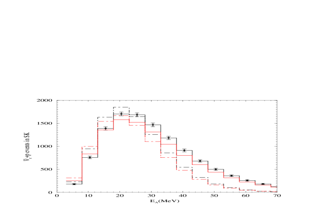
Fig. 3 displays the distribution of the number of $(\bar{\nu}_{e}+p)$ events in SK as a function of the measured energy $E_{A}$ of the positron. The black solid (dashed) line gives the event spectrum for a FD distribution with (without) neutrinos oscillations, while the red solid (dashed) line gives the expected event spectrum for a BE distribution. We assume $T_{\bar{\nu}_{e}}=5$ MeV, $T_{x}=8$ MeV and $E_{B}=3\times 10^{53}$ ergs. From the figure, BE distribution can be seen to underpredict the number of events over a large range of energy from about 12-70 MeV, compared to FD distribution. We also give the $\pm 1\sigma$ error bars corresponding to the number of events SK would observe in each bin for the FD distribution. This clearly shows that a large detector like SK should be able to distinguish between the different statistics at a good confidence level.

In order to quantify our statement, we perform a statistical analysis of the neutrino induced positron spectrum that SK would observe in the event of a galactic SN explosion. For the errors we take a Gaussian distribution and define our $\chi^{2}$ as

$$\chi^{2}=\sum_{i,j}(N_{i}^{theory}-N_{i}^{obsvd})(\sigma_{ij}^{2})^{-1}(N_{j}^{theory}-N_{j}^{obsvd})~{},$$ (7)

where $N_{i}^{theory}$ ($N_{i}^{obsvd}$) are the number of predicted (observed) events in the $i^{th}$ energy bin and the sum is over all bins. The error matrix $\sigma_{ij}^{2}$ contains the statistical and systematic errors. The systematic uncertainty will be eventually determined by the experimental collaboration after a real SN event has been observed in SK. However, for the moment we have simply assumed a 5% systematic uncertainty in the simulated “data”, fully correlated in all the bins. The number of energy bins used in our analysis is shown in Fig. 3. The $\chi^{2}$ function is minimized with respect to the parameters in the theory to give us a handle on the C.L. with which observation of SN neutrinos in SK could lead to the determination of their correct distribution function. In what follows, there are two kinds of statistical tests that we shall perform. In one, we shall compare the data set obtained for (say) the true FD distribution with the predicted event spectrum for the false BE distribution. This will give us the measure of the C.L. with which the false BE distribution could be ruled out. In another, we will compare the data set generated for (say) the true FD distribution ($\kappa=1$) and compare it with a distribution for all possible values of $\kappa$ in the range [$-1,1$], with $\kappa=-1$ corresponding to a pure BE distribution.

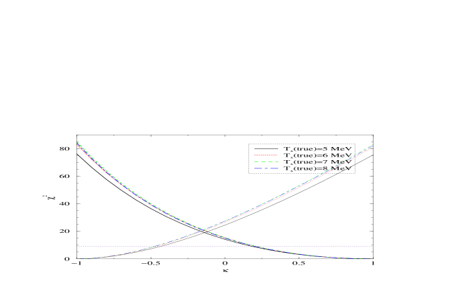
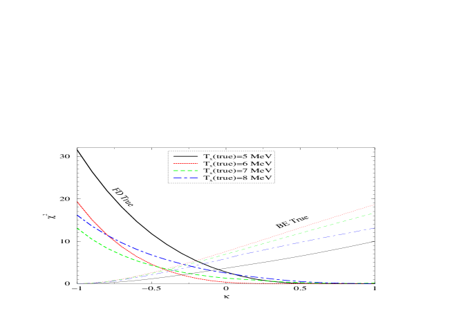
In Fig. 4 we show the $\chi^{2}$ as a function of the parameter $\kappa$. We assume that the only errors involved are experimental and keep all the theoretical inputs fixed. The thick lines show the $\chi^{2}$ for the case where the $N_{i}^{obsvd}$ correspond to $\kappa{\rm(true)}=1$ and hence to a “true” FD spectrum. The thin lines give the corresponding $\chi^{2}$ for the case when $\kappa{\rm(true)}=-1$ and the BE spectrum is true. For all the cases we generated the “data” for $T_{\bar{\nu}_{e}}{\rm(true)}=5$ MeV, while for $T_{x}{\rm(true)}$ we assume four different values displayed in the figure. If we define our $3\sigma$ limit as given by $\Delta\chi^{2}=9$, then the figure shows that for a true FD spectrum, SK could in principle restrict $\kappa>0.2$ at $3\sigma$, for $T_{\bar{\nu}_{e}}{\rm(true)}=5$ MeV and $T_{x}{\rm(true)}=8$ MeV. In particular, the false BE distribution ($\kappa=-1$) can be ruled out comprehensively at about $9\sigma$ level. If on the other hand BE distribution was true, then all $\kappa>-0.5$ could be ruled out at $3\sigma$ and the false FD distribution ($\kappa=1$) could be disfavored at about $9\sigma$ level.

In the discussion above we had assumed that all theoretical parameters involving the prediction of the SN neutrino fluxes were absolutely known. However, this is far from true. In fact, the error coming from our lack of correct modeling for the supernova neutrino energies and luminosities is much larger than the experimental errors. In the last few years it has been realized [9] that the nucleon bremsstrahlung $NN\rightarrow NN\nu_{x}\bar{\nu}_{x}$ as well as ${\nu_{e}}{\bar{\nu}_{e}}\rightarrow\nu_{x}\bar{\nu}_{x}$ along with its inverse reaction are important and were not included in the earlier simulations of the neutrino transport inside the supernova. While the first process reduces the difference between $T_{x}$ and $T_{\bar{\nu}_{e}}$, the second ones increase the $\nu_{x}$ luminosity. We note that these uncertainties could also be correlated. In what follows, we take into account the uncertainties on the predicted neutrino fluxes by keeping both the total luminosity $E_{B}$ and the temperatures $T_{\bar{\nu}_{e}}$ and $T_{x}$ completely unconstrained, thus allowing for all possible values for these parameters. This method therefore can be used to gauge the potential of SK to determine the true energy distribution of the SN neutrinos, irrespective of our (lack of) knowledge of the initial SN fluxes. Henceforth, we will distinguish between the “true” values of the parameters (denoted as $T_{\bar{\nu}_{e}}{\rm(true)}$ etc.) at which we generate our projected SN neutrino data set and the fitted values of those parameters (denoted as $T_{\bar{\nu}_{e}}$ etc.), obtained through the minimization of the $\chi^{2}$ function defined in Eq. (7).

Fig. 5 shows the $\chi^{2}$ as a function of $T_{\bar{\nu}_{e}}{\rm(true)}$ for three assumed values of $T_{x}{\rm(true)}$. The thick lines in the figure show the case where the “data” $N_{i}^{obsvd}$ is generated assuming a true FD distribution for $E_{B}{\rm(true)}=3\times 10^{53}$ ergs and values of $T_{\bar{\nu}_{e}}{\rm(true)}$ between 4.5-7 MeV and for three different values of $T_{x}{\rm(true)}$ = 6, 7 and 8 MeV shown by red dotted and green dashed and blue dot-dashed lines respectively. This data set is then fitted with $N_{i}^{theory}$ calculated using the wrong BE distribution and with $T_{\bar{\nu}_{e}}$, $T_{x}$ and $E_{B}$ allowed to take any possible value which gives the minimum $\chi^{2}$ in the fit. The thin lines in the figure show the corresponding minimum $\chi^{2}$ when the true distribution appearing in $N_{i}^{obsvd}$ is BE and the wrong distribution chosen in $N_{i}^{theory}$ is FD. We note from the figure that if FD is the true distribution, then the SN data set in SK can be used to rule out the possibility of neutrinos obeying the BE statistics at the $5\sigma$ level for $T_{\bar{\nu}_{e}}{\rm(true)}>4.8$, 5.0 and 5.2 MeV for $T_{x}{\rm(true)}=6$, 7 and 8 MeV respectively. If the BE distribution for the neutrinos was true, then the wrong FD statistics could be ruled out at $5\sigma$ for $T_{\bar{\nu}_{e}}{\rm(true)}>6.0$, 5.9 and 6.1 MeV, when $T_{x}{\rm(true)}=6$, 7 and 8 MeV respectively. The wrong distribution can be ruled out at more than $3\sigma$ for both cases for all plausible values of $T_{\bar{\nu}_{e}}$.

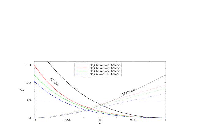
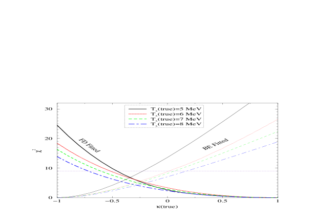
The C.L. with which any given value of $\kappa$ can be ruled out for either the case where FD (thick lines) or BE (thin lines) is the true distribution, can be seen from Fig. 6, where we have plotted the $\chi^{2}$ as a function of $\kappa$. For all the curves we take $T_{\bar{\nu}_{e}}{\rm(true)}=5$ MeV, while for $T_{x}{\rm(true)}$ we have assumed four values: 5 (black solid lines), 6 (red dotted lines), 7 (green dashed lines) and 8 (blue dot-dashed lines) MeV. The method of $\chi^{2}$ analysis is similar to that used for Fig. 5. In particular, for the case of true FD (BE) distribution shown by the thick (thin) lines, the data set $N_{i}^{obsvd}$ is generated for $\kappa{\rm(true)}=1$ ($\kappa{\rm(true)}=-1$), $E_{B}{\rm(true)}=3\times 10^{53}$ and the fixed values of $T_{\bar{\nu}_{e}}{\rm(true)}$ and $T_{x}{\rm(true)}$ mentioned above. This data set is then fitted with $N_{i}^{theory}$ calculated for each $\kappa$ in the range [$-1,1$], with the SN parameters allowed to vary freely. For the true FD distribution, we can limit allowed $\kappa>-0.39$, $-0.45$ and $-0.55$ at $3\sigma$, for $T_{x}{\rm(true)}=6$, 7 and 8 MeV respectively. For BE as the true distribution, $\kappa<0.13$, 0.21 and 0.38 is allowed at $3\sigma$, for $T_{x}{\rm(true)}=6$, 7 and 8 MeV respectively.

From the Fig. 6 we note that when a theoretical distribution with a wrong $\kappa$ is used to fit the data, the $\chi^{2}$ obtained for the true FD distribution is in general larger than that for the true BE distribution. This happens because by changing the (anti)neutrino temperatures and luminosity, a spectrum with mixed statistics can reproduce the data set more easily when the latter corresponds to a BE distribution. We have checked that the spectral shape is the most important factor in this case. Indeed if we analyzed the data set on total $({\bar{\nu}_{e}}+p)$ observed rate in SK rather than the positron energy spectrum, the sensitivity to $\kappa$ would get completely lost since the total rate can always be reproduced by a theory with any $\kappa$ when $E_{B}$, $T_{\bar{\nu}_{e}}$ and $T_{x}$ are allowed to vary freely.

Fig. 7 shows the $\chi^{2}$ we can expect when a data set corresponding to a particular case of mixed neutrino spin-statistics is fitted with either a pure FD or a pure BE distribution. We generate the data set corresponding to each of values of $-1<\kappa({\rm true})<1$ and fit it with either a theory with FD distribution (thick lines) or a theory with BE distribution (thin lines). We can draw similar inferences from this plot as obtained from Fig. 6.

Throughout our discussion so far we have played down the impact of the oscillation parameters. We generated our data set at the benchmark values of $\Delta m^{2}_{21}=8\times 10^{-5}$ eV², $\sin^{2}\theta_{12}=0.3$, $\Delta m^{2}_{31}=2.1\times 10^{-3}$ eV² and $\sin^{2}\theta_{13}=0$ and kept them fixed in the fit. For the current allowed range of neutrino oscillation parameters, the survival probability for the SN (anti)neutrinos depend on $\Delta m^{2}_{21}$ and $\sin^{2}\theta_{12}$ only for (anti)neutrinos crossing the earth. Since we assume that the position and time of the SN in the galactic center with respect to our detector SK will be such that neutrinos do not cross the earth matter, we are justified in keeping $\Delta m^{2}_{21}$ and $\sin^{2}\theta_{12}$ fixed at any value of their current allowed range. However, the oscillations inside the SN matter depend crucially on the values of $\Delta m^{2}_{31}$ and $\theta_{13}$ [15]. Most importantly, for a given value of $\theta_{13}$ ($>10^{-6}$), whether large flavor oscillations appear in the neutrino or the antineutrino channel is determined by the sign of $\Delta m^{2}_{31}$, i.e. the neutrino mass hierarchy. The sign of $\Delta m^{2}_{31}$ is typically expected to be determined using matter effects in the 1-3 channel. For very large values of $\theta_{13}$, synergies between the T2K and NO$\nu$A experiments could somewhat indicate the $sgn(\Delta m^{2}_{31})$ [20]. However, an unambiguous measurement would require either a beta beam facility or a neutrino factory [21]. Resonant matter effects in the 1-3 channel encountered by atmospheric neutrinos can be exploited to probe the neutrino hierarchy both in water Cerenkov and large magnetized iron calorimeter detectors [22]. Recently some novel ways of probing the mass hierarchy requiring very precise measurements and using the “interference terms” between the different oscillation frequencies have been proposed [23]. Neutrinoless double beta decay experiments have the potential to provide us with the neutrino mass hierarchy even for vanishing $\theta_{13}$ [24, 25]. The uncertainty on the value/limit on $\theta_{13}$ is also expected to reduce in the future. The upper limit could be improved further to $\sin^{2}\theta_{13}\ \raisebox{-1.72218pt}{\hbox to0.0pt{$\sim$\hss}}\raisebox{1.72218pt}{$<$}\ 0.0025$ [26] by the combination of the next generation beam experiments T2K and NO$\nu$A, as well as by the second generation reactor experiments [27]. It should be borne in mind that any one of these experiments could even measure a nonzero $\theta_{13}$, if the true value of $\theta_{13}$ happens to fall within their range of sensitivity.

In our analyzes so far, we had kept $\theta_{13}$ fixed at zero. For this case the oscillation probability is independent of the neutrino mass hierarchy for neutrinos not crossing the earth. Hence, our study so far is valid irrespective of the neutrino mass hierarchy. However, there is no reason to assume that the mixing angle $\theta_{13}=0$. In fact, large number of theoretically attractive models predict that $\theta_{13}$ is large and possibly close to its current upper limit. If the true value of $\theta_{13}$ is indeed large then we expect big matter induced flavor oscillations in the SN for the antineutrino (neutrino) channel, when the neutrino mass hierarchy is inverted (normal). For $10^{-6}\ \raisebox{-1.72218pt}{\hbox to0.0pt{$\sim$\hss}}\raisebox{1.72218pt}{$<$}\ \sin^{2}\theta_{13}\ \raisebox{-1.72218pt}{\hbox to0.0pt{$\sim$\hss}}\raisebox{1.72218pt}{$<$}\ 10^{-4}$ these matter induced conversions in the antineutrino (neutrino) channel for inverted (normal) hierarchy are also energy dependent, causing larger suppression for antineutrinos (neutrinos) with smaller energies [15]. To take into account the impact of our lack of knowledge of the true value of $\theta_{13}$ we present the $\chi^{2}$ as a function of $\kappa$ in Fig. 8, which is similar to Fig. 6 but with $\theta_{13}$ allowed to vary freely as well. The survival probability for ${\bar{\nu}_{e}}$ is same for both normal and inverted hierarchy for $\sin^{2}\theta_{13}\ \raisebox{-1.72218pt}{\hbox to0.0pt{$\sim$\hss}}\raisebox{1.72218pt}{$<$}\ 10^{-6}$. For the normal hierarchy the survival probability for ${\bar{\nu}_{e}}$ remains the same for all $\theta_{13}$, while for the inverted hierarchy the probability reduces as $\sin^{2}\theta_{13}$ increases. Therefore, by taking the inverted hierarchy in the fit and allowing the value of $\sin^{2}\theta_{13}$ to vary in the full range [0-0.04], we take into account both the uncertainty due to $\theta_{13}$ as well as the hierarchy [28]. A comparison of Fig. 8 with Fig. 6 brings out the fact that the $\chi^{2}$ for the case when the data set corresponds to FD spectrum reduces substantially when $\theta_{13}$ is allowed to vary in the fit. As discussed in detail before, the SN neutrino spectrum depends on whether the neutrinos follow the FD, BE or mixed statistics. In particular, we saw in Figs. 1 and 3 that the FD distribution allows for a spectrum enriched in higher energy and depleted in lower energy (anti)neutrinos, compared to a spectrum with BE or mixed statistics. Since as noted above, for $10^{-6}<\sin^{2}\theta_{13}<10^{-4}$ there is larger suppression in the lower energy end of the event spectrum due to matter induced oscillations, a theoretical BE (or mixed statistics) spectrum with $\sin^{2}\theta_{13}$ in the range [$10^{-6}$-$10^{-4}$] and with inverted hierarchy can be reconciled better with a data set generated for the FD distribution with $\theta_{13}=0$. This helps in reducing the $\chi^{2}$ when the FD distribution is true. However, we can see from the Fig. 8 that the $\chi^{2}$ corresponding to the true BE distribution does not change much due to the uncertainty in $\theta_{13}$ and hierarchy. This is because oscillations further accentuate the problem if a true BE distribution is to be fitted with a $\kappa>-1$, except when $T_{\bar{\nu}_{e}}{\rm(true)}\approx T_{x}{\rm(true)}$.

To summarize, we use the number of positron events induced in SK through the ${\bar{\nu}_{e}}$ capture on protons for a future type-II galactic supernova, to probe whether the spin-statistics is violated for neutrinos. We assumed that the neutrinos behave as prescribed by the standard model (including massive neutrinos) in all respects, except for the fact that their thermal distribution might obey a mixed statistical distribution rather than FD. We performed a detailed $\chi^{2}$ analysis of the “observed” event spectrum in SK to find the allowed range of the Fermi-Bose parameter $\kappa$. We have presented results incorporating the uncertainties stemming from the astrophysical parameters for the supernova as well as those coming from neutrino oscillation parameters.

Acknowledgement: The authors wish to thank D. Bandyopadhyay for discussions.

Figure 1: The thermal energy spectrum for the FD, MB and BE distribution of SN neutrinos with typical temperature of 3.5 MeV (left panel), 5 MeV (middle panel) and 8 MeV (right panel).

Figure 2: The neutrino spectrum expected on earth from a galactic SN for the pure FD (black solid line), pinched FD (red dotted line) and pure BE distribution (green dot-dashed line). The average energy for all the three spectrum is taken as 15.75 MeV.

Figure 3: The $({\bar{\nu}_{e}}+p)$ event spectrum expected in SK from a galactic SN. The solid black and red lines show the events spectrum for FD and BE distribution respectively where neutrino oscillations have been taken into account. The dashed black and red lines show the corresponding spectra without oscillations.

Figure 4: The $\chi^{2}$ as a function of $\kappa$. The thick (thin) lines show the $\chi^{2}$ obtained between a data set for a true FD (BE) spectrum and a theoretical spectrum with mixed statistics. The four lines correspond to four different values of $T_{x}{\rm(true)}$. For all cases we have taken a fixed value of $T_{\bar{\nu}_{e}}{\rm(true)}=5$ MeV. The oscillation parameters and $E_{B}$ are also kept fixed.

Figure 5: The $\chi^{2}$ as a function of $T_{\bar{\nu}_{e}}{\rm(true)}$ between a data set obtained for a true FD/BE spectrum and a theoretical spectrum with BE/FD statistics. The thick lines are for data set with true FD statistics and the thin lines for data set with true BE statistics. We take three different values for $T_{x}{\rm(true)}$ and let all SN parameters to vary freely in the fit.

Figure 6: The $\chi^{2}$ as a function of $\kappa$ between a data set obtained for a true FD/BE spectrum and a theoretical spectrum with mixed statistics. The thick lines are for data set with true FD statistics and the thin lines for data set with true BE statistics. We take four different values for $T_{x}{\rm(true)}$ and let all SN parameters to vary freely in the fit.

Figure 7: The $\chi^{2}$ as a function of $\kappa{\rm(true)}$. Everything else is same as in Fig. 6.

Figure 8: Same as Fig. 6 but with even $\theta_{13}$ allowed to vary freely in the fit.

References

- [1] A. D. Dolgov and A. Y. Smirnov, Phys. Lett. B 621, 1 (2005).
- [2] A. Y. Ignatiev and V. A. Kuzmin, Yad. Fiz. 46, 786 (1987) [Sov. J. Nucl. Phys. 46, 786 (1987)]; JETP Lett. 47, 4 (1988).
- [3] L. B. Okun, JETP Lett. 46, 529 (1987).
- [4] O. W. Greenberg and R. N. Mohapatra, Phys. Rev. Lett. 59, 2507 (1987) [Erratum-ibid. 61, 1432 (1988)]; O. W. Greenberg and R. N. Mohapatra, Phys. Rev. Lett. 62, 712 (1989) [Erratum-ibid. 62, 1927 (1989)]; O. W. Greenberg and R. N. Mohapatra, Phys. Rev. D 39, 2032 (1989).
- [5] A. B. Govorkov, Phys. Lett. A 137, 7 (1989).
- [6] A. Y. Ignatiev and V. A. Kuzmin, arXiv:hep-ph/0510209.
- [7] A. D. Dolgov, S. H. Hansen and A. Y. Smirnov, JCAP 0506, 004 (2005).
- [8] Y. Z. Qian et al., Phys. Rev. Lett. 71, 1965 (1993).
- [9] S. Hannestad and G. Raffelt, Astrophys. J. 507, 339 (1998); R. Buras et al., Astrophys. J. 587, 320 (2003); M. T. Keil, G. G. Raffelt and H. T. Janka, Astrophys. J. 590, 971 (2003); M. Liebendoerfer et al., Astrophys. J. 620, 840 (2005).
- [10] C. Lunardini and A. Y. Smirnov, JCAP 0306, 009 (2003);
- [11] A. Burrows and J.M. Lattimer, Ap. J. 318, L63 (1987); K. Kar in Supernova and Stellar Evolution (ed. A. Ray and T. Velusamy; World Scientific; 1991) p 222.
- [12] T. Araki et al., [KamLAND Collaboration], Phys. Rev. Lett. 94, 081801 (2005); B. Aharmim et al., [SNO Collaboration], arXiv:nucl-ex/0502021; S. Fukuda et al., [Super-Kamiokande Collaboration], Phys. Lett. B 539, 179 (2002); B. T. Cleveland et al., Astrophys. J. 496, 505 (1998); J. N. Abdurashitov et al., [SAGE Collaboration], J. Exp. Theor. Phys. 95, 181 (2002); [Zh. Eksp. Teor. Fiz. 122, 211 (2002)] [arXiv:astro-ph/0204245]; W. Hampel et al., [GALLEX Collaboration], Phys. Lett. B 447, 127 (1999).
- [13] A. Bandyopadhyay et al., Phys. Lett. B 608, 115 (2005); S. Goswami, A. Bandyopadhyay and S. Choubey, Nucl. Phys. Proc. Suppl. 143, 121 (2005).
- [14] Y. Ashie et al., Phys. Rev. D 71, 112005 (2005).
- [15] A. S. Dighe and A. Y. Smirnov, Phys. Rev. D 62, 033007 (2000); C. Lunardini and A. Y. Smirnov, Nucl. Phys. B 616, 307 (2001); A. S. Dighe, M. T. Keil and G. G. Raffelt, JCAP 0306, 005 (2003); A. S. Dighe et al., JCAP 0401, 004 (2004); H. Minakata et al., Phys. Lett. B 542, 239 (2002); A. Bandyopadhyay et al., arXiv:hep-ph/0312315; S. Choubey and K. Kar, arXiv:hep-ph/0212326.
- [16] M. Apollonio et al., Eur. Phys. J. C 27, 331 (2003).
- [17] A. Bandyopadhyay et al., Phys. Rev. D 72, 033013 (2005) and references therein.
- [18] P. Huber et al., Phys. Rev. D 70, 073014 (2004).
- [19] J. Hosaka et al. [Super-Kamkiokande Collaboration], arXiv:hep-ex/0508053.
- [20] P. Huber, M. Lindner and W. Winter, Nucl. Phys. B 654, 3 (2003).
- [21] C. Albright et al. [Neutrino Factory/Muon Collider Collaboration], physics/0411123.
- [22] J. Bernabeu et al., Nucl. Phys. B 669, 255 (2003); S. Palomares-Ruiz and S. T. Petcov, Nucl. Phys. B 712, 392 (2005); P. Huber, M. Maltoni and T. Schwetz, Phys. Rev. D 71, 053006 (2005); R. Gandhi et al, hep-ph/0411252; D. Indumathi and M. V. N. Murthy, Phys. Rev. D 71, 013001 (2005); R. Gandhi et al, arXiv:hep-ph/0506145.
- [23] A. de Gouvea, J. Jenkins and B. Kayser, hep-ph/0503079; H. Nunokawa, S. Parke and R. Z. Funchal, hep-ph/0503283; S. Choubey, S. T. Petcov and M. Piai, Phys. Rev. D 68, 113006 (2003); A. de Gouvea and W. Winter, arXiv:hep-ph/0509359.
- [24] S. Choubey and W. Rodejohann, Phys. Rev. D 72, 033016 (2005) and references therein.
- [25] S. Pascoli, S. T. Petcov and T. Schwetz, Nucl. Phys. B 734, 24 (2006); A. de Gouvea and J. Jenkins, arXiv:hep-ph/0507021.
- [26] P. Huber et al., Phys. Rev. D 70, 073014 (2004).
- [27] K. Anderson et al., hep-ex/0402041.
- [28] C. Lunardini, arXiv:astro-ph/0509233.