Full one-loop supersymmetric corrections to charged Higgs boson pair production in $\gamma\gamma$ collisions

Abstract

The complete one-loop electroweak corrections to charged Higgs boson pair production in $\gamma\gamma$ collision mode at linear colliders in the minimal supersymmetric standard model (MSSM), are calculated in this paper. We discuss the dependence of the corrections to the subprocess $\gamma\gamma\to H^{+}H^{-}$ on the related parameters, such as the colliding energy, charged Higgs boson mass $M_{H^{\pm}}$ and some supersymmetric parameters $\tan\beta$, $M_{SUSY}$ and gaugino mass parameter $M_{2}$. We find that the corrections generally reduce the Born cross sections and the relative one-loop corrections to both the subprocess typically in the range of $-10\%$ to $-30\%$. We also present the numerical results at the SPS1a’ point from the SPA project. We conclude that the full one-loop electroweak corrections to subprocess $\gamma\gamma\to H^{+}H^{-}$ and the parent process $e^{+}e^{-}\to\gamma\gamma\to H^{+}H^{-}$ are significant and therefore should be considered in precise analysis of charged Higgs boson pair productions via $\gamma\gamma$ collision at future linear colliders.

PACS: 12.15.LK, 12.60.Jv, 12.38.Bx, 14.80.Cp

I Introduction

New physics beyond the standard model (SM) has been intensively studied over the past years[1]. Most extensions of the SM require an electroweak symmetry breaking sector, which is composed of two scalar isospin-doublets, and the charged Higgs bosons are part of its physical spectrum at the weak scale. The minimal supersymmetric standard model (MSSM) is one of the typical example. From the phenomenological point of view, if a light neutral Higgs boson was found, it is still very hard to tell which model it belongs to, since the fundamental properties of such a particle (quantum number, couplings, branching ratios, etc.) are almost the same in some models, e.g. in the SM and in the ’decoupling regime’ of the MSSM (i.e., when $M_{A^{0}}>200~{}GeV$, $M_{A^{0}}\sim M_{H^{0}}\sim M_{H^{\pm}}>>M_{h^{0}}$). While the discovery of the charged Higgs boson is an unambiguous signature of existing new physics beyond the SM.

Historically, a lot of effort has been invested in the charged Higgs boson pair production at the future colliders, such as the CERN Large Hadron Collider (LHC), Tevatron, and the proposed linear colliders (LC): NLC[2], JLC[3], TESLA[4] and CLIC[5]. Refs.[6][7] presented the calculations of the charged Higgs boson pair productions at hadron colliders in different important production channels. It shows that the production cross section can reach few femto-bar. Linear colliders can also produce the charged Higgs pair with larger production rate, because the process can occur at the tree level and is not suppressed by the light Yukawa couplings. Furthermore, the signature of event at LC is much cleaner than that produced at hadron colliders. With the help of high integrated luminosity, the precise measurement at LC for probing the new physics is possible. Therefore, the theoretical calculations beyond the tree-level are necessary in studying the charged Higgs boson productions. In Ref.[8], the process $e^{+}e^{-}\to H^{+}H^{-}$ involving one-loop fermion and sfermion corrections has been studied, it points out that the corrections are about $-10\%$ in a wide range of parameter space of the MSSM. Ref.[9] gives the complete one-loop electroweak corrections to the cross section of the process $e^{+}e^{-}\to H^{+}H^{-}$ in the THDM as well as the MSSM. It shows that the corrections vary in the range between $-15\%$ and $10\%$. The O($\alpha m_{t}^{2}/m_{W}^{2}$) Yukawa corrections to the process $e^{+}e^{-}\to\gamma\gamma\to H^{+}H^{-}$ in the THDM were studied in Ref.[10]. Ref.[11] presents the squarks one-loop corrections to the process $e^{+}e^{-}\to\gamma\gamma\to H^{+}H^{-}$ in the MSSM. It says that the relative corrections are from $-25\%$ to $25\%$. From the previous works which deal with the complete one-loop corrections to the new particle production processes, we know that the detailed study of the one-loop electroweak corrections for those processes at a very high colliding energy is necessary. An electron-positron LC can be designed to operate in either $e^{+}e^{-}$ or $\gamma\gamma$ collision mode. $\gamma\gamma$ collision is achieved by using Compton backscattered photons in the scattering of intense laser photons on the initial polarized $e^{+}e^{-}$ beams[12]. Normally, the cross section for $\gamma\gamma\to H^{+}H^{-}$ is larger than that of $e^{+}e^{-}\to H^{+}H^{-}$ due to the fact that the production rate in $e^{+}e^{-}$ collision mode is s-channel suppressed. In this paper, we present the calculations of the full one-loop radiative corrections to the process $e^{+}e^{-}\to\gamma\gamma\to H^{+}H^{-}$ in the MSSM. The paper is organized as follows. In Sec.II. we discuss the LO results of the subprocess $\gamma\gamma\to H^{+}H^{-}$. In Sec.III. we give the analytical calculations of the full one-loop corrections. The numerical results and discussions are presented in Sec.IV. Finally, we give a short summary.

II The Leading Order Cross Section of subprocess $\gamma\gamma\to H^{+}H^{-}$

We denote the subprocess $\gamma\gamma\to H^{+}H^{-}$ as

$$\gamma(p_{1})+\gamma(p_{2})\to H^{+}(p_{3})+H^{-}(p_{4}),$$ (2.1)

where $p_{1},~{}p_{2}$ and $p_{3},~{}p_{4}$ represent the four-momenta of the incoming partons and the outgoing particles, respectively.

Figure 1: The leading order diagrams for the $\gamma\gamma\to H^{+}H^{-}$ subprocess.

The Feynman diagrams for the subprocess $\gamma\gamma\to H^{+}H^{-}$ at the leading order(LO) are shown in Fig.1. There are three Feynman diagrams for this subprocess at the tree-level. The corresponding tree-level amplitude of the subprocess $\gamma\gamma\to H^{+}H^{-}$ can be represented as

$$M_{0}=M_{0}^{\hat{t}}+M_{0}^{\hat{u}}+M_{0}^{\hat{q}}$$ (2.2)

where $M_{0}^{\hat{t}}$, $M_{0}^{\hat{u}}$ and $M_{0}^{\hat{q}}$ represent the amplitudes arising from the t-channel, u-channel and quartic coupling diagrams, respectively. The explicit expressions can be written as

$$M_{0}^{\hat{t}}=\frac{ie^{2}}{\hat{t}-m_{H^{\pm}}^{2}}(p_{2}-2p_{4})_{\nu}\epsilon_{\nu}(p_{2})(p_{2}+p_{3}-p_{4})_{\mu}\epsilon_{\mu}(p_{1}),$$ (2.3)

$$M_{0}^{\hat{u}}=M_{0}^{\hat{t}}~{}(\hat{t}\to\hat{u},~{}~{}p_{2}\to p_{1}),~{}~{}~{}M_{0}^{\hat{q}}=2ie^{2}g^{\mu\nu}\epsilon_{\mu}(p_{1})\epsilon_{\nu}(p_{2}).$$ (2.4)

The Mandelstam variables $\hat{t}$, $\hat{u}$ and $\hat{s}$ are defined as $\hat{t}=(p_{1}-p_{3})^{2},~{}\hat{u}=(p_{1}-p_{4})^{2},~{}\hat{s}=(p_{1}+p_{2})^{2}$.

Then the LO cross section for the subprocess $\gamma\gamma\to H^{+}H^{-}$ is obtained by using the following formula:

$$\hat{\sigma}^{0}(\hat{s},\gamma\gamma\to H^{+}H^{-})=\frac{1}{16\pi\hat{s}^{2}}\int_{\hat{t}_{min}}^{\hat{t}_{max}}d\hat{t}~{}\overline{\sum}|M^{0}|^{2},$$ (2.5)

where $\hat{t}_{max,min}=(M^{2}_{H^{\pm}}-\frac{1}{2}\hat{s})\pm\frac{1}{2}\sqrt{\hat{s}^{2}-4M^{2}_{H^{\pm}}\hat{s}}$. The summation is taken over the spins of initial and final states, and the bar over the summation denotes averaging over the spins of initial partons.

III The Calculation of the Full One-loop Corrections to the subprocess $\gamma\gamma\to H^{+}H^{-}$

In our calculations we use the t’Hooft-Feynman gauge. In the calculation of one-loop diagrams we adopt the definitions of one-loop integral functions in Ref.[13]. In order to control the ultraviolet(UV) divergences, we take the dimensional reduction ($DR$) regularization scheme, which is commonly used in the calculation of the electroweak correction in the framework of the MSSM as it preserves supersymmetry at least at one-loop order[14]. In doing renormalization we use on-mass-shell(OMS) scheme[15]. The Feynman diagrams and their amplitudes are automatically generated by using ${\it FeynArts}~{}3$ package[16].

III.1 Virtual Electroweak One-loop Corrections

There are total 570 one-loop Feynman diagrams for the subprocess $\gamma\gamma\to H^{+}H^{-}$ in the MSSM, and we can classify them into four groups: self-energy, vertex, box diagrams and counter-term diagrams. Let’s consider the counter terms at first. The Higgs potential in the MSSM can be divided into four parts

$$V_{H}=V_{H}^{(1)}+V_{H}^{(2)}+V_{H}^{(3)}+V_{H}^{(4)}$$ (3.1)

which represent the linear, quadratic, cube and quartic terms respectively. The linear and quadratic terms can be expressed as

$$V_{H}^{(1)} = T_{H}H^{0}+T_{h}h^{0},$$

$$V_{H}^{(2)\rm{charge}} = \frac{1}{2}\left(\begin{array}[]{cc}G^{+}H^{+}\end{array}\right)^{\dagger}\left(\begin{array}[]{cc}b_{GG}&b_{GA}\\ b_{GA}&M_{H^{\pm}}^{2}+b_{AA}\end{array}\right)\left(\begin{array}[]{c}G^{+}\\ H^{+}\end{array}\right),$$ (3.7)

where

$$b_{GG} = \frac{g}{2m_{W}}[T_{H}\cos(\alpha-\beta)-T_{h}\sin(\alpha-\beta)],$$

$$b_{AA} = \frac{g}{m_{W}\sin 2\beta}[T_{H}(\sin^{3}\beta\cos\alpha+\cos^{3}\beta\sin\alpha)+T_{h}(\cos^{3}\beta\cos\alpha-\sin^{3}\beta\sin\alpha)],$$

$$b_{GA} = \frac{g}{2m_{W}}[T_{H}\sin(\alpha-\beta)+T_{h}\cos(\alpha-\beta)].$$ (3.8)

We use the following definitions of the renormalization constants related in our calculation as,

$$e_{0}=(1+\delta Z_{e})e,~{}~{}~{}A_{0}=\frac{1}{2}\delta Z_{AZ}Z+(1+\frac{1}{2}\delta Z_{AA})A$$

$$T_{H,0}=T_{H}+\delta T_{H},~{}~{}~{}T_{h,0}=T_{h}+\delta T_{h}$$

$$M_{H^{\pm},0}^{2}=M_{H^{\pm}}^{2}+\delta M_{H^{\pm}}^{2},~{}~{}~{}H^{+}_{0}=\frac{1}{2}\delta Z_{H^{+}G^{+}}G^{+}+(1+\frac{1}{2}\delta Z_{H^{+}H^{+}})H^{+}$$ (3.9)

With the on-mass-shell conditions and tadpoles renormalization condition $\hat{T}=T+\delta T=0$, we can obtain the renormalized constants expressed as,

$$\delta Z_{AA}=-\tilde{Re}\frac{\partial\Sigma_{T}^{AA}(p^{2})}{\partial p^{2}}|_{p^{2}=0},~{}~{}~{}\delta Z_{ZA}=2\frac{\tilde{Re}\Sigma_{T}^{ZA}(0)}{m_{Z}^{2}},$$ (3.10)

$$\delta Z_{e}=-\frac{1}{2}\delta Z_{AA}+\frac{s_{W}}{c_{W}}\frac{1}{2}\delta Z_{ZA}=\frac{1}{2}\tilde{Re}\frac{\partial\Sigma_{T}^{AA}(p^{2})}{\partial p^{2}}|_{p^{2}=0}+\frac{\sin\theta_{W}}{\cos\theta_{W}}\frac{\tilde{Re}\Sigma_{T}^{ZA}(0)}{m_{Z}^{2}},$$ (3.11)

$$\delta Z_{H^{+}H^{+}}=-\tilde{Re}\frac{\partial\Sigma_{T}^{H^{\pm}}(p^{2})}{\partial p^{2}}|_{p^{2}=M_{H^{\pm}}^{2}},~{}~{}~{}\delta M_{H^{\pm}}=\tilde{Re}\Sigma_{T}^{H^{+}}(M_{H^{\pm}}^{2})-\delta b_{AA},$$ (3.12)

where

$$\delta b_{AA}=\frac{e}{m_{W}\sin\theta_{W}\sin 2\beta}[\delta T_{H}(\sin^{3}\beta\cos\alpha+\cos^{3}\beta\sin\alpha)+\delta T_{h}(\cos^{3}\beta\cos\alpha-\sin^{3}\beta\sin\alpha)],$$ (3.13)

$$\delta T_{H}=T_{H},~{}~{}~{}\delta T_{h}=T_{h}.$$ (3.14)

The notation $\tilde{Re}$ appearing in Eqs.(3.10), (3.11) and (3.12), means taking the real part of the loop integrals appearing in the self-energy.

We take the fine structure constant at the $Z^{0}$-pole as input parameter, Then we use the counter-term of the electric charge in $\overline{DR}$ scheme expressed as[17, 18, 19]

$$\delta Z_{e} = \frac{e^{2}}{6(4\pi)^{2}}\left\{4\sum_{f}N_{C}^{f}e_{f}^{2}\left(\Delta+\log\frac{Q^{2}}{x_{f}^{2}}\right)+\sum_{\tilde{f}}\sum_{k=1}^{2}N_{C}^{f}e_{f}^{2}\left(\Delta+\log\frac{Q^{2}}{m^{2}_{\tilde{f}_{k}}}\right)\right.$$ (3.15)

$$\left.+4\sum_{k=1}^{2}\left(\Delta+\log\frac{Q^{2}}{m^{2}_{\tilde{\chi}_{k}}}\right)+\sum_{k=1}^{2}\left(\Delta+\log\frac{Q^{2}}{m^{2}_{H_{k}^{+}}}\right)\right.$$

$$\left.-22\left(\Delta+\log\frac{Q^{2}}{m_{W}^{2}}\right)\right\},$$

where we take $x_{f}=m_{Z}$ when $m_{f}<m_{Z}$ and $x_{t}=m_{t}$. $e_{f}$ is the electric charge of (s)fermion and $\Delta=2/\epsilon-\gamma+\log 4\pi$. $N_{C}^{f}$ is color factor, which equal to 1 and 3 for (s)leptons and (s)quarks, respectively.

The one-loop virtual corrections to $\gamma\gamma\to H^{+}H^{-}$ is represented as

$$\hat{\sigma}^{V}(\hat{s},\gamma\gamma\to H^{+}H^{-})=\frac{1}{16\pi\hat{s}^{2}}\int_{\hat{t}_{min}}^{\hat{t}_{max}}d\hat{t}~{}2Re\overline{\sum}[(M^{V})^{\dagger}M^{0}],$$ (3.16)

where $\hat{t}_{max,min}=(M^{2}_{H^{\pm}}-\frac{1}{2}\hat{s})\pm\frac{1}{2}\sqrt{\hat{s}^{2}-4M^{2}_{H^{\pm}}\hat{s}}$, and the summation with bar over head means the same operation as that appeared in Eq.(2.5). $M^{V}$ is the renormalized amplitude for virtual one-loop corrections. After renormalization procedure, $\hat{\sigma}^{V}$ is UV-finite. Nevertheless, it still contains the soft IR singularities. The IR singularity in the $\hat{\sigma}^{V}$ is originated from the virtual photonic loop correction, It can be cancelled by the contribution of the real photon emission corrections. We shall discuss that in the following subsection.

III.2 Real Photon Emission Corrections

We denote the real photon emission process as

$$\gamma(p_{1})+\gamma(p_{2})\to H^{+}(p_{3})+H^{-}(p_{4})+\gamma(k),$$ (3.17)

where $k=(k^{0},\vec{k})$ is the four-momentum of the radiated photon, and $p_{1}$, $p_{2}$, $p_{3}$ and $p_{4}$ are the four-momenta of two initial photons and final charged Higgs pair $H^{+}H^{-}$, respectively. The real photon emission Feynman diagrams for the process $\gamma\gamma\to H^{+}H^{-}\gamma$ are displayed in Fig.2.

Figure 2: The real photon emission diagrams for the subprocess $\gamma\gamma\to H^{+}H^{-}\gamma$.

In our paper, we adopt the general phase-space-slicing method[20] to separate the soft photon emission singularity from the real photon emission process. By using this method, the bremsstrahlung phase space is divided into singular and non-singular regions. Then the correction of the real photon emission is broken down into corresponding soft and hard terms

$$\Delta\hat{\sigma}_{real}=\Delta\hat{\sigma}_{soft}+\Delta\hat{\sigma}_{hard}=\hat{\sigma}_{0}(\hat{\delta}_{soft}+\hat{\delta}_{hard}).$$ (3.18)

In the c.m.s. frame, the radiated photon energy $k^{0}=\sqrt{|\vec{k}|^{2}+m_{\gamma}^{2}}$ is called ‘soft’ if $k^{0}\leq\Delta E_{\gamma}$ or ‘hard’ if $k^{0}>\Delta E_{\gamma}$. Here, $m_{\gamma}$ is a small photon mass, which is used to regulate the infrared divergences existing in the soft term. Although both $\Delta\hat{\sigma}_{soft}$ and $\Delta\hat{\sigma}_{hard}$ depend on the soft photon cutoff $\Delta E_{\gamma}/E_{b}$, where $E_{b}=\frac{\sqrt{\hat{s}}}{2}$ is the electron beam energy in the c.m.s. frame, the real correction $\Delta\hat{\sigma}_{real}$ is cutoff independent. In the calculation of soft term, we use the soft photon approximation. Since the diagrams in Fig.2 with real photon radiation from the internal charge Higgs line or photon-charge Higgs vertex do not lead to IR-singularity, we can neglect them in the calculation of soft photon emission subprocesses (3.17) by using the soft photon approximation method. In this approach the contribution of the soft photon emission subprocess is expressed as[21, 22]

$${\rm d}\Delta\hat{\sigma}_{{\rm soft}}=-{\rm d}\hat{\sigma}_{0}\frac{\alpha_{{\rm ew}}e_{H^{+}}^{2}}{2\pi^{2}}\int_{|\vec{k}|\leq\Delta E_{\gamma}}\frac{{\rm d}^{3}k}{2k^{0}}\left[\frac{p_{3}}{p_{3}\cdot k}-\frac{p_{4}}{p_{4}\cdot k}\right]^{2}$$ (3.19)

where the soft photon cutoff $\Delta E_{\gamma}$ satisfies $k^{0}\leq\Delta E_{\gamma}\ll\sqrt{\hat{s}}$. The integral over the soft photon phase space has been implemented in Ref.[21], then one can obtain the analytical result of the soft real photon emission correction to $\gamma\gamma\to H^{+}H^{-}$.

As mentioned above, the IR divergence of the virtual photonic corrections can be exactly cancelled by that of soft real correction. Therefore, $\Delta\hat{\sigma}_{{\rm vir}+{\rm soft}}$, the sum of the virtual and soft contributions, is independent of the IR regulator $m_{\gamma}$. In the following numerical calculations, we have checked the cancellation of IR divergencies and verified that the total contributions of soft photon emission and the virtual corrections are numerically independent of $m_{\gamma}$. In addition, we present the numerical verification of that the total one-loop level EW correction to the cross section of $\gamma\gamma\to H^{+}H^{-}$, defined as $\Delta\hat{\sigma}=\Delta\hat{\sigma}_{vir}+\Delta\hat{\sigma}_{real}$, is independent of the cutoff $\Delta E_{\gamma}$.

Finally, we get an UV and IR finite correction $\Delta\hat{\sigma}$:

$$\Delta\hat{\sigma}=\Delta\hat{\sigma}_{vir}+\Delta\hat{\sigma}_{real}=\hat{\sigma}_{0}\hat{\delta}$$

where $\hat{\delta}=\hat{\delta}_{vir}+\hat{\delta}_{soft}+\hat{\delta}_{hard}$ is the one-loop relative correction.

III.3 Calculation of the Parent Process $e^{+}e^{-}\to\gamma\gamma\to H^{+}H^{-}$

The total cross section of the parent process $e^{+}e^{-}\to\gamma\gamma\to H^{+}H^{-}$ can be written as

$$\hat{\sigma}(s)=\int_{E_{0}/\sqrt{s}}^{x_{max}}dz\frac{d{\cal L}_{\gamma\gamma}}{dz}\hat{\sigma}(\gamma\gamma\to H^{+}H^{-}\hskip 8.53581ptat\hskip 8.53581pt\hat{s}=z^{2}s)$$ (3.20)

with $E_{0}=2m_{H^{\pm}}$, and $\sqrt{s}$($\sqrt{\hat{s}}$) being the $e^{+}e^{-}$($\gamma\gamma$) center-of-mass energy. $\frac{d\cal L_{\gamma\gamma}}{dz}$ is the distribution function of photon luminosity, which is defined as:

$$\frac{d{\cal L}_{\gamma\gamma}}{dz}=2z\int_{z^{2}/x_{max}}^{x_{max}}\frac{dx}{x}F_{\gamma/e}(x)F_{\gamma/e}(z^{2}/x)$$ (3.21)

For the initial unpolarized electrons and laser photon beams, the energy spectrum of the back scattered photon is given by[23]

$$F_{\gamma/e}=\frac{1}{D(\xi)}[1-x+\frac{1}{1-x}-\frac{4x}{\xi(1-x)}+\frac{4x^{2}}{\xi^{2}(1-x)^{2}}]$$ (3.22)

where

$$D(\xi)=\left(1-\frac{4}{\xi}-\frac{8}{{\xi}^{2}}\right)\ln{(1+\xi)}+\frac{1}{2}+\frac{8}{\xi}-\frac{1}{2{(1+\xi)}^{2}},$$ (3.23)

where $\xi=\frac{4E_{0}\omega_{0}}{{m_{e}}^{2}}$, $m_{e}$ and $E_{0}$ are the incident electron mass and energy, respectively, $\omega_{0}$ is the laser-photon energy, and $x$ is the fraction of the energy of the incident electron carried by the backscattered photon. In our calculation, we choose $\omega_{0}$ such that it maximizes the backscattered photon energy without spoiling the luminosity via $e^{+}e^{-}$ pair creation. Then we have ${\xi}=2(1+\sqrt{2})$, $x_{max}\simeq 0.83$, and $D(\xi)=1.8$.

IV Numerical results and discussion

We take the SM input parameters as $m_{e}=0.511~{}MeV$, $m_{\mu}=105.66~{}MeV$, $m_{\tau}=1.777~{}GeV$, $m_{Z}=91.188~{}GeV$, $m_{W}=80.425~{}GeV$, $m_{u}=66~{}MeV$, $m_{c}=1.2~{}GeV$, $m_{t}=178.1~{}GeV$, $m_{d}=66~{}MeV$, $m_{s}=150~{}MeV$, $m_{b}=4.7~{}GeV$, $\alpha_{ew}(m_{Z}^{2})^{-1}|_{\overline{MS}}=127.918$[24]. There we use the effective values of the light quark masses ($m_{u}$ and $m_{d}$) which can reproduce the hadron contribution to the shift in the fine structure constant $\alpha_{ew}(m_{Z}^{2})$[25].

The MSSM parameters are determined by using FormCalc package with following input parameters[26]:

(1) The input parameters for the Higgs sector are the charged Higgs mass $M_{H^{\pm}}$ and $\tan\beta$. The output masses of other Higgs bosons are fixed by taking into account the significant radiative corrections (Actually the results are almost invariant quantitatively no matter which relation(tree or 2-loop level) we use, since those masse values of Higgs bosons are only adopted in the calculation of loop integrals.).

(2) The input parameters for the chargino and neutralino sector are the gaugino mass parameters $M_{1}$, $M_{2}$ and the Higgsino-mass parameter $\mu$. We adopt the grand unification theory(GUT) relation $M_{1}=(5/3)\tan^{2}\theta_{W}M_{2}$ for simplification[27].

(3) For the sfermion sector, we assume $M_{\tilde{Q}}=M_{\tilde{U}}=M_{\tilde{D}}=M_{\tilde{E}}=M_{\tilde{L}}=M_{SUSY}$ and take the soft trilinear couplings for sfermions $\tilde{q}$ and $\tilde{l}$ being equal, i.e., $A_{q}=A_{l}=A_{f}$.

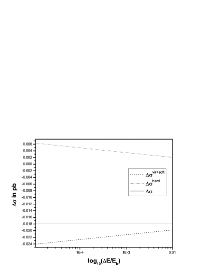
Except above SM and MSSM input parameters, we have to input some other parameters in our numerical calculations, for example, the IR regularization parameter $m_{\gamma}$ and the soft cutoff $\Delta E_{\gamma}/E_{b}$. In our following numerical calculations, we take $\Delta E_{\gamma}/E_{b}=10^{-4}$ and $m_{\gamma}=10^{-5}~{}GeV$, if there is no other statement. As we know, the final results should be independent on the IR regulator $m_{\gamma}$ and the soft cutoff $\Delta E_{\gamma}/E_{b}$. For demonstration, we present the Fig.3, which shows the corrections to the cross section of the subprocess $\gamma\gamma\to H^{+}H^{-}$ versus the soft cutoff $\Delta E_{g}/E_{b}$ in conditions of $M_{H^{\pm}}=250~{}GeV$, $\sqrt{\hat{s}}=1000~{}GeV$ and the input parameters in $Set~{}1$(see below). The dashed, dotted and solid lines correspond to $\Delta\hat{\sigma}_{vir+soft}$, $\Delta\hat{\sigma}_{hard}$ and the total one-loop electroweak correction $\Delta\hat{\sigma}$, respectively. As shown in this figure, the full one-loop EW correction $\Delta\hat{\sigma}$ is independent of the soft cutoff $\Delta E_{\gamma}/E_{b}$ as $\Delta E_{\gamma}/E_{b}$ running from $10^{-5}$ to $10^{-2}$, although both $\Delta\hat{\sigma}_{vir+soft}$ and $\Delta\hat{\sigma}_{hard}$ depend on the soft cutoff strongly.

Figure 3: The full one-loop corrections to the subprocess $\gamma\gamma\to H^{+}H^{-}$ as the functions of the soft cutoff $\Delta E/E_{b}$.

In order to show the numerical results and discuss the effects of the radiative corrections to the subprocess of $\gamma\gamma\to H^{+}H^{-}$ quantitatively, we choose the following four typical input data sets:

• $\tan\beta=4$, $M_{H^{\pm}}=250~{}~{}or~{}~{}500$ GeV, $M_{SUSY}=200$ GeV, $\mu=600$ GeV, $M_{2}=200$ GeV and $A_{f}=400$ GeV.

• $\tan\beta=20$, $M_{H^{\pm}}=250~{}~{}or~{}~{}500$ GeV, $M_{SUSY}=400$ GeV, $\mu=1000$ GeV, $M_{2}=200$ GeV and $A_{f}=800$ GeV.

• $\tan\beta=40$, $M_{H^{\pm}}=250~{}~{}or~{}~{}500$ GeV, $M_{SUSY}=200$ GeV, $\mu=200$ GeV, $M_{2}=1000$ GeV and $A_{f}=300$ GeV.

With the input parameters $\tan\beta$, $M_{H^{\pm}}$, $M_{SUSY}$, $\mu$, $M_{2}$ and $A_{f}$ in one of the above data sets, we can obtain all the masses of supersymmetric particles by using package FormCalc[26]. The input data $Set1$(or $Set2$) with small(or mediate) $\tan\beta$, makes the gaugino-like case with lighter(or heavier) sfermions, while the input data $Set3$ with larger $\tan\beta$ induces higgsino-like case.

We also give the results at the SPS1a’ point from the SPA project[28]. The fundamental SUSY parameters in SPA project are compatible with all available precision data and actual mass and cosmological bounds. The SPA convention parameters are defined in the $\overline{DR}$ scheme at the scale of $Q=1~{}TeV$. A translation from these parameters to our on-mass-shell definition can be performed by subtracting the corresponding counter terms, i.e. ${\cal P}^{\rm OMS}={\cal P}(Q)-\delta{\cal P}(Q)$. Then we get the pole mass of charged Higgs as $M_{H^{\pm}}=438.6GeV$. For all other parameters that do not enter in the tree-level calculations, either $\overline{DR}$ or OMS value can be used, since their difference is of higher order.

Figure 4: The Born and the full one-loop level electroweak corrected cross sections of the subprocess $\gamma\gamma\to H^{+}H^{-}$ versus c.m.s. energy $\sqrt{\hat{s}}$ are plotted in Fig.4(a)($M_{H^{\pm}}=250GeV$) and Fig.4(c)($M_{H^{\pm}}=500GeV$)). The corresponding relative corrections as the functions of the c.m.s energy $\sqrt{\hat{s}}$ are shown in Fig.4(b) and Fig.4(d), respectively.

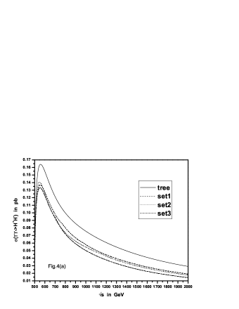
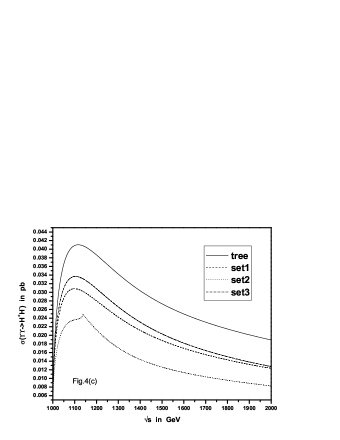
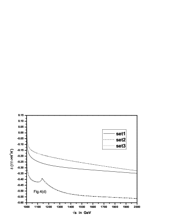
The Born and the full one-loop level electroweak corrected cross sections for the subprocess $\gamma\gamma\to H^{+}H^{-}$ as the functions of c.m.s. energy of $\gamma\gamma$ collision with above three input data sets are displayed in Fig.4(a) with $M_{H^{\pm}}=250~{}GeV$ and in Fig.4(c) with $M_{H^{\pm}}=500~{}GeV$, respectively. The corresponding relative corrections are depicted in Fig.4(b) and Fig.4(d). We can see that when $\sqrt{\hat{s}}\sim 558~{}(1118)$ GeV, the tree level cross section reaches the maximal value 0.164 (0.041) pb in Fig.4(a) (Fig.4(c)). But its maximum value is shifted to 0.141 (0.337) pb after including the one-loop SUSY EW corrections. On the curve for the input data $Set~{}1$ in Fig.4(b) there exist small resonance spikes in the regions around the vicinities of $\sqrt{\hat{s}}\sim 2m_{\tilde{t}_{1}}\sim 762.5~{}GeV$ and $\sqrt{\hat{s}}\sim 2m_{\tilde{t}_{2}}\sim 968.3~{}GeV$. On the curve for input data $Set~{}2$ the resonance peak is located at $\sqrt{\hat{s}}\sim 2m_{\tilde{t}_{2}}\sim 1137.1~{}GeV$. For the curves of the input data $Set~{}3$, the resonance effect can be seen around the position of $\sqrt{\hat{s}}\sim 2m_{\tilde{\tau}_{1}}\sim 715.4~{}GeV$. On the curves for the input data $Set~{}2$ in both Fig.4(c) and Fig.4(d), we can see the resonance spikes at $\sqrt{\hat{s}}\sim 2m_{\tilde{t}_{2}}\sim 1137.1~{}GeV$. Both Fig.4(b) and Fig.4(d) show that the relative corrections have their maximal values at the position near the threshold energies and then decrease quantitatively with the increment of $\sqrt{\hat{s}}$. At the position of colliding energy $\sqrt{\hat{s}}=2~{}TeV$ shown in Fig.4(b) (Fig.4(d)), the relative electroweak correction can reach $-34.5\%~{}(-34.8\%)$, $-39.4\%~{}(-56.4\%)$ and $-60.1\%~{}(-32.6\%)$ for input data $Set~{}1$, $Set~{}2$ and $Set~{}3$, respectively. We can see from Fig.4(b) that the absolute relative corrections for the input data $Set~{}3$ can be rather large, and are generally larger than the corresponding ones for the input data $Set~{}1$ and $Set~{}2$. That is because in the input data $Set~{}3$ we have a very small sbottom mass $m_{\tilde{b}_{1}}=76.67~{}GeV$. While Fig.4(d) shows that the absolute relative corrections for the input data $Set~{}2$ are the largest among all the three input data sets, since there the conditions of $m_{\tilde{l}_{i},\tilde{U}_{i},\tilde{D}_{i}}\sim M_{H^{\pm}}=500~{}GeV(i=1,2)$ are satisfied.

Figure 5: The full one-loop relative electroweak corrections for the subprocess $\gamma\gamma\to H^{+}H^{-}$ as the functions of the charged Higgs mass $M_{H^{\pm}}$.

In Fig.5 we present the full one-loop relative electroweak corrections for the subprocess $\gamma\gamma\to H^{+}H^{-}$ as the functions of the charged Higgs mass $M_{H^{\pm}}$ with input data $Set~{}1$, $Set~{}2$ and $Set~{}3$ separately. The corresponding collision energies in the c.m.s. of incoming $\gamma\gamma$, $\sqrt{\hat{s}}$, are $1000~{}GeV$, $1500~{}GeV$ and $2000~{}GeV$, respectively. As shown in the figure all the curves are less sensitive to $M_{H^{\pm}}$, except in the region of $M_{H^{\pm}}>390~{}GeV$. For the curve with the input data $Set~{}3$, the resonance effect can be seen around the positions of $M_{H^{\pm}}\sim m_{\tilde{t}_{1}}+m_{\tilde{b}_{2}}\sim 410.6~{}GeV$ and $M_{H^{\pm}}\sim m_{\tilde{t}_{2}}+m_{\tilde{b}_{1}}\sim 426.2~{}GeV$. In this figure the curve for the input data $Set~{}1$ shows that the relative correction is almost stable except in the energy region approaching the threshold $\sqrt{\hat{s}}\sim 2M_{H^{\pm}}\sim 1000~{}GeV$. However, the curve for the input data set $Set~{}3$ varies sharply in the region of $380~{}GeV<M_{H^{\pm}}<440~{}GeV$ due to the resonance effects.

Figure 6: The full one-loop relative electroweak corrections for the subprocess $\gamma\gamma\to H^{+}H^{-}$ as the functions of $\tan\beta$.

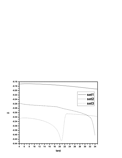
In each figure of Fig.6, Fig.7 and Fig.8, we take the input parameter sets as: $Set~{}1$, $Set~{}2$ and $Set~{}3$, except the charge Higgs mass being $200~{}GeV$, $300~{}GeV$ and $500~{}GeV$, the colliding energy being $500~{}GeV$, $1000~{}GeV$ and $2000~{}GeV$, respectively. In Fig.6 we present the full one-loop relative electroweak corrections for the subprocess $\gamma\gamma\to H^{+}H^{-}$ as the functions of the ratio of the vacuum expectation values $\tan\beta$. We can see from the curves for input data $Set~{}1$ and $Set~{}2$ that the relative corrections decrease slowly with the increment of $\tan\beta$ except the curve for $Set~{}2$ in the region of $\tan\beta>32$. For the curve of the input data $Set~{}3$, the resonance effect can be seen around the position of $\tan\beta\sim 21$ where the condition of $M_{H^{\pm}}\sim m_{\tilde{t}_{2}}+m_{\tilde{b}_{1}}\sim 500~{}GeV$ is satisfied.

Figure 7: The full one-loop relative electroweak corrections for the subprocess $\gamma\gamma\to H^{+}H^{-}$ as the functions of $M_{SUSY}$.

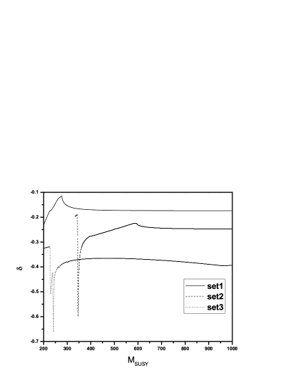
In Fig.7 we present the full one-loop relative electroweak corrections for the subprocess $\gamma\gamma\to H^{+}H^{-}$ as the functions of $M_{SUSY}$. We can see that the relative corrections are not sensitive to $M_{SUSY}$ except at the vicinities of the resonance points. For the curve of the input data $Set~{}1$, the resonance effect can be seen around the position of $M_{SUSY}\sim 276~{}GeV$ where $\sqrt{\hat{s}}\sim 2m_{\tilde{t}_{1}}\sim 500~{}GeV$. For the curve of the input data $Set~{}2$, the resonance effect can be seen around the positions of $M_{SUSY}\sim 346$ GeV (where $M_{H^{\pm}}\sim m_{\tilde{t}_{1}}+m_{\tilde{b}_{1}}\sim 300~{}GeV$) and $M_{SUSY}\sim 594~{}GeV$ (where $\sqrt{\hat{s}}\sim 2m_{\tilde{t}_{1}}\sim 1000~{}GeV$). For the curve of the input data $Set~{}3$, the resonance effect can be seen around the positions of $M_{SUSY}\sim 230~{}GeV$ (where $M_{H^{\pm}}\sim m_{\tilde{t}_{2}}+m_{\tilde{b}_{1}}\sim 500~{}GeV$) and $M_{SUSY}\sim 242~{}GeV$ (where $M_{H^{\pm}}\sim m_{\tilde{t}_{1}}+m_{\tilde{b}_{2}}\sim 500~{}GeV$).

Figure 8: The full one-loop relative electroweak corrections for the subprocess $\gamma\gamma\to H^{+}H^{-}$ as the functions of $M_{2}$.

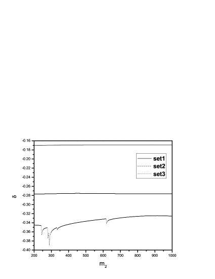
In Fig.8 we present the full one-loop relative electroweak corrections to the subprocess $\gamma\gamma\to H^{+}H^{-}$ as the functions of $M_{2}$. We can see that the relative corrections are not sensitive to $M_{2}$ except the curve for the input data $Set~{}3$. On the curve of the input data $Set~{}3$, there are five resonance points which come from the fact that the masses of some chargino and neutralino are lighter than $M_{H^{\pm}}$. The resonance effect can be seen around the positions of $M_{2}\sim 244$ GeV (where $M_{H^{\pm}}\sim m_{\tilde{\chi}^{+}_{2}}+m_{\tilde{\chi}^{0}_{3}}\sim 500~{}GeV$), $M_{2}\sim 280$ GeV (where $M_{H^{\pm}}\sim m_{\tilde{\chi}^{+}_{2}}+m_{\tilde{\chi}^{0}_{2}}\sim 500~{}GeV$), $M_{2}\sim 288$ GeV (where $M_{H^{\pm}}\sim m_{\tilde{\chi}^{+}_{1}}+m_{\tilde{\chi}^{0}_{4}}\sim 500~{}GeV$), $M_{2}\sim 334$ GeV (where $M_{H^{\pm}}\sim m_{\tilde{\chi}^{+}_{2}}+m_{\tilde{\chi}^{0}_{1}}\sim 500~{}GeV$) and $M_{2}\sim 620$ GeV (where $M_{H^{\pm}}\sim m_{\tilde{\chi}^{+}_{1}}+m_{\tilde{\chi}^{0}_{3}}\sim 500~{}GeV$). For the input data set $Set~{}1$ and $Set~{}2$, the relative corrections are almost stable, the relative corrections are about $-16.9\%$ and $-27.6\%$, respectively.

Figure 9: The Born and the full one-loop level electroweak corrected cross sections for the parent process $e^{+}e^{-}\to\gamma\gamma\to H^{+}H^{-}$, are shown in Fig.9(a)($M_{H^{\pm}}=250GeV$) and Fig.9(c)($M_{H^{\pm}}=500GeV$), respectively. The corresponding relative corrections as the functions of the c.m.s energy of the incoming electron-positron pair, are shown in Fig.9(b) and Fig.9(d), separately.

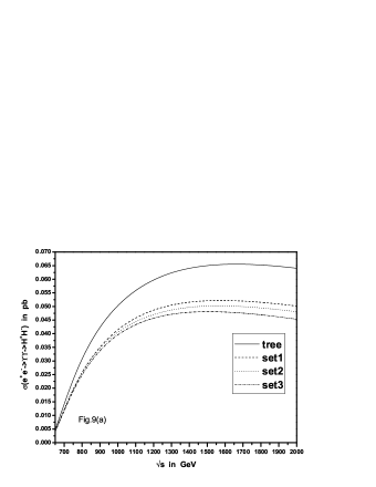
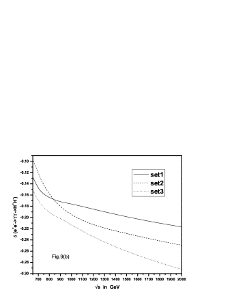
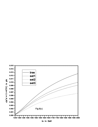
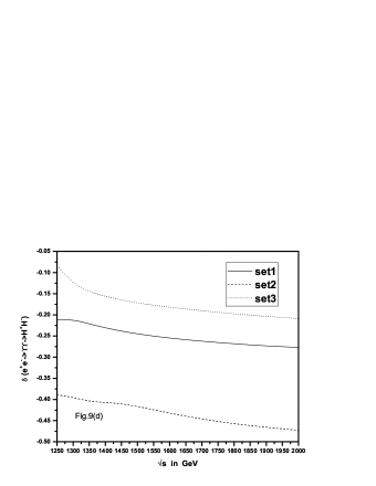
Fig.9(a) is the plot of the Born and the full one-loop level electroweak corrected cross sections for the parent process $e^{+}e^{-}\to\gamma\gamma\to H^{+}H^{-}$ versus the electron-positron colliding energy with $M_{H^{\pm}}=250GeV$. At the position of $\sqrt{s}\sim 1.5~{}TeV$ the cross sections reach their maximal values, e.g., for the curve of the input data $Set~{}1$, the cross section has the maximal value $52.2~{}fb$. When $\sqrt{s}>1.5~{}TeV$, the cross sections decrease slowly with the increment of the colliding $e^{+}e^{-}$ c.m.s energy. Fig.9(b) shows the corresponding relative corrections as the functions of colliding $e^{+}e^{-}$ energy. We can see that the absolute relative corrections increase obviously with the increment of $\sqrt{s}$. When $\sqrt{\hat{s}}=2~{}TeV$, the relative correction can reach its maximal value $-29.2\%$ for the curve of the input data $Set~{}3$. Fig.9(c) is the plot of the Born and the full one-loop level electroweak corrected cross sections for the parent process $e^{+}e^{-}\to\gamma\gamma\to H^{+}H^{-}$ versus the electron-positron colliding energy with $M_{H^{\pm}}=500GeV$. The cross sections increase with the increment of the colliding c.m.s energy. When $\sqrt{s}=2~{}TeV$, the corrected cross section reaches its maximal value $10.9~{}fb$ for the input data $Set~{}3$. Fig.9(d) shows the corresponding relative corrections as the functions of the colliding $e^{+}e^{-}$ energy. We can see that the absolute relative corrections increase apparently with the increment of $\sqrt{s}$. When $\sqrt{s}=2~{}TeV$, the relative correction can reach $-47.3\%$ for the input data $Set~{}3$.

Figure 10: The Born and the full one-loop level electroweak corrected cross sections for the subprocess $\gamma\gamma\to H^{+}H^{-}$(parent process $e^{+}e^{-}\to\gamma\gamma\to H^{+}H^{-}$), and their corresponding relative corrections as the functions of the c.m.s colliding energy $\sqrt{\hat{s}}(\sqrt{s})$ at the SPS1a’ point are shown in Fig.10(a) and Fig.10(b)(Fig.10(c) and Fig.10(d)), respectively.

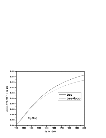
Fig.10(a) and Fig.10(b) shows the Born and the full one-loop level electroweak corrected cross sections and the corresponding relative corrections for the subprocess $\gamma\gamma\to H^{+}H^{-}$ as the functions of the c.m.s energy $\sqrt{\hat{s}}$ at the SPS1a’ point. From Fig.10(a) we can see that the cross sections decrease with the increment of the colliding c.m.s energy $\sqrt{\hat{s}}$ when $\sqrt{\hat{s}}>1~{}TeV$. At the point of $\sqrt{\hat{s}}=980~{}GeV$, the tree level and one-loop level corrected cross sections are $53.2~{}fb$ and $49.4~{}fb$, respectively. When $\sqrt{\hat{s}}=2~{}TeV$, the tree level and one-loop level corrected cross sections go down to $21.0~{}fb$ and $15.7~{}fb$, respectively. In Fig.10(b) we can see that there are two small peaks at the vicinities of $\sqrt{\hat{s}}\sim 2m_{\tilde{c}_{2}}\sim 1048.3~{}GeV$ and $\sqrt{\hat{s}}\sim 2m_{\tilde{t}_{2}}\sim 1137.4~{}GeV$. The absolute relative correction increases with the increment of $\sqrt{\hat{s}}$. When $\sqrt{\hat{s}}$ goes from $1~{}TeV$ to $2~{}TeV$, the relative correction varies from $-7.76\%$ to $-19.5\%$. Fig.10(c) and Fig.10(d) are the plots for the cross sections and the corresponding relative corrections of the parent process $e^{+}e^{-}\to\gamma\gamma\to H^{+}H^{-}$ as the functions of the c.m.s energy of the incoming electron-positron pair, separately. From Fig.10(c) we can see that the cross sections increase with the increment of the colliding $e^{+}e^{-}$ c.m.s energy $\sqrt{s}$. When $\sqrt{s}=2~{}TeV$, the tree level and one-loop level corrected cross sections are $18.7~{}fb$ and $16.8~{}fb$, respectively. In Fig.10(d) we can see that the absolute relative correction increases with the increment of $\sqrt{s}$. When $\sqrt{s}$ goes from $1.1~{}TeV$ to $2~{}TeV$, the relative correction varies from $-0.86\%$ to $-10.2\%$.

V Summary

In this paper, we present the calculation of the full one-loop electroweak corrections to the subprocess $\gamma\gamma\to H^{+}H^{-}$ and parent process $e^{+}e^{-}\to\gamma\gamma\to H^{+}H^{-}$ at a linear collider in the MSSM. We analyze the dependence of the relative corrections for the subprocess on colliding energy, charged Higgs boson mass and several supersymmetric parameters. We find that these corrections generally reduce the Born cross sections and the relative corrections are typically few dozen percent for both the subprocess and the parent process . With the input data $Set~{}3$, the relative corrections to the subprocess are obviously sensitive to $M_{H^{\pm}}$, $\tan\beta$, $M_{SUSY}$ and $M_{2}$ in some parameter space due to the resonance effects. However, with the input data $Set~{}1$ and $Set~{}2$, the relative corrections to the subprocess are less sensitive to these parameters comparing with the curves with input data $Set~{}3$. We also give the numerical results at the SPS1a’ point, it shows that with $\sqrt{\hat{s}}$ varying from $1~{}TeV$ to $2~{}TeV$, the relative correction to the subprocess runs from $-7.76\%$ to $-19.5\%$. We conclude that the complete one-loop electroweak corrections to both subprocess $\gamma\gamma\to H^{+}H^{-}$ and the parent process $e^{+}e^{-}\to\gamma\gamma\to H^{+}H^{-}$ are generally significant and should be considered in the precise analysis.

Acknowledgments: This work was supported in part by the National Natural Science Foundation of China and and a special fund sponsored by China Academy of Science.

Figure Captions

Figure 1 The leading order diagrams for the $\gamma\gamma\to H^{+}H^{-}$ subprocess.

Figure 2 The real photon emission diagrams for the subprocess $\gamma\gamma\to H^{+}H^{-}\gamma$.

Figure 3 The full one-loop corrections to the subprocess $\gamma\gamma\to H^{+}H^{-}$ as the functions of the soft cutoff $\Delta E/E_{b}$.

Figure 4 The Born and the full one-loop level electroweak corrected cross sections of the subprocess $\gamma\gamma\to H^{+}H^{-}$ versus c.m.s. energy $\sqrt{\hat{s}}$ are plotted in Fig.4(a)($M_{H^{\pm}}=250GeV$) and Fig.4(c)($M_{H^{\pm}}=500GeV$)). The corresponding relative corrections as the functions of the c.m.s energy $\sqrt{\hat{s}}$ are shown in Fig.4(b) and Fig.4(d), respectively.

Figure 5 The full one-loop relative electroweak corrections for the subprocess $\gamma\gamma\to H^{+}H^{-}$ as the functions of the charged Higgs mass $M_{H^{\pm}}$.

Figure 6 The full one-loop relative electroweak corrections for the subprocess $\gamma\gamma\to H^{+}H^{-}$ as the functions of $\tan\beta$.

Figure 7 The full one-loop relative electroweak corrections for the subprocess $\gamma\gamma\to H^{+}H^{-}$ as the functions of $M_{SUSY}$.

Figure 8 The full one-loop relative electroweak corrections for the subprocess $\gamma\gamma\to H^{+}H^{-}$ as the functions of $M_{2}$.

Figure 9 The Born and the full one-loop level electroweak corrected cross sections for the parent process $e^{+}e^{-}\to\gamma\gamma\to H^{+}H^{-}$, are shown in Fig.9(a)($M_{H^{\pm}}=250GeV$) and Fig.9(c)($M_{H^{\pm}}=500GeV$), respectively. The corresponding relative corrections as the functions of the c.m.s energy of the incoming electron-positron pair, are shown in Fig.9(b) and Fig.9(d), separately.

Figure 10 The Born and the full one-loop level electroweak corrected cross sections for the subprocess $\gamma\gamma\to H^{+}H^{-}$(parent process $e^{+}e^{-}\to\gamma\gamma\to H^{+}H^{-}$), and their corresponding relative corrections as the functions of the c.m.s colliding energy $\sqrt{\hat{s}}(\sqrt{s})$ at the SPS1a’ point are shown in Fig.10(a) and Fig.10(b)(Fig.10(c) and Fig.10(d)), respectively.

References

- [1] H. E. Haber and G. L. Kane, Phys. Rep. 117 (1985) 75.
- [2] C. Adolphsen et al. (International Study Group Collaboration), ”International study group progress report on linear collider development,” SLAC-R-559 and KEK-REPORT-2000-7 (April, 2000).
- [3] N. Akasaka et al., ”JLC design study,” KEK-REPORT-97-1
- [4] R. Brinkmann, K. Flottmann, J. Rossbach, P. Schmuser, N. Walker and H. Weise(editor), ”TESLA: The superconducting electron positron linear collider with an integrated X-ray laser laboratory. Technical design report, Part 2: The Accelerator,” DESY-01-11 (March, 2001).
- [5] ”A 3TeV Linear Collider Based on CLIC Technology”, G.Guignard(editor), CERN-2000-008.
- [6] Yi Jiang, Wen-Gan Ma, Liang Han, Meng Han and Zeng-Hui Yu, J. Phys. G24, 83(1998); S.S.D. Willenbrock, Phys. Rev. D 35, 173 (1987); Yi Jiang, Wen-Gan Ma, Liang Han, Meng Han and Zeng-Hui Yu, J. Phys. G 23, 385 (1997), Erratum, ibidem G 23, 1151 (1997); A. Krause, T. Plehn, M. Spira and P.M. Zerwas, Nucl. Phys. B 519, 85 (1998); A. Belyaev, M. Drees, O.J.P. Eboli, J.K. Mizukoshi and S.F. Novaes, Phys. Rev. D60, 075008 (1999); A. Belyaev, M. Drees and J.K. Mizukoshi, Eur. Phys. J. C 17, 337 (2000); O. Brein and W. Hollik, Eur. Phys. J. C 13, 175(2000).
- [7] Hong-Sheng Hou, Wen-Gan Ma, Ren-You Zhang, Yi Jiang, Liang Han, Li-Rong Xing, Phys. Rev.D71, 075014 (2005); A.A. Barrientos Bendezú and B.A. Kniehl, Nucl. Phys. B 568, 305 (2000); S. Moretti, J. Phys. G 28, 2567 (2002).
- [8] A. Arhrib, M.C. Peyranere, and G. Moultaka, Phys.Lett.B341,313(1995).
- [9] Jaume Guasch, Wolfgang Hollik, and Arnd Kraft, hep-ph/9911452.
- [10] Wen-Gan Ma, C. S. Li, and Liang Han, Phys. Rev. D53, 1304 (1996).
- [11] Shou Hua Zhu, Chong Sheng Li, and Chong Shou Gao, Phys.Rev. D58 (1998) 055007.
- [12] I.F. Ginzburg, G.L. Kotkin, V.G. Serbo and V.I. Telov, Nucl. Instrum. Meth. Nucl. Instrum. Meth. A205, 47(1983); I.F. Ginzburg, G.L. Kotkin, V.G. Panfil, V.G. Serbo and V.I. Telov, Nucl. Instrum. Meth. A219, 5(1984);
- [13] Bernd A. Kniehl, Phys. Rep. 240(1994)211.
- [14] D. M. Copper, D. R. T. Jones, and P. van Nieuwenhuizen, Nucl. Phys. B167, 479 (1980); W. Siegel, Phys. Lett. 84B, 193 (1979)
- [15] D. A. Ross and J. C. Taylor, Nucl. Phys. B51, 25 (1979).
- [16] T. Hahn, Comp. Phys. Commun. 140, 418(2001).
- [17] C. Weber, H. Eberl, W. Majerotto, Phys. Lett. B572(2003) 56, hep-ph/0305250.
- [18] H. Eberl, M. Kincel, W. Majerotto and Y. Yamada, Nucl. Phys. B625(2002) 372, hep-ph/0111303.
- [19] K. Kovařík, C. Weber, H. Eberl, W. Majerotto, Phys.Lett. B591 (2004) 242-254.
- [20] W.T. Giele and E.W.N. Glover, Phys. Rev. D46, 1980 (1992); W.T. Giele, E.W. Glover and D.A. Kosower, Nucl. Phys. B403, 633 (1993); S. Keller and E. Laenen, Phys. Rev. D59, 114004 (1999).
- [21] A. Denner, Fortschr. Phys. 41, 307 (1993).
- [22] G.’t Hooft and M. Veltman, Nucl. Phys. B153, 365 (1979).
- [23] V. Telnov, Nucl. Instrum. Methods Phys. Res. A294(1990)72; L. Ginzburg, G. Kotkin and H. Spiesbergerm, Fortschr. Phys. 34(1986)687.
- [24] Particle Data Group, Eur. Phys. J. C15 2000.
- [25] F. Jegerlehner, DESY 01-029, hep-ph/0105283.
- [26] Thomas Hahn and Christian Schappacher,Comput.Phys.Commun. 143(2002)54-68, hep-ph/0105349.
- [27] J. F. Gunion, H. E. Haber, Nucl. Phys. B272 (1986) 1.
- [28] SPA project, http://spa.desy.de/spa/
- [29] W. Oeller, H. Eberl, and W. Majerotto, Phys.Rev. D71 (2005) 115002.