Pole wave-function renormalization prescription for unstable particles

Abstract

We base a new wave-function renormalization prescription on the pole mass renormalization prescription, in which the Wave-function Renormalization Constant (WRC) is extracted by expanding the particle’s propagator around its pole, rather than its physical mass point as convention. We find the difference between the new and the conventional WRC is gauge-parameter dependent for unstable particles beyond one-loop level, which will lead to some physical results gauge dependent under the conventional wave-function renormalization prescription beyond one-loop level.

I Introduction

The conventional wave-function renormalization prescription extracts WRC by expanding the particle’s propagator around its physical mass point in the LSZ reduction formula c1 . For scalar boson it is c2 ; c3 ; c5

$$\frac{i}{p^{2}-m^{2}-\delta m^{2}+\Sigma(p^{2})} \sim \frac{i}{(p^{2}-m^{2})(1+Re\Sigma^{\prime}(m^{2}))+Re\Sigma(m^{2})-\delta m^{2}+i\,Im\Sigma(p^{2})}$$

$$= \frac{i\,(1+Re\Sigma^{\prime}(m^{2}))^{-1}}{p^{2}-m^{2}+i\,\epsilon}\,,$$

$${\bf or}\hskip 8.53581pt \sim \frac{i}{(p^{2}-m^{2})(1+\Sigma^{\prime}(m^{2}))+\Sigma(m^{2})-\delta m^{2}}\,=\,\frac{i\,(1+\Sigma^{\prime}(m^{2}))^{-1}}{p^{2}-m^{2}+i\,\epsilon^{\prime}}\,,$$ (1)

where $\Sigma^{\prime}(m^{2})=\partial\Sigma(m^{2})/\partial p^{2}$, $\epsilon$ and $\epsilon^{\prime}$ are small quantities. But not long ago people propose that only the mass definition of the pole of the particle’s propagator is gauge invariant c6 and physical results are only gauge invariant under the pole mass renormalization prescription c9 , so WRC must also be defined on the pole of the particle’s propagator. Considering the fact that unstable particle’s WRC must contain imaginary part c3 ; c5 ; cin ; c4 , the new wave-function renormalization prescription for boson must be

$$\frac{i}{p^{2}-m^{2}-\delta m^{2}+\Sigma(p^{2})}\,\sim\,\frac{i}{(p^{2}-\bar{s})(1+\Sigma^{\prime}(\bar{s}))}\,=\,\frac{i\,(1+\Sigma^{\prime}(\bar{s}))^{-1}}{p^{2}-\bar{s}}\,,$$ (2)

where $\bar{s}=m^{2}-im\Gamma$ is the pole of the boson’s propagator c6 . Note that the pole mass renormalization prescription has been used in Eq.(2).

For fermion the new wave-function renormalization prescription is a little complex. The fermion inverse propagator can be written as

$$iS^{-1}({\hbox to0.0pt{$p$\hss}/})\,=\,{\hbox to0.0pt{$p$\hss}/}-m-\delta m+\Sigma({\hbox to0.0pt{$p$\hss}/})\,\equiv\,{\hbox to0.0pt{$p$\hss}/}(a\gamma_{L}+b\gamma_{R})+c\gamma_{L}+d\gamma_{R}\,,$$ (3)

where $\gamma_{L}$ and $\gamma_{R}$ are the left- and right- handed helicity operators, and the diagonal fermion self energy is

$$\Sigma({\hbox to0.0pt{$p$\hss}/})\,=\,{\hbox to0.0pt{$p$\hss}/}\gamma_{L}\,\Sigma^{L}(p^{2})+{\hbox to0.0pt{$p$\hss}/}\gamma_{R}\,\Sigma^{R}(p^{2})+m(\gamma_{L}\Sigma^{S,L}(p^{2})+\gamma_{R}\Sigma^{S,R}(p^{2}))\,.$$ (4)

Expanding the fermion propagator around its pole we get cin ; c4

$$S({\hbox to0.0pt{$p$\hss}/}) = \frac{i({\hbox to0.0pt{$p$\hss}/}(a\gamma_{L}+b\gamma_{R})-d\gamma_{L}-c\gamma_{R})}{p^{2}ab-cd}$$ (5)

$$\sim \frac{i(m+\delta m+{\hbox to0.0pt{$p$\hss}/}\gamma_{L}(1+\Sigma^{L}(\bar{s}))+{\hbox to0.0pt{$p$\hss}/}\gamma_{R}(1+\Sigma^{R}(\bar{s}))-m\gamma_{L}\Sigma^{S,R}(\bar{s})-m\gamma_{R}\Sigma^{S,L}(\bar{s}))}{(p^{2}-m^{2}+i\,m\,\Gamma)A}\,,$$

where $\bar{s}=m^{2}-im\Gamma$ is the pole of the fermion propagator, and

$$A = (1+\Sigma^{L}(\bar{s}))(1+\Sigma^{R}(\bar{s}))+\bar{s}(\Sigma^{L\prime}(\bar{s})+\Sigma^{R\prime}(\bar{s})+\Sigma^{L\prime}(\bar{s})\Sigma^{R}(\bar{s})+\Sigma^{L}(\bar{s})\Sigma^{R\prime}(\bar{s}))$$ (6)

$$+ m\Sigma^{S,L\prime}(\bar{s})(m+\delta m-m\Sigma^{S,R}(\bar{s}))+m\Sigma^{S,R\prime}(\bar{s})(m+\delta m-m\Sigma^{S,L}(\bar{s}))\,.$$

From Eq.(2) and Eq.(5) we can extract boson and fermion’s WRC. In section 2 we will do this work. In section 3 we will evaluate the difference of unstable particle’s WRC between the new and the conventional wave-function renormalization prescription and discuss the influence of the difference on physical results. Lastly we give our conclusion.

II Determination of wave-function renormalization constants

In the LSZ reduction formula one needs to introduce two sets of WRC: the incoming WRC and the outgoing WRC c5 ; cin ; c4 . For boson the incoming and outgoing WRC are introduced as follows c5

$$Z^{\frac{1}{2}}\,=\,<\Omega|\phi(0)|\lambda>\,,\hskip 28.45274pt\bar{Z}^{\frac{1}{2}}\,=\,<\lambda|\phi^{\dagger}(0)|\Omega>\,,$$ (7)

where $\Omega$ is the interaction vacuum, $\phi$ is the boson’s Heisenberg field, and $\lambda$ is the incoming or outgoing state of S-matrix element. According to the LSZ reduction formula we have from Eq.(2)

$$Z^{\frac{1}{2}}\bar{Z}^{\frac{1}{2}}\,=\,(1+\Sigma^{\prime}(m^{2}-i\,m\,\Gamma))^{-1}\,.$$ (8)

Another condition that boson’s WRC must satisfy is c5

$$\bar{Z}\,=\,Z\,.$$ (9)

Therefore we get

$$\bar{Z}\,=\,Z\,=\,(1+\Sigma^{\prime}(m^{2}-i\,m\,\Gamma))^{-1}\,.$$ (10)

For fermion the incoming and outgoing WRC are introduced as follows c5 :

$$<\Omega|\psi(0)|\lambda>\,=\,Z^{\frac{1}{2}}u\,,\hskip 28.45274pt<\lambda|\bar{\psi}(0)|\Omega>\,=\,\bar{u}\bar{Z}^{\frac{1}{2}}\,,$$ (11)

where $\psi$ is the fermion’s Heisenberg field and

$$Z^{\frac{1}{2}}\,=\,Z^{L\frac{1}{2}}\gamma_{L}+Z^{R\frac{1}{2}}\gamma_{R}\,,\hskip 28.45274pt\bar{Z}^{\frac{1}{2}}\,=\,\bar{Z}^{L\frac{1}{2}}\gamma_{R}+\bar{Z}^{R\frac{1}{2}}\gamma_{L}\,.$$ (12)

The fermion propagator at resonant region can be expressed as c5 ; cin

$$S({\hbox to0.0pt{$p$\hss}/})\,\sim\,\frac{i\,Z^{\frac{1}{2}}({\hbox to0.0pt{$p$\hss}/}+m+ix)\bar{Z}^{\frac{1}{2}}}{p^{2}-m^{2}+i\,m\,\Gamma}\,,$$ (13)

where $x$ is a small quantity. Considering Eqs.(5,13) must be placed in the middle of on-shell spinors $\bar{u}$ and $u$ (or $\bar{\nu}$ and $\nu$) and the fact $\bar{u}\gamma_{L}u=\bar{u}\gamma_{R}u$ (or $\bar{\nu}\gamma_{L}\nu=\bar{\nu}\gamma_{R}\nu$), we obtain

$$Z^{L\frac{1}{2}}\bar{Z}^{L\frac{1}{2}} = (1+\Sigma^{R}(\bar{s}))/A\,,$$

$$Z^{R\frac{1}{2}}\bar{Z}^{R\frac{1}{2}} = (1+\Sigma^{L}(\bar{s}))/A\,,$$

$$Z^{L\frac{1}{2}}\bar{Z}^{R\frac{1}{2}}+Z^{R\frac{1}{2}}\bar{Z}^{L\frac{1}{2}} = (2m+2\delta m-m\Sigma^{S,L}(\bar{s})-m\Sigma^{S,R}(\bar{s}))/(A(m+i\,x))\,.$$ (14)

Another condition that fermion’s WRC must satisfy is c5

$$\bar{Z}^{L}\,=\,Z^{L}\,,\hskip 28.45274pt\bar{Z}^{R}\,=\,Z^{R}\,.$$ (15)

Therefore we get

$$\bar{Z}^{L} = Z^{L}\,=\,(1+\Sigma^{R}(\bar{s}))/A\,,$$

$$\bar{Z}^{R} = Z^{R}\,=\,(1+\Sigma^{L}(\bar{s}))/A\,.$$ (16)

Since the quantity $x$ is undefined in Eq.(13), the third equation of Eqs.(14) can be used to define $x$. At one-loop level we get cin

$$x\,=\,-\Gamma/2$$ (17)

where $\Gamma$ is the fermion’s decay width.

Now we have finished the definition of diagonal WRC. The off-diagonal WRC are out of our consideration, because they are different from the diagonal WRC under the meaning of the LSZ reduction formula.

III Gauge dependence of physical results under the conventional wave-function renormalization prescription

Since unstable particle’s WRC must contain imaginary part c3 ; c5 ; cin ; c4 , the conventional wave-function renormalization prescription must be the second prescription of Eq.(1) for boson, i.e. c5 (see Eq.(9))

$$\bar{Z}_{o}\,=\,Z_{o}\,=\,(1+\Sigma^{\prime}(m^{2}))^{-1}\,,$$ (18)

where the subscript $o$ represents the conventional wave-function renormalization prescription. Comparing with Eqs.(10) we find at two-loop level

$$Z_{o}-Z\,=\,-i\,m\,\Gamma\,\Sigma^{\prime\prime}(m^{2})\,.$$ (19)

For unstable boson the difference is gauge-parameter dependent. For example for gauge boson W we obtain (see Fig.1)

$$Re[Z_{oW}-Z_{W}]_{\xi_{W}}$$

$$= \frac{\alpha^{2}}{288s_{w}^{2}}\bigl{[}\sum_{i=e,\mu,\tau}(1-x_{i})^{2}(2+x_{i})+3\sum_{i=u,c}\sum_{j=d,s,b}|V_{ij}|^{2}\sqrt{1-2(x_{i}+x_{j})+(x_{i}-x_{j})^{2}}$$

$$\times (2-(x_{i}+x_{j})-(x_{i}-x_{j})^{2})\bigr{]}(2\xi_{W}^{3}-3\xi_{W}^{2}-6\xi_{W}-5)\theta[1-\xi_{W}]\,,$$ (20)

where $Re$ takes the real part of the quantity, $\xi_{W}$ is the gauge parameter of W, the subscript $\xi_{W}$ denotes the $\xi_{W}$-dependent part of the quantity, $\alpha$ is the fine structure constant, $s_{w}$ is the sine of the weak mixing angle, $x_{i}=m_{i}^{2}/m_{W}^{2}$ and $x_{j}=m_{j}^{2}/m_{W}^{2}$ with $m_{W}$ the mass of W, $V_{ij}$ is the CKM matrix element c11 , and $\theta$ is the Heaviside function. Note that in the calculations we have used the program packages FeynArts and FeynCalc c10 .

Figure 1: W one-loop self-energy diagrams containing imaginary part.

For fermion the conventional wave-function renormalization prescription must be c5

$$\bar{Z}_{o}^{L} = Z_{o}^{L}\,=\,(1+\Sigma^{R}(m^{2}))/A_{1}\,,$$

$$\bar{Z}_{o}^{R} = Z_{o}^{R}\,=\,(1+\Sigma^{L}(m^{2}))/A_{1}\,,$$ (21)

where

$$A_{1} = (1+\Sigma^{L}(m^{2}))(1+\Sigma^{R}(m^{2}))$$ (22)

$$+ m^{2}(\Sigma^{L\prime}(m^{2})+\Sigma^{R\prime}(m^{2})+\Sigma^{L\prime}(m^{2})\Sigma^{R}(m^{2})+\Sigma^{L}(m^{2})\Sigma^{R\prime}(m^{2}))$$

$$+ m\Sigma^{S,L\prime}(m^{2})(m+\delta m-m\Sigma^{S,R}(m^{2}))$$

$$+ m\Sigma^{S,R\prime}(m^{2})(m+\delta m-m\Sigma^{S,L}(m^{2}))\,.$$

Comparing with Eqs.(16) we find

$$Z_{o}^{L}-Z^{L} = -i\,m\,\Gamma(2\Sigma^{L\prime}+\Sigma^{R\prime}+m^{2}(\Sigma^{L\prime\prime}+\Sigma^{R\prime\prime}+\Sigma^{S,L\prime\prime}+\Sigma^{S,R\prime\prime}))\,,$$

$$Z_{o}^{R}-Z^{R} = -i\,m\,\Gamma(\Sigma^{L\prime}+2\Sigma^{R\prime}+m^{2}(\Sigma^{L\prime\prime}+\Sigma^{R\prime\prime}+\Sigma^{S,L\prime\prime}+\Sigma^{S,R\prime\prime}))\,.$$ (23)

For unstable fermion the difference is also gauge-parameter dependent. For example for top quark we obtain (see Fig.2)

$$Re[Z_{ot}^{L}-Z_{t}^{L}]_{\xi_{W}}$$

$$= -\frac{\alpha^{2}}{128s_{w}^{4}x_{t}^{3}}\sum_{i=d,s,b}|V_{ti}|^{2}B_{i}(x_{t}^{2}+(1-2x_{i})x_{t}+x_{i}^{2}+x_{i}-2)$$

$$\times \sum_{j=d,s,b}\frac{|V_{tj}|^{2}}{C_{j}}(x_{t}^{3}-x_{j}x_{t}^{2}-(3\xi_{W}^{2}+3x_{j}\xi_{W}+2x_{j}^{2})x_{t}$$

$$+ 2(\xi_{W}-x_{j})^{2}(\xi_{W}+x_{j}))\theta[m_{t}-\sqrt{\xi_{W}}m_{W}-m_{j}]\,,$$

$$Re[Z_{ot}^{R}-Z_{t}^{R}]_{\xi_{W}}$$

$$= -\frac{\alpha^{2}}{256s_{w}^{4}x_{t}^{3}}\sum_{i=d,s,b}|V_{ti}|^{2}B_{i}(x_{t}^{2}+(1-2x_{i})x_{t}+x_{i}^{2}+x_{i}-2)$$

$$\times \sum_{j=d,s,b}\frac{|V_{tj}|^{2}}{C_{j}}(x_{t}^{3}-(\xi_{W}+x_{j})x_{t}^{2}-(\xi_{W}^{2}+4x_{j}\xi_{W}+3x_{j}^{2})x_{t}$$

$$+ (\xi_{W}-x_{j})^{2}(\xi_{W}+3x_{j}))\theta[m_{t}-\sqrt{\xi_{W}}m_{W}-m_{j}]\,,$$ (24)

where $m_{t}$ is the top quark’s mass and $x_{t}=m_{t}^{2}/m_{W}^{2}$, and

$$B_{i}\,=\,\sqrt{x_{t}^{2}-2(x_{i}+1)x_{t}+(x_{i}-1)^{2}}\,,\hskip 28.45274ptC_{j}\,=\,\sqrt{x_{t}^{2}-2(\xi_{W}+x_{j})x_{t}+(\xi_{W}-x_{j})^{2}}\,.$$ (25)

Figure 2: Top quark’s one-loop self-energy diagrams containing imaginary part.

The gauge dependence of Eqs.(20,24) will lead to the decay widths of some physical processes gauge-parameter dependent under the conventional wave-function renormalization prescription. Considering the physical process $W^{+}\rightarrow e^{+}\nu_{e}$, since positive electron and electronic neutrino are stable particles, their’s WRC are same under the new and the conventional wave-function renormalization prescription, therefore we only need to consider the effect of $Z_{oW}$ on the gauge dependence of the decay width. The result is shown in Fig.3 (the data is cited from Ref.c12 ).

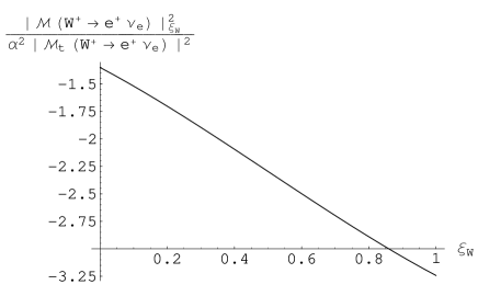
Figure 3: Gauge dependence of two-loop $|\cal{M}$$(W^{+}\rightarrow e^{+}\nu_{e})|^{2}$ under the conventional wave-function renormalization prescription, where $\cal{M}$${}_{t}(W^{+}\rightarrow e^{+}\nu_{e})$ is the tree-level amplitude.

Considering another physical process $t\rightarrow W^{+}b$, since the decay width of bottom quark is zero at one-loop level, the bottom quark’s WRC are same at two-loop level under the two wave-function renormalization prescriptions (see Eqs.(23)), so we only need to consider the effect of $Z_{ot}$ and $Z_{oW}$ on the gauge dependence of the decay width. The result is shown in Fig.4.

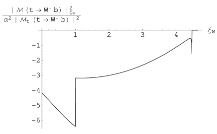
Figure 4: Gauge dependence of two-loop $|\cal{M}$$(t\rightarrow W^{+}b)|^{2}$ under the conventional wave-function renormalization prescription, where $\cal{M}$${}_{t}(t\rightarrow W^{+}b)$ is the tree-level amplitude.

Fig.3 and Fig.4 show the gauge dependence of the two physical results under the conventional wave-function renormalization prescription is order of $O(1)$ at two-loop level, so the conventional wave-function renormalization prescription will affect the veracity of physical results beyond one-loop level.

IV Conclusion

The new wave-function renormalization prescription proposed here is based on the pole mass renormalization prescription, in which WRC is extracted by expanding the particle’s propagator around its pole rather than its physical mass point as convention. The difference of the new WRC and the conventional WRC is gauge dependent for unstable particles beyond one-loop level. This will lead to some physical results gauge dependent under the conventional wave-function renormalization prescription beyond one-loop level.

Acknowledgments

The author thanks Prof. Cai-dian Lu for his devoted help.

References

(1)
H. Lehmann, K. Symanzik and W. Zimmermann, Nuovo Cimento 1 (1955) 1425.
(2)
A. Denner, Fortschr. Phys. 41 (1993) 307.
(3)
K.I. Aoki, Z. Hioki, M. Konuma, R. Kawabe, T. Muta, Prog. Theor. Phys. Suppl. 73 (1982) 1;
W.F.L. Hollik, Fortsch. Phys. 38 (1990) 165, Fortsch. Phys. 34 (1986) 687;
D. Espriu and J. Manzano, Phys. Rev. D 63 (2001) 073008;
B.A. Kniehl, A. Sirlin, Phys. Lett. B 530 (2002) 129;
F. Kleefeld, AIP Conf. Proc. 660 (2003) 325.
(4)
Yong Zhou, Mod. Phys. Lett. A, 21 (2006) 2763; hep-ph/0505138.
(5)
A.Sirlin, Phys. Rev. Lett. 67 (1991) 2127; Phys. Lett. B 267 (1991) 240;
R.G. Stuart, Phys. Lett. B 272 (1991) 353;
J.C. Breckenridge, M.J. Lavelle, T.G. Steele, Z. Phys. C 65 (1995) 155;
M. Passera, A. Sirlin, Phys. Rev. Lett. 77 (1996) 4146;
B.A. Kniehl, A. Sirlin, Phys. Rev. Lett. 81 (1998) 1373;
P. Gambino, P.A. Grassi, Phys. Rev. D 62 (2000) 076002;
P.A. Grassi, B.A. Kniehl and A. Sirlin, Phys. Rev. Lett. 86 (2001) 389;
M.L. Nekrasov, Phys. Lett. B 531 (2002) 225;
B.A. Kniehl, A. Sirlin, Phys. Lett. B 530 (2002) 129.
(6)
Yong Zhou, hep-ph/0508227; hep-ph/0510069.
(7)
Yong Zhou, J. Phys. G, 29 (2003) 1031.
(8)
D. Espriu, J. Manzano and P. Talavera, Phys. Rev. D66 (2002) 076002.
(9)
N.Cabibbo, Phys. Rev. Lett. 10, 531 (1963);
M.Kobayashi and K.Maskawa, Prog. Theor. Phys. 49 (1973) 652.
(10)
J. Kublbeck, M. Bohm, A. Denner, Comput. Phys. Commun. 60 (1990) 165;
G.J. van Oldenborgh, J.A.M. Vermaseren, Z. Phys. C46 (1990) 425;
T. Hahn, M. Perez-Victoria, Comput. Phys. Commun. 118 (1999) 153.
(11)
The European Physical Journal C, 15 (2000) 1-878.