SCET Analysis of $B\to K\pi$, $B\to K\bar{K}$, and $B\to\pi\pi$ Decays

Abstract

$B\to K\pi$ and related decays are studied in the heavy quark limit of QCD using the soft collinear effective theory (SCET). We focus on results that follow solely from integrating out the scale $m_{b}$, without expanding the amplitudes for the physics at smaller scales such as $\alpha_{s}(\sqrt{E_{\pi}\Lambda_{\rm QCD}})$. The reduction in the number of hadronic parameters in SCET leads to multiple predictions without the need of SU(3). We find that the CP-asymmetry in $B^{-}\to\pi^{0}K^{-}$ should have a similar magnitude and the same sign as the well measured asymmetry in $\bar{B}^{0}\to\pi^{+}K^{-}$. Our prediction for ${\rm Br}(K^{+}\pi^{-})$ exceeds the current experimental value at the $2\sigma$ level. We also use our results to determine the corrections to the Lipkin and CP-asymmetry sum rules in the standard model and find them to be quite small, thus sharpening their utility as a tool to look for new physics.

I Introduction

Two body nonleptonic decays are the most widely used processes to study CP violation in the $B$ system. Due to the large mass of the $B$-meson there is a plethora of open channels, each of which provides unique ways for testing the consistency of the standard model. For each channel observables include the CP averaged branching ratios (Br), direct CP asymmetry ($A_{CP}=-C$), and for certain neutral $B$ decays, the time dependent CP asymmetry ($S$). For the decays we are interested in

$${\rm Br}\equiv\frac{1}{\Gamma_{B}}\frac{s|\vec{p}|}{8\pi m_{B}^{2}}\Big{(}\frac{|{A}|^{2}+|\overline{A}|^{2}}{2}\Big{)}\,,\quad\lambda_{CP}=\frac{q}{p}\,\frac{\overline{A}}{A},$$ (1)

$$A_{\rm CP}\equiv\frac{|{A}|^{2}-|\overline{A}|^{2}}{|{A}|^{2}+|\overline{A}|^{2}}\,,\quad S=\frac{2\,{\rm Im}(\lambda_{CP})}{1+|{\lambda_{CP}}|^{2}}\,,$$

$$\frac{\Gamma_{B^{0}}(t)-\Gamma_{\bar{B}^{0}}(t)}{\Gamma_{B^{0}}(t)+\Gamma_{\bar{B}^{0}}(t)}\equiv-S\sin(\Delta m\,t)+C\cos(\Delta m\,t)\,,$$

where $A$ is the amplitude of the decay process $A=A(\bar{B}\to M_{1}M_{2})$, $\overline{A}$ is the amplitude for CP-conjugate process, and $q/p$ is the mixing parameter for $B^{0}-\bar{B}^{0}$ and/or $K^{0}-\bar{K}^{0}$ mixing. The other parameters in Eq.(1) are $|\vec{p}|$, the final meson momentum in the $B$ rest frame, $s$, a possible identical particle symmetry factor, and $\Delta m$, the difference between mass eigenstates in the neutral $B$ two-state system.

Using the unitarity of the CKM matrix to remove top-quark CKM elements, the amplitude for any decay can be written with the CKM elements factored out as

$$A=\lambda_{u}^{(f)}A_{u}+\lambda_{c}^{(f)}A_{c}\,,$$ (2)

where $\lambda_{p}^{(f)}=V_{pb}^{*}V_{pf}$. Theoretical predictions for the observables in (1) are often hampered by our ability to calculate $A_{u,c}$. In general the CP-asymmetries depend on the ratio of amplitudes $|A_{u}/A_{c}|$ and their relative strong phase $\delta$. In fact $A_{\rm CP}\propto\sin(\delta)$, and so non-negligible strong dynamics are required for the existence of a direct CP asymmetry.

The parameters $A_{u}$ and $A_{c}$ are in principle different for each decay channel. In order to accurately determine $A_{u}$ and $A_{c}$ we need model independent methods to handle the strong dynamics in these decays. All such methods involve systematic expansions of QCD in ratios of quark masses and the scale $\Lambda\simeq\Lambda_{\rm QCD}$ associated with hadronization. This includes flavor symmetries for the light quarks, SU(2) and SU(3), from $m_{q}/\Lambda\ll 1$, as well as expansions for the heavy $b$-quark from $\Lambda/m_{b}\ll 1$. For nonleptonic decays to two light mesons with energies $E_{m}\sim m_{b}/2$, kinematics implies that we must also expand in $\Lambda/E_{M}\ll 1$. A formalism for systematically expanding QCD in this fashion is the soft-collinear effective theory (SCET) SCET . In nonleptonic B-decays the expected accuracy of these expansions are

$${\rm SU(2)} \frac{m_{u,d}}{\Lambda}\sim 0.03\ll 1\,,$$ (3)

$${\rm SU(3)} \frac{m_{u,d}}{\Lambda}\ll 1,\ \frac{m_{s}}{\Lambda}\sim 0.3\ll 1\,,$$

$${\rm SCET} \frac{\Lambda}{E_{M}}\sim\frac{2\Lambda}{m_{b}}\sim 0.2\ll 1\,.$$

The flavor symmetries SU(2) and SU(3) provide amplitude relations between different nonleptonic channels, thereby reducing the number of hadronic parameters. The expansion in $\Lambda/m_{b}\sim\Lambda/E_{M}$ also reduces the number of hadronic parameters. In this case the expansion yields factorization theorems for the amplitudes in terms of moments of universal hadronic functions.

In this paper we study standard model predictions for $B\to K\pi$, $K\bar{K}$, and $\pi\pi$ decays. These channels provide 25 observables, of which 19 have been measured or bounded as summarized in Table 1. We make use of the expansions in Eq. (3), focusing on SCET. Our goal is to quantify the extent to which the current data agrees or disagrees with the standard model in the presence of hadronic uncertainties, and to provide a roadmap for looking for deviations in future precision measurements of these decays.

	${\rm Br}\times 10^{6}$	$A_{\rm CP}=-C$	$S$
$\pi^{+}\pi^{-}$	$5.0\pm 0.4$	$0.37\pm 0.10$	$-0.50\pm 0.12$
$\pi^{0}\pi^{0}$	$1.45\pm 0.29$	$0.28\pm 0.40$
$\pi^{+}\pi^{0}$	$5.5\pm 0.6$	$0.01\pm 0.06$	$-$
$\pi^{-}\bar{K}^{0}$	$24.1\pm 1.3$	$-0.02\pm 0.04$	$-$
$\pi^{0}K^{-}$	$12.1\pm 0.8$	$0.04\pm 0.04$	$-$
$\pi^{+}K^{-}$	$18.9\pm 0.7$	$-0.115\pm 0.018$	$-$
$\pi^{0}\bar{K}^{0}$	$11.5\pm 1.0$	$-0.02\pm 0.13$	$0.31\pm 0.26$
$K^{+}K^{-}$	$0.06\pm 0.12$
$K^{0}\bar{K}^{0}$	$0.96\pm 0.25$
$\bar{K}^{0}K^{-}$	$1.2\pm 0.3$		$-$

Table 1: Current $B\to\pi\pi$, $K\pi$, and $K\bar{K}$ data HFAG ; Babar ; Belle ; Cleo2 ; CDF . The $S$ for $\pi K$ is $S(\pi^{0}K_{S})$.

The SU(2) isospin symmetry is known to hold to a few percent accuracy, and thus almost every analysis of nonleptonic decays exploits isospin symmetry. (Electroweak penguin contributions are simply $\Delta I=1/2$ and $\Delta I=3/2$ weak operators, and are not what we mean by isospin violation.) Methods for determining or bounding $\alpha$ (or $\gamma$) using isospin have been discussed in GL ; isospinbound and are actively used in $B\to\pi\pi$ and $B\to\rho\rho$ decays. In $B\to\rho\rho$ this yields $\alpha_{\rho\rho}=96^{\circ}\pm 13^{\circ}$ HFAG . For $B\to\pi\pi$ this analysis has significantly larger errors, since the $A_{c}$ amplitudes are larger and the asymmetry $C(\pi^{0}\pi^{0})$ is not yet measured well enough to constrain the hadronic parameters. Isospin violating effects have been studied in isospinbreaking . For $B\to K\pi$ and $B\to K\bar{K}$ an SU(2) analysis is not fruitful since there are more isospin parameters than there are measurements, so further information about the hadronic parameters is mandatory.

In $B\to\pi\pi$, even if $C(\pi^{0}\pi^{0})$ were known precisely it would still be important to have more information about the amplitudes $A_{u}$ and $A_{c}$ than isospin provides. For example, isospin allows us to test whether $\gamma_{\pi\pi}$ differs from the value obtained by global fits CKMfitter ; UTfit ,

$$\gamma_{\rm\,global}^{\rm\,CKMfitter} =58.6^{\circ}{}^{+6.8^{\circ}}_{-5.9^{\circ}}\,,$$

$$\gamma_{\rm\,global}^{\rm\,UTfit} =57.9^{\circ}\pm 7.4^{\circ}\,.$$ (4)

However, a deviation in $\gamma$ is not the only way that new physics can appear in $B\to\pi\pi$ decays. Simply fitting the full set of SU(2) amplitudes can parameterize away a source of new physics. For example, Ref. Baek:2005cg has argued that it is impossible to see new physics in the $(\pi\pi)_{I=0}$ amplitudes in an isospin based fit. Thus, it is important to consider the additional information provided by SU(3) or factorization, since this allows us to make additional tests of the standard model. The expansion parameters here are larger, and so for these analyses it becomes much more important to properly assess the theoretical uncertainties in order to interpret the data.

The analysis of $B\to K\pi$ decays has a rich history in the standard model, provoked by the CLEO measurements CLEO that indicated that these decays are dominated by penguin amplitudes that were larger than expected. The dominance by loop effects makes these decays an ideal place to look for new physics effects. Some recent new physics analyses can be found in Refs. Kpinewphysics . This literature is divided on whether or not there are hints for new physics in these decays. The main obstacle is the assessment of the uncertainty of the standard model predictions from hadronic interactions.

Several standard model analyses based on the limit $m_{s}/\Lambda\ll 1$ (ie SU(3) symmetry) have been reported recently SU3gronau ; SU3buras ; SU3Li ; Suprun ; SU3Wu ; SU3other (see also su3 ; graphical2 ; burasfleischer for earlier work). In the $\Delta S=1$ decays the electroweak penguin amplitudes can not be neglected, since they are enhanced by CKM factors. Unfortunately the number of precise measurements makes it necessary to introduce additional “dynamical assumptions” to reduce the number of hadronic parameters beyond those in SU(3). In some cases efforts are made to estimate a subset of the SU(3) violating effects to further reduce the uncertainty. The dynamical assumptions rely on additional knowledge of the strong matrix elements and in the past were motivated by naive factorization or the large $N_{c}$ limit of QCD. Our current understanding of the true nature of factorization in QCD allows some of these assumptions to be justified by the $\Lambda/E_{M}$ expansion. However, it should be noted that a priori there is no reason to prefer these factorization predictions to others that follow from the $\Lambda/m_{b}$ expansion (such as the prediction that certain strong phases are small).

In Ref. SU3gronau a $\chi^{2}$-fit was performed with $\gamma$ as a fit parameter, including decays to $\eta$ and $\eta^{\prime}$. The result $\gamma=61^{\circ}\pm 11^{\circ}$ agrees well with global CKM fits. Here evidence for deviations from the standard model would show up as large contributions to the $\chi^{2}$. The most recent analysis Suprun has ${\rm Br}(K^{+}\pi^{-})$, ${\rm Br}(K^{0}\pi^{0})$, and $A_{\rm CP}(K^{0}\pi^{0})$ contributing $\Delta\chi^{2}=2.7$, $5.9$, and $2.9$ respectively, giving some hints for possible deviations from the standard model. Ref. SU3buras extracted hadronic paramters from $B\to\pi\pi$ decays, and used these results together with SU(3) and the neglect of exchange, penguin annihilation, and all electroweak penguin topologies except for the tree to make predictions for $B\to K\pi$ and $B\to K\bar{K}$ decays. They find large annihilation amplitudes, a large phase and magnitude for an amplitude ratio $\tilde{C}/\tilde{T}$ which is interpretted as large $P_{ut}$ penguin amplitudes. The deviation of ${\rm Br}(K^{+}\pi^{-})/{\rm Br}(\bar{K}^{0}\pi^{0})$ from standard model expectations was interpreted as evidence for new physics in electroweak penguins.

There has been tremendous progress over the last few years in understanding charmless two-body, non-leptonic $B$ decays in the heavy quark limit of QCD QCDF ; PQCD ; charmingpenguins ; earlier ; pipiChay ; bprs ; Bauer:2001cu ; Mantry:2003uz ; diff1 ; diff2 ; FH ; pQCDKpi ; BW ; BS ; Lee ; Kagan . In this limit one can prove factorization theorems of the matrix elements describing the strong dynamics in the decay into simpler structures such as light cone distribution amplitudes of the mesons and matrix elements describing a heavy to light transition QCDF (for earlier work see Refs. earlier ). It is very important that these results are obtained from a systematic expansion in powers of $\Lambda_{\rm QCD}/m_{b}$. The development of soft-collinear effective theory (SCET) SCET allowed these decays to be treated in the framework of effective theories, clarifying the separation of scales in the problem, and allowing factorization to be generalized to all orders in $\alpha_{s}$. In Ref. Bauer:2001cu a proof of factorization was given for $B\to DM^{-}$ type decays. Power corrections can also be investigated with SCET and in Ref. Mantry:2003uz a factorization theorem was proven for the color-suppressed $\bar{B}^{0}\to D^{0}M^{0}$ decays, and extended to isosinglet light mesons in Ref. Blechman:2004vc . Predictions from these results agree quite well with the available data, in particular the prediction of equal rates and strong phase shift for $D$ and $D^{*}$ channels.

Factorization for $B\to M_{1}M_{2}$ decays involves three distinct distance scales $m_{b}^{2}\gg E_{M}\Lambda\gg\Lambda^{2}$. For $B\to M_{1}M_{2}$ decays a factorization theorem was proposed by Beneke, Buchalla, Neubert and Sachrajda QCDF , often referred to as the QCDF result in the literature. Another proposal is a factorization formula which depends on transverse momenta, which is referred to as PQCD PQCD . The factorization theorem derived using SCET bprs ; pipiChay agrees with the structure of the QCDF proposal if perturbation theory is applied at the scales $m_{b}^{2}$ and $m_{b}\Lambda$. (QCDF treats the $c\bar{c}$ penguins perturbatively, while in our analysis they are left as a perturbative contribution plus an unfactorized large ${\cal O}(v)$ term.) Due to the charm mass scale the identification of a convergent expansion for the $c\bar{c}$ penguins remains unclear charmingpenguins ; FH ; diff1 ; diff2 . For further discussion see diff1 ; diff2 .) The SCET result improved the factorization formula by generalizing it to allow each of the scales $m_{b}^{2}$, $E_{M}\Lambda$, and $\Lambda^{2}_{\rm QCD}$ to be discussed independently. In particular, it was possible to show that a reduced set of universal parameters for these decays can already be defined after integrating out the scale $m_{b}^{2}$ bprs , opening up the ability to make predictions for nonleptonic decays without requiring an expansion in $\alpha_{s}(\sqrt{E\Lambda})$. (If the $m_{b}^{2}$ and $m_{b}\Lambda$ scales were separated in pQCD then this same result would be found for this first stage of factorization.) As a secondary step, additional predictions can be explored by doing a further expansion in $\alpha_{s}$ at the intermediate scale. The expense of the second expansion comes in principle with the benefit of a further reduction in the number of hadronic parameters and additional universality. In this paper we will explore the implications the first step of factorization has for $B\to K\pi$ decays.

There are several ways results from factorization can be used to analyze the data depending on i) whether perturbation theory is used at the intermediate $E_{M}\Lambda$ scale as mentioned above, and ii) whether light-cone sum rules, models, or data is used to determine the hadronic parameters. In the QCDF QCDF and PQCD PQCD analyses perturbation theory is used at the scale $E_{M}\Lambda$ and light-cone sum rules Ball ; Koj or simple estimates were used for numerical values of most of the hadronic parameters. Nonleptonic decay have also been studied with light-cone sum rules Khodj . With this input, all nonleptonic observables can be predicted and confronted with the experimental data. In both QCDF and PQCD a subset of power corrections are identified, parameterized in terms of new unknowns, and included in the numerical analysis. These power corrections are crucial to get reasonable agreement with the data. In these analyses it is sometimes difficult to distinguish between the model independent predictions from the heavy quark limit and the model dependent input from hadronic parameters. Ciucchini et al. have argued that so called charming penguins could be larger than expected and include unknowns to parameterize these effects charmingpenguins . Fitting the hadronic parameters to non-leptonic data in some channels and using the results to make predictions for other channels, as we advocate in this paper, has the advantage of avoiding model dependent input. Fits in QCDF have been performed in CKMfitter . So far restrictions on the size of leading and subleading hadronic parameters necessary to guarantee convergence have not been explored. Other fits based purely on isospin symmetry have been explored in isofits ; bprs .

In Ref. bprs ; gammafit ; GHLP the factorization theorem was used in a different way, focusing on $B\to\pi\pi$ decays. Here perturbation theory was only used at the $m_{b}^{2}$ scale and fits to nonleptonic data were performed for the hadronic parameters in the LO factorization theorem. The problematic contributions from charm-quark penguins were treated using only isospin symmetry. (This is also a good approach if power corrections spoil the expansion for this observable. Note that it avoids expanding the amplitude which has possible contamination from “chirally enhanced” power corrections QCDF .) Here we continue this program for $B\to K\pi$ and $B\to K\bar{K}$ decays (along with there comparison with $B\to\pi\pi$). For simplicity we refer to this as an “SCET” analysis, although it should be emphasized that other approaches to using the SCET-factorization theorem are possible. A key utility of factorization for nonleptonic decays is that the $\Lambda/E$ and $\alpha_{s}(m_{b})$ expansions are systematic and give us a method to estimate the theory uncertainty. Based on these uncertainties we investigate if the theory at leading order is able to explain the observed data. When deviations are found there are several possible explanations, all of which are interesting: either the expansions inherent in the theoretical analysis are suspect, or there are statistical fluctuations in the data, or we are seeing first hints of physics beyond the standard model.

This paper is organized as follows: In section II we discuss the theory input required to describe the decays of a $B$ meson to two light pseudoscalar mesons. We briefly review the electroweak Hamiltonian at $\mu=m_{b}$ and then we discuss the counting of the number of parameters required to describe these decays using SU(2), SU(3), and SCET analyses. We finish this section by giving a general parameterization of the decay amplitudes in SU(2). (In the appendix we give the relations between our parameters and the graphical amplitudes graphical1 ; graphical2 ; graphical3 .) In section III we give the expressions of the decay amplitudes in SCET. We begin by giving the general expressions at leading order in the power expansion, but correct to all orders in $\alpha_{s}$ and comment about new information that arises from combining these SCET relations with the SU(3) flavor symmetry. We then use the Wilson coefficients at leading order in $\alpha_{s}(m_{b})$ and give expressions for the decay amplitudes at that order. We finish this section with a discussion of our estimate of the uncertainties which arise from unknown ${\cal O}(\alpha_{s}(m_{b}))$ and ${\cal O}(\Lambda_{\rm QCD}/E)$ corrections. A detailed discussion of the implications of the SCET results is given in section IV. We emphasize that within factorization the ratios of color suppressed and color allowed amplitudes ($C/T$ and $EW^{C}/EW^{T}$) can naturally be of order unity at LO in the power counting, contrary to conventional wisdom bprs . We also perform an error analysis for the Lipkin and CP-sum rules in $B\to K\pi$ decays, and discuss predictions for the relative signs of the $CP$ asymmetries. We then review the information one can obtain from only the decays $B\to\pi\pi$, before we discuss in detail the implications of the SCET analysis for the decays $B\to K\pi$ and $B\to KK$.

II Theory Input

II.1 The electroweak Hamiltonian

The electroweak Hamiltonian describing $\Delta b=1$ transitions $b\to f$ is given by

$$H_{W}=\frac{G_{F}}{\sqrt{2}}\sum_{p=u,c}\lambda_{p}^{(f)}\Big{(}C_{1}O_{1}^{p}+C_{2}O_{2}^{p}+\!\!\!\sum_{i=3}^{10,7\gamma,8g}\!\!C_{i}O_{i}\Big{)},$$ (5)

where the CKM factor is $\lambda_{p}^{(f)}=V_{pb}V^{*}_{pf}$. The standard basis of operators are (with $O^{p}_{1}\leftrightarrow O^{p}_{2}$ relative to fullWilson )

$$O_{1}^{p}\!\! = \!\!(\overline{p}b)_{V\!-\!A}(\overline{f}p)_{V\!-\!A},\ \ O_{2}^{p}=(\overline{p}_{\beta}b_{\alpha})_{V\!-\!A}(\overline{f}_{\alpha}p_{\beta})_{V\!-\!A},$$

$$O_{3,4}\!\! = \!\!\big{\{}(\overline{p}b)_{V\!-\!A}(\overline{q}q)_{V\!-\!A}\,,(\overline{f}_{\beta}b_{\alpha})_{V\!-\!A}(\overline{q}_{\alpha}q_{\beta})_{V\!-\!A}\big{\}},$$

$$O_{5,6}\!\! = \!\!\big{\{}(\overline{f}b)_{V\!-\!A}(\overline{q}q)_{V\!+\!A}\,,(\overline{f}_{\beta}b_{\alpha})_{V\!-\!A}(\overline{q}_{\alpha}q_{\beta})_{V\!+\!A}\big{\}},$$

$$O_{7,8}\!\! = \frac{3e_{q}}{2}\!\!\big{\{}(\overline{f}b)_{V\!-\!A}(\overline{q}q)_{V\!+\!A}\,,(\overline{f}_{\beta}b_{\alpha})_{V\!-\!A}(\overline{q}_{\alpha}q_{\beta})_{V\!+\!A}\big{\}},$$

$$O_{9,10}\!\! = \frac{3e_{q}}{2}\!\!\big{\{}(\overline{f}b)_{V\!-\!A}(\overline{q}q)_{V\!-\!A}\,,(\overline{f}_{\beta}b_{\alpha})_{V\!-\!A}(\overline{q}_{\alpha}q_{\beta})_{V\!-\!A}\big{\}},$$

$$O_{7\gamma,8g}\!\! = \!\!-\frac{m_{b}}{8\pi^{2}}\ \overline{f}\,\sigma^{\mu\nu}\{eF_{\mu\nu},gG_{\mu\nu}^{a}T^{a}\}(1\!+\!\gamma_{5})b\,.$$ (6)

Here the sum over $q=u,d,s,c,b$ is implicit, $\alpha,\beta$ are color indices and $e_{q}$ are electric charges. The $\Delta S=0$ and $\Delta S=1$ effective Hamiltonian is obtained by setting $f=d$ and $f=s$ in Eqs. (5,II.1), respectively. The Wilson coefficients are known to NLL order fullWilson . At LL order taking $\alpha_{s}(m_{Z})=0.118$, $m_{t}=174.3$, and $m_{b}=4.8\,{\rm GeV}$ gives $C_{7\gamma}(m_{b})=-0.316$, $C_{8g}(m_{b})=-0.149$ and

$$C_{1-10}(m_{b})=\{1.107\,,-.249\,,.011\,,-.026\,,.008\,,-.031\,,$$

$$\ \ 4.9\!\times\!10^{-4}\,,4.6\!\times\!10^{-4}\,,-9.8\!\times\!10^{-3}\,,1.9\!\times\!10^{-3}\}\,.$$ (7)

Below the scale $\mu\sim m_{b}$ one can integrate out the $b\bar{b}$ pairs in the operators $O_{3-10}$. The remaining operators have only one $b$-quark field, and sums over light quarks $q=u,d,s,c$. This gives rise to a threshold correction to the Wilson coefficients,

$$C_{i}^{-}(m_{b})=C_{i}^{+}(m_{b})\Big{[}1+\frac{\alpha_{s}(m_{b})}{4\pi}\delta r_{s}^{T}+\frac{\alpha}{4\pi}\delta r_{c}^{T}\Big{]}\,,$$ (8)

where $C^{+}$ and $C^{-}$ are the Wilson coefficients with and without dynamical $b$ quarks, and $\delta r_{s}^{T}$ and $\delta r_{c}^{T}$ are given in Eqs. (VII.31) and (VII.32) of fullWilson . This changes the numerical values of the Wilson coefficients by less than 2%. Integrating out dynamical b quarks allows for additional simplifications for the electroweak penguin operators, since now for the flavor structure we have

$$\frac{3}{2}\,e_{q}(\bar{f}b)(\bar{q}q) =\frac{1}{2}\,(\bar{f}b)(2u\bar{u}-d\bar{d}-s\bar{s}+2c\bar{c})$$ (9)

$$\!\!\!\!=\frac{3}{2}\,(\bar{f}b)(u\bar{u})+\frac{3}{2}(\bar{f}b)(c\bar{c})-\frac{1}{2}\!\!\!\!\sum_{q=u,d,s,c}\!\!\!(\bar{f}b)(q\bar{q})\,.$$

The operators $O_{9}$ and $O_{10}$ have the regular $(V-A)\times(V-A)$ Dirac structure, and can therefore be written as linear combinations of the operators $O_{1-4}$,

$$O_{9} =\frac{3}{2}\,O_{2}^{u}+\frac{3}{2}\,O_{2}^{c}-\frac{1}{2}\,O_{3}\,,$$ (10)

$$O_{10} =\frac{3}{2}\,O_{1}^{u}+\frac{3}{2}\,O_{1}^{c}-\frac{1}{2}\,O_{4}\,.$$

This is not possible for the operators $O_{7}$ and $O_{8}$, which have $(V-A)\times(V+A)$ Dirac structure. Thus, integrating out the dynamical $b$ quarks removes two operators from the basis. To completely integrate out the dynamics at the scale $m_{b}$ we must match onto operators in SCET, as discussed in section III below.

II.2 Counting of Parameters

Without any theoretical input, there are 4 real hadronic parameters for each decay mode (one complex amplitude for each CKM structure) minus one overall strong phase. In addition, there are the weak CP violating phases that we want to determine. For $B\to\pi\pi$ decays there are a total of 11 hadronic parameters, while in $B\to K\pi$ decays there are 15 hadronic parameters.

Using isospin, the number of parameters is reduced. Isospin gives one amplitude relation for both the $\pi\pi$ and the $K\pi$ system, thus eliminating 4 hadronic parameters in each system (two complex amplitudes for each CKM structure). This leaves 7 hadronic parameters for $B\to\pi\pi$ and 11 for $B\to K\pi$. An alternative way to count the number of parameters is to construct the reduced matrix elements in SU(2). The electroweak Hamiltonian mediating the decays $B\to\pi\pi$ has up to three light up or down quarks. Thus, the operator is either $\Delta I=1/2$ or $\Delta I=3/2$. The two pions are either in an $I=0$ or $I=2$ state (the $I=1$ state is ruled out by Bose symmetry). This leaves 2 reduced matrix elements for each CKM structure, $\langle{\bf 0}||{\bf 1/2}||{\bf 1/2}\rangle$ and $\langle{\bf 2}||{\bf 3/2}||{\bf 1/2}\rangle$. For $B\to K\pi$ decays the electroweak Hamiltonian has either $\Delta I=0$ or $\Delta I=1$. The $K\pi$ system is either in an $I=1/2$ or $I=3/2$ state thus there are three reduced matrix elements per CKM structure, $\langle{\bf 3/2}||{\bf 1}||{\bf 1/2}\rangle$, $\langle{\bf 1/2}||{\bf 1}||{\bf 1/2}\rangle$ and $\langle{\bf 1/2}||{\bf 0}||{\bf 1/2}\rangle$. Finally, $K\bar{K}$ is either an $I=0$ or $I=1$, and there are again three reduced matrix elements per CKM structure, $\langle{\bf 0}||{\bf 1/2}||{\bf 1/2}\rangle$, $\langle{\bf 1}||{\bf 1/2}||{\bf 1/2}\rangle$, and $\langle{\bf 1}||{\bf 3/2}||{\bf 1/2}\rangle$.

The SU(3) flavor symmetry relates not only the decays $B\to\pi\pi$ and $B\to K\pi$, $B\to KK$, but also $B\to\pi\eta_{8}$, $B\to\eta_{8}K$ and $B_{s}$ decays to two light mesons. The decomposition of the amplitudes in terms of SU(3) reduced matrix elements can be obtained from Zeppenfeld ; SavageWise ; GrinsteinLebed . The Hamiltonian can transform either as a ${\bf\overline{3}}^{s}$, ${\bf\overline{3}}^{a}$, ${\bf 6}$ or ${\bf\overline{15}}$. Thus, there are 7 reduced matrix elements per CKM structure, $\langle{\bf 1}||{\bf\overline{3}}^{s}||{\bf 3}\rangle$, $\langle{\bf 1}||{\bf\overline{3}}^{a}||{\bf 3}\rangle$, $\langle{\bf 8}||{\bf\overline{3}}^{s}||{\bf 3}\rangle$, $\langle{\bf 8}||{\bf\overline{3}}^{a}||{\bf 3}\rangle$, $\langle{\bf 8}||{\bf 6}^{s}||{\bf 3}\rangle$, $\langle{\bf 8}||{\bf\overline{15}}^{s}||{\bf 3}\rangle$ and $\langle{\bf 27}||{\bf\overline{15}}^{s}||{\bf 3}\rangle$. The ${\bf\overline{3}}^{a}$ and ${\bf\overline{3}}^{s}$ come in a single linear combination so this leaves 20 hadronic parameters to describe all these decays minus 1 overall phase (plus additional parameters for singlets and mixing to properly describe $\eta$ and $\eta^{\prime}$). Of these hadronic parameters, only 15 are required to describe $B\to\pi\pi$ and $B\to K\pi$ decays (16 minus an overall phase). If we add $B\to KK$ decays then 4 more paramaters are needed (which are solely due to electroweak penguins). This is discussed further in section II.4.

	no			SCET	SCET
	expn.	SU(2)	SU(3)	+SU(2)	+SU(3)
$B\to\pi\pi$	11	7/5		4
$B\to K\pi$	15	11	15/13	+5(6)	4
$B\to K\bar{K}$	11	11	+4/0	+3(4)	+0

Table 2: Number of real hadronic parameters from different expansions in QCD. The first column shows the number of theory inputs with no approximations, while the next columns show the number of parameters using only SU(2), using only SU(3), using SU(2) and SCET, and using SU(3) with SCET. For the cases with two numbers, $\#/\#$, the second follows from the first after neglecting the small penguin coefficients, ie setting $C_{7,8}=0$. In SU(2) + SCET $B\to K\pi$ has 6 parameters, but 1 appears already in $B\to\pi\pi$, hence the $+5(6)$. The notation is analogous for the $+3(4)$ for $B\to K\bar{K}$.

The number of parameters that occur at leading order in different expansions of QCD are summarized in Table 2, including the SCET expansion. Here by SCET we mean after factorization at $m_{b}$ but without using any information about the factorization at $\sqrt{E\Lambda}$. The SCET results are discussed further in section III, but we summarize them here. The parameters with isospin+SCET are

$$\pi\pi: \{ \zeta^{B\pi}\!+\!\zeta_{J}^{B\pi},\beta_{\pi}\zeta_{J}^{B\pi},P_{\pi\pi}\}\,,$$ (11)

$$K\pi: \{ \zeta^{B\pi}\!+\!\zeta_{J}^{B\pi},\beta_{\bar{K}}\zeta_{J}^{B\pi},\zeta^{B\bar{K}}+\zeta_{J}^{B\bar{K}},\beta_{\pi}\zeta_{J}^{B\bar{K}},P_{K\pi}\}\,,$$

$$K\bar{K}: \{ \zeta^{B\bar{K}}+\zeta_{J}^{B\bar{K}},\beta_{K}\zeta_{J}^{B\bar{K}},P_{K\bar{K}}\}\,.$$

Here $P_{M_{1}M_{2}}$ are complex penguin amplitudes and the remaining parameters are real. In $B\to\pi\pi$ the moment parameter $\beta_{\pi}$ is not linearly independent from the parameters $\zeta^{B\pi}$ and $\zeta^{B\pi}_{J}$, and only the product $\beta_{\pi}\zeta_{J}^{B\pi}$ was counted as a parameter. In any case it is fairly well known from fits to $\gamma^{*}\gamma\to\pi^{0}$ pigammafit $3\beta_{\pi}\equiv\langle x^{-1}\rangle_{\pi}\simeq 3.2\pm 0.2$. In isospin + SCET $B\to K\pi$ has 6 parameters, but the first one listed in (11) appears already in $B\to\pi\pi$, hence the $+5$ in Table 2. If the ratio $\beta_{K}/\beta_{\pi}$ was known from elsewhere then one more parameter can be removed for $K\pi$ (leaving +4). For $B\to K\bar{K}$ we have $4$ SCET parameters. One of these appears already in $B\to K\pi$, hence the +3, and if $\beta_{K}/\beta_{\bar{K}}$ is known from other processes it would become $+2$.

Taking SCET + SU(3) we have the additional relations $\zeta^{B\pi}=\zeta^{BK}=\zeta^{B\bar{K}}$, $\zeta_{J}^{B\pi}=\zeta_{J}^{BK}=\zeta_{J}^{B\bar{K}}$, $\beta_{\pi}=\beta_{K}=\beta_{\bar{K}}$, and $A_{cc}^{\pi\pi}=A_{cc}^{K\pi}=A_{cc}^{K\bar{K}}$ which reduces the number of parameters considerably.

Note that there are good indications that the parameters $\zeta^{BM}$ and $\zeta^{BM}_{J}$ are positive numbers in the SCET factorization theorem. ($\beta_{K}$, $\beta_{\pi}$, $\beta_{\bar{K}}$ are also positive.) This follows from: i) the fact that $\zeta^{BM}+\zeta^{BM}_{J}$ are related to form factors for heavy-to-light transitions which with a suitable phase convention one expects are positive for all $q^{2}$, ii) that $\zeta^{BM}_{J}$ is positive (from the relatively safe assumption that radiative corrections at the scale $\sqrt{E\Lambda}$ do not change the sign of $\zeta_{J}^{M_{1}M_{2}}$ and that $\zeta_{J}\propto\beta_{\pi}\lambda_{B}>0$), and finally iii) that the fit to $B\to\pi\pi$ data gives $\zeta^{B\pi},\zeta_{J}^{B\pi}>0$ so that SU(3) implies $\zeta^{BK},\zeta_{J}^{BK}>0$. We will see that this allows some interesting predictions to be made even without knowing the exact values of the parameters.

In using the expansions in (3) it is important to keep in mind the hierarchy of CKM elements, and the rough hierarchy of the Wilson coefficients

$$C_{1}\gtrsim C_{2}\gg C_{3-6}\gg C_{9,10}\gtrsim C_{7,8}\,.$$ (12)

Some authors attempt to exploit the numerical values of the Wilson coefficients in the electroweak Hamiltonian to further reduce the number of parameters. A common example is the neglect of the coefficients $C_{7,8}$ relative to $C_{9,10}$. In Eq. (10) the electroweak penguin operators $O_{9}$ and $O_{10}$ were written as linear combinations of $O_{1-4}$. This implies that if one neglects the electroweak penguin operators $Q_{7}$ and $Q_{8}$, then no new operators are required to describe the EW penguin effects. In some cases this leads to additional simplifications. One can show that for $B\to\pi\pi$ decays the $\Delta I=3/2$ amplitudes multiplying the CKM structures $\lambda_{u}$ and $\lambda_{c}$ are identical graphical2 ; burasfleischer . Thus, SU(2) gives one additional relation between complex amplitudes in the $\pi\pi$ system, reducing the hadronic parameters to 5. For $B\to K\pi$ decays the operators giving rise to the $A_{3/2}$ reduced matrix elements are identical for the $\lambda_{u}$ and $\lambda_{c}$ CKM structures only if SU(3) flavor symmetry is used NeubertRosner . Thus, for these decays two hadronic parameters can be eliminated after using SU(3), leaving 13. Considering $B\to K\bar{K}$ adds two additional parameters. Note that dropping $C_{7,8}$ makes it impossible to fit for new physics in these coefficients. In our SCET analysis all contributions $C_{7-10}$ are included without needing additional hadronic parameters.

Finally, some analyses use additional “dynamical assumptions” and drop certain combinations of reduced matrix elements in SU(3). For example, the number of parameters is often reduced by neglecting parameters corresponding to the so called annihilation and exchange contributions.

II.3 General parameterization of the amplitudes using SU(2)

Using the SU(2) flavor symmetry, the most general amplitude parameterization for the decay $B\to\pi\pi$ is

$$A(\bar{B}^{0}\to\pi^{+}\pi^{-}) =-\lambda_{u}^{(d)}T_{\pi\pi}-\lambda_{c}^{(d)}P_{\pi\pi}$$ (13)

$$A(\bar{B}^{0}\to\pi^{0}\pi^{0}) =\!-\lambda_{u}^{(d)}C_{\pi\pi}-\!\lambda_{c}^{(d)}({EW}^{T}_{\pi\pi}-P_{\pi\pi})$$

$$\sqrt{2}A(B^{-}\to\pi^{-}\pi^{0}) =-\lambda_{u}^{(d)}(T_{\pi\pi}+C_{\pi\pi})-\lambda_{c}^{(d)}{EW}^{T}_{\pi\pi}$$

where we have used the unitarity of the CKM matrix $\lambda_{t}^{(f)}=-\lambda_{u}^{(f)}-\lambda_{c}^{(f)}$. The amplitude parameter ${EW}^{T}_{\pi\pi}$ receives contributions only through the electroweak penguin operators $O_{7-10}$. For $B\to K\pi$ decays we write

$$A(B^{-}\to\pi^{-}\bar{K}^{0}) = \lambda_{u}^{(s)}A_{K\pi}+\lambda_{c}^{(s)}P_{K\pi}$$ (14)

$$\sqrt{2}A(B^{-}\to\pi^{0}K^{-}) = -\lambda_{u}^{(s)}(C_{K\pi}+T_{K\pi}+A_{K\pi})$$

$$-\lambda_{c}^{(s)}(P_{K\pi}+{EW}^{T}_{K\pi})$$

$$A(\bar{B}^{0}\to\pi^{+}K^{-}) = -\lambda_{u}^{(s)}T_{K\pi}$$

$$-\lambda_{c}^{(s)}(P_{K\pi}+{EW}^{C}_{K\pi})$$

$$\sqrt{2}A(\bar{B}^{0}\to\pi^{0}\bar{K}^{0}) = -\lambda_{u}^{(s)}C_{K\pi}$$

$$+\lambda_{c}^{(s)}(P_{K\pi}-{EW}^{T}_{K\pi}+{EW}^{C}_{K\pi})$$

Finally for $B\to K\bar{K}$ decays there is no SU(2) relation between the amplitudes and we define

$$A(B^{-}\to K^{-}K^{0}) = \lambda_{u}^{(d)}A_{KK}+\lambda_{c}^{(d)}P_{KK}$$

$$A(\bar{B}^{0}\to K^{0}\bar{K}^{0}) = \lambda_{u}^{(d)}B_{KK}$$

$$+\lambda_{c}^{(d)}(P_{KK}+PA_{KK}+EW_{KK})$$

$$A(\bar{B}^{0}\to K^{-}K^{+}) = \lambda_{u}^{(d)}E_{KK}-\lambda_{c}^{(d)}PA_{KK}\,.$$ (15)

As mentioned before, after eliminating $\lambda_{t}^{(f)}$ there are four complex hadronic parameters for $B\to\pi\pi$ and six for $B\to K\pi$. The additional relation one obtains in the limit $C_{7,8}\to 0$ is

$${EW}^{T}_{\pi\pi} =\frac{3}{2}\frac{C_{9}+C_{10}}{C_{1}+C_{2}}({T}_{\pi\pi}+C_{\pi\pi})\,,$$ (16)

where we have neglected terms quadratic in $C_{9}$ or $C_{10}$.

The $EW$ amplitudes are purely from electroweak penguins, however there are also electroweak penguin contributions in the other amplitudes as discussed further in section III.4. Also, the hadronic parameters in Eqs. (13)-(II.3) are a minimal basis of isospin amplitudes, not graphical amplitude parameters. In the appendix we show how these amplitude parameters are related to the graphical amplitudes discussed in graphical1 ; graphical2 ; graphical3 .

II.4 Additional relations in the SU(3) limit

In the limit of exact SU(3) flavor symmetry the parameters in the $\pi\pi$ system and the $K\pi$ system satisfy the two simple relations graphical1 ; Zeppenfeld ; GrinsteinLebed

$$T_{\pi\pi}+C_{\pi\pi}=T_{K\pi}+C_{K\pi}$$

$${EW}^{T}_{\pi\pi}={EW}^{T}_{K\pi}\,.$$ (17)

Thus, the hadronic parameters in the combined $K\pi$, $\pi\pi$ system can be described by 8 complex parameters (15 real parameters after removing an overall phase), if no additional assumptions are made. A choice for these parameters is

$$T_{\pi\pi}\,,\quad C_{\pi\pi}\,,\quad P_{\pi\pi}\,,\quad A_{K\pi}\,,$$

$${EW}^{T}_{K\pi}\,,\quad{EW}^{C}_{K\pi},\quad\Delta C,\quad\Delta P$$ (18)

where we have defined

$$\Delta C \equiv C_{K\pi}-C_{\pi\pi}$$

$$\Delta P \equiv P_{\pi\pi}-P_{K\pi}$$ (19)

This can also be seen by relating these amplitude parameters directly to reduced matrix elements in SU(3), which can be done with the help of the results in Ref. GrinsteinLebed . As before, if the small Wilson coefficients $C_{7}$ and $C_{8}$ are neglected, we can again use the relation in Eq. (16) to eliminate one of the 8 complex hadronic parameters.

Four additional relations exist if the amplitudes for $B\to KK$ are included

$$A_{KK} = A_{K\pi}$$ (20)

$$P_{KK} = P_{K\pi}$$

$$E_{KK} = T_{K\pi}\!-\!T_{\pi\pi}=-\Delta C$$

$$PA_{KK} = P_{\pi\pi}\!-\!P_{K\pi}\!-\!EW^{C}_{K\pi}=\Delta P-EW^{C}_{K\pi}\,.$$

In the limit of vanishing Wilson coefficients $C_{7}$ and $C_{8}$ there are two additional relation graphical2

$$EW^{C}_{K\pi} = \frac{3}{4}\left[\frac{C_{9}-C_{10}}{C_{1}-C_{2}}\left(A_{K\pi}-T_{\pi\pi}+C_{K\pi}+B_{KK}\right)\right.$$

$$\left.-\frac{C_{9}+C_{10}}{C_{1}+C_{2}}\left(A_{K\pi}-T_{\pi\pi}+C_{K\pi}-2C_{\pi\pi}-B_{KK}\right)\right]$$

$$EW_{KK} = \frac{3}{2}\frac{C_{9}+C_{10}}{C_{1}+C_{2}}\left(B_{KK}-A_{KK}+E_{KK}\right)$$ (21)

II.5 Sum-Rules in $B\to K\pi$

In this section we review the derivation of two sum-rules for $B\to K\pi$, the Lipkin sum-rule Lipkin ; GR2 ; soni and CP sum-rule CPsum . Higher order terms are kept and will be used later on in assessing the size of hadronic corrections to these sum rules using factorization. To begin we rewrite the SU(2) parameterization of the amplitudes as

$$A(B^{-}\to\pi^{-}\bar{K}^{0})$$ (22)

$$=\lambda_{c}^{(s)}P_{K\pi}\Big{[}1-\frac{1}{2}\epsilon_{A}e^{-i\gamma}e^{i\phi_{A}}\Big{]}\,,$$

$$A(\bar{B}^{0}\to\pi^{+}K^{-})$$

$$=-\lambda_{c}^{(s)}P_{K\pi}\Big{[}1\!+\!\frac{1}{2}\big{(}\epsilon_{C}^{ew}e^{i\phi_{C}^{ew}}\!-\!\epsilon_{T}e^{i\phi_{T}-i\gamma}\big{)}\Big{]},$$

$$\sqrt{2}A(B^{-}\to\pi^{0}K^{-})$$

$$=-\lambda_{c}^{(s)}P_{K\pi}\Big{[}1\!+\!\frac{1}{2}\big{(}\epsilon_{T}^{ew}e^{i\phi_{T}^{ew}}\!-\!\epsilon e^{i\phi-i\gamma}\big{)}\Big{]},$$

$$\sqrt{2}A(\bar{B}^{0}\to\pi^{0}\bar{K}^{0})$$

$$=\lambda_{c}^{(s)}P_{K\pi}\Big{[}1\!-\!\frac{1}{2}\big{(}\epsilon_{ew}e^{i\phi_{ew}}\!-\!\epsilon_{C}e^{i\phi_{C}-i\gamma}\big{)}\Big{]},$$

where

$$\frac{1}{2}\,\epsilon_{T}e^{i\phi_{T}} =\bigg{|}\frac{\lambda_{u}^{(s)}}{\lambda_{c}^{(s)}}\bigg{|}\ \frac{(-T_{K\pi})}{P_{K\pi}}\,,$$ (23)

$$\ \ \frac{1}{2}\,\epsilon_{C}e^{i\phi_{C}} =\Big{|}\frac{\lambda_{u}^{(s)}}{\lambda_{c}^{(s)}}\Big{|}\ \frac{(-C_{K\pi})}{P_{K\pi}}\,,$$

$$\ \ \frac{1}{2}\,\epsilon_{A}e^{i\phi_{A}} =\Big{|}\frac{\lambda_{u}^{(s)}}{\lambda_{c}^{(s)}}\Big{|}\ \frac{(-A_{K\pi})}{P_{K\pi}}\,,$$

$$\frac{1}{2}\,\epsilon\>e^{i\phi} =\Big{|}\frac{\lambda_{u}^{(s)}}{\lambda_{c}^{(s)}}\Big{|}\ \frac{(-T_{K\pi}-C_{K\pi}-A_{K\pi})}{P_{K\pi}}\,,$$

and

$$\frac{1}{2}\,\epsilon_{T}^{ew}\>e^{i\phi_{T}^{ew}} =\frac{{EW}_{K\pi}^{T}}{P_{K\pi}}\,,$$ (24)

$$\frac{1}{2}\,\epsilon_{C}^{ew}\>e^{i\phi_{C}^{ew}} =\ \frac{{EW}_{K\pi}^{C}}{P_{K\pi}}\,,$$

$$\frac{1}{2}\,\epsilon_{ew}\>e^{i\phi_{ew}} =\frac{{EW}_{K\pi}^{T}-{EW}_{K\pi}^{C}}{P_{K\pi}}\,.$$

These parameters satisfy

$$\epsilon\>e^{i\phi} =\epsilon_{T}\,e^{i\phi_{T}}+\epsilon_{C}\,e^{i\phi_{C}}+\epsilon_{A}\,e^{i\phi_{A}}$$ (25)

$$\epsilon_{ew}e^{i\phi_{ew}} =\epsilon^{ew}_{T}e^{i\phi^{ew}_{T}}-\epsilon^{ew}_{C}e^{i\phi^{ew}_{C}}\,.$$

The non-electroweak $\epsilon$-parameters are suppressed by the small ratio of CKM factors $|\lambda_{u}^{(s)}/\lambda_{c}^{(s)}|\simeq 0.024$ but are then enhanced by a factor of $\sim 4$–$15$ by the ratio of hadronic amplitudes. The electroweak $\epsilon$-parameters are simply suppressed by their small Wilson coefficients and end up being similar in size to the non-electroweak $\epsilon$’s.

Next we define deviation parameters for the branching ratios

$$R_{1} =\frac{2{\rm Br}(B^{-}\to\pi^{0}K^{-})}{{\rm Br}(B^{-}\to\pi^{-}\bar{K}^{0})}-1\,,$$ (26)

$$R_{2} =\frac{{\rm Br}(\bar{B}^{0}\to\pi^{-}K^{+})\tau_{B^{-}}}{{\rm Br}(B^{-}\to\pi^{-}\bar{K}^{0})\tau_{B^{0}}}-1\,,$$

$$R_{3} =\frac{2{\rm Br}(\bar{B}^{0}\to\pi^{0}\bar{K}^{0})\tau_{B^{-}}}{{\rm Br}(B^{-}\to\pi^{-}\bar{K}^{0})\tau_{B^{0}}}-1\,,$$

and also rescaled asymmetries

$$\Delta_{1}=(1+R_{1})A_{\rm CP}(\pi^{0}K^{-})\,,$$ (27)

$$\Delta_{2}=(1+R_{2})A_{\rm CP}(\pi^{-}K^{+})\,,$$

$$\Delta_{3}=(1+R_{3})A_{\rm CP}(\pi^{0}\bar{K}^{0})\,,$$

$$\Delta_{4}=A_{\rm CP}(\pi^{-}\bar{K}^{0})\,.$$

The division by ${\rm Br}(\pi^{-}\bar{K}^{0})$ in the $\Delta_{i}$ asymmetries is not necessary but we find it convenient for setting the normalization. Expanding in $\epsilon_{A}$ we find that to second order in the $\epsilon$ parameters the $R_{i}$ are

$$R_{1} =\big{[}\epsilon_{T}^{ew}\cos\phi_{T}^{ew}\!-\!\epsilon\cos\phi\cos\gamma+\epsilon_{A}\cos\phi_{A}\cos\gamma\big{]}$$

$$+\!\Big{[}\frac{1}{4}\big{(}\epsilon^{2}\!+\!\epsilon_{T}^{ew\,2}\!-\!\epsilon_{A}^{2}\big{)}\!-\!\frac{1}{2}\>\epsilon\,\epsilon_{T}^{ew}\cos\gamma\cos(\phi\!-\!\phi_{T}^{ew})$$

$$\ \ \ +(\epsilon_{T}^{ew}\cos\phi_{T}^{ew}\!-\!\epsilon\cos\phi\cos\gamma)\,\epsilon_{A}\cos\phi_{A}\cos\gamma$$

$$\ \ \ +\epsilon_{A}^{2}\cos^{2}\phi_{A}\cos^{2}\gamma\Big{]},$$

$$R_{2} =\big{[}\epsilon_{C}^{ew}\cos\phi_{C}^{ew}\!-\!\epsilon_{T}\cos\phi_{T}\cos\gamma\!+\!\epsilon_{A}\cos\phi_{A}\cos\gamma\big{]}$$

$$+\!\Big{[}\frac{1}{4}\big{(}\epsilon_{T}^{2}\!+\!\epsilon_{C}^{ew\,2}\!-\!\epsilon_{A}^{2}\big{)}\!-\!\frac{1}{2}\>\epsilon_{T}\,\epsilon_{C}^{ew}\cos\gamma\cos(\phi_{C}^{ew}\!-\!\phi_{T})$$

$$\ \ \ +(\epsilon_{C}^{ew}\cos\phi_{C}^{ew}\!-\!\epsilon_{T}\cos\phi_{T}\cos\gamma)\,\epsilon_{A}\cos\phi_{A}\cos\gamma$$

$$\ \ \ +\epsilon_{A}^{2}\cos^{2}\phi_{A}\cos^{2}\gamma\Big{]},$$

$$R_{3} =\big{[}\!-\!\epsilon^{ew}\cos\phi_{ew}\!+\!\epsilon_{C}\cos\phi_{C}\cos\gamma\!+\!\epsilon_{A}\cos\phi_{A}\cos\gamma\big{]}$$

$$+\!\Big{[}\frac{1}{4}\big{(}\epsilon^{ew\,2}\!+\!\epsilon_{C}^{ew\,2}\!-\!\epsilon_{A}^{2}\big{)}\!-\!\frac{1}{2}\>\epsilon_{C}\,\epsilon^{ew}\cos\gamma\cos(\phi_{ew}\!-\!\phi_{C})$$

$$\ \ \ -(\epsilon^{ew}\cos\phi^{ew}\!-\!\epsilon_{C}\cos\phi_{C}\cos\gamma)\,\epsilon_{A}\cos\phi_{A}\cos\gamma$$

$$\ \ \ +\epsilon_{A}^{2}\cos^{2}\phi_{A}\cos^{2}\gamma\Big{]},$$ (28)

and the $\Delta_{i}$ are

$$\Delta_{1} =\sin\gamma\big{[}-\epsilon\sin\phi-\frac{1}{2}\,\epsilon\,\epsilon_{T}^{ew}\sin(\phi\!-\!\phi_{T}^{ew})\big{]}$$

$$\ \ \ \times\big{[}1+\epsilon_{A}\cos\phi_{A}\cos\gamma],$$

$$\Delta_{2} =\sin\gamma\big{[}-\epsilon_{T}\sin\phi_{T}-\frac{1}{2}\,\epsilon_{T}\,\epsilon_{C}^{ew}\sin(\phi_{T}\!-\!\phi_{c}^{ew})\big{]}$$

$$\ \ \ \times\big{[}1+\epsilon_{A}\cos\phi_{A}\cos\gamma],$$

$$\Delta_{3} =\sin\gamma\big{[}\epsilon_{C}\sin\phi_{C}-\frac{1}{2}\,\epsilon_{C}\,\epsilon^{ew}\sin(\phi_{C}\!-\!\phi_{ew})\big{]}$$

$$\ \ \ \times\big{[}1+\epsilon_{A}\cos\phi_{A}\cos\gamma],$$

$$\Delta_{4} =\sin\gamma\big{[}-\epsilon_{A}\sin\phi_{A}\big{]}\big{[}1+\epsilon_{A}\cos\phi_{A}\cos\gamma]\,.$$ (29)

Note that these rescaled CP-Asymmetries are independent of the electroweak penguin $\epsilon$’s at ${\cal O}(\epsilon)$. This is not true for the original asymmetries $A_{\rm CP}$.

Sum rules are derived by taking combinations of the $R_{i}$ and $\Delta_{i}$ which cancel the ${\cal O}(\epsilon)$ terms. The Lipkin sum rule is the statement that

$$R_{1}-R_{2}+R_{3}={\cal O}(\epsilon^{2})$$

$$=\frac{1}{4}\big{(}\epsilon^{2}-\epsilon_{T}^{2}+\epsilon_{C}^{2}-\epsilon_{A}^{2}+\epsilon_{T}^{ew\,2}-\epsilon_{C}^{ew\,2}+\epsilon^{ew\,2}\big{)}$$

$$+\epsilon_{A}^{2}\cos^{2}(\phi_{A})\cos^{2}(\gamma)-\frac{1}{2}\,\cos(\gamma)\big{[}\epsilon_{T}^{ew}\epsilon\cos(\phi\!-\!\phi_{T}^{ew})$$

$$-\epsilon_{T}\epsilon_{C}^{ew}\cos(\phi_{T}\!-\!\phi_{C}^{ew})+\epsilon_{C}\epsilon^{ew}\cos(\phi_{C}\!-\!\phi_{ew})\big{]}\,,$$ (30)

where we used the real part of Eq. (25). The CP-sum rule is the statement that using the imaginary part of Eq. (25) the ${\cal O}(\epsilon)$ terms cancel in the sum

$$\Delta_{1}-\Delta_{2}+\Delta_{3}-\Delta_{4}={\cal O}(\epsilon^{2})$$

$$=-\frac{1}{2}\sin(\gamma)\big{[}\epsilon_{T}^{ew}\epsilon\sin(\phi-\phi_{T}^{ew})-\epsilon_{T}\epsilon_{C}^{ew}\sin(\phi_{T}-\phi_{C}^{ew})$$

$$\ \ -\epsilon_{C}\epsilon^{ew}\sin(\phi_{C}-\phi_{ew})\big{]}\,.$$ (31)

The accuracy of these sum rules can be improved if we can determine these ${\cal O}(\epsilon^{2})$ terms using factorization. This is done in section IV.4.1.

III Amplitude parameters in SCET

III.1 General LO expressions

The factorization of a generic amplitude describing the decay of a $B$ meson to two light mesons, $B\to M_{1}M_{2}$, has been analyzed using SCET bprs . Here $M_{1}$ and $M_{2}$ are light (non-isosinglet) pseudoscalar or vector mesons. The SCET analysis involves two stages of factorization, first between the scales $\{m_{b}\mbox{ or }E_{M}\}^{2}\gg E_{M}\Lambda_{\rm QCD}$, and second between $E_{M}\Lambda_{\rm QCD}\gg\Lambda_{\rm QCD}^{2}$. Here we only consider the first stage of factorization where we integrate out the scales $\{m_{b},E_{M}\}$, and keep the most general parameterization for physics at lower scales. It was shown in Ref. bprs that a significant universality is already obtained after this first stage, in particular there is only one jet function which also appears in semileptonic decays to pseudoscalars and longitudinal vectors. This leads to the universality of the function we call $\zeta_{J}^{BM}(z)$. We note that this also proves that the second stage of matching is identical to that for the form factor, so the SCET results for form factors in Refs. ff can immediately be applied to nonleptonic decays if desired. A summary of the analysis of SCET operators and matrix elements is given in Appendix A.

After factorization at the scale $m_{b}$ the general LO amplitude for any $B\to M_{1}M_{2}$ process can be written

$$A\!\! = \!\!\frac{G_{F}m_{B}^{2}}{\sqrt{2}}\!\bigg{[}\bigg{\{}f_{M_{1}}\!\int_{0}^{1}\!\!\!\!du\,dz\,T_{1\!J}(u,z)\zeta^{BM_{2}}_{J}(z)\phi^{M_{1}}(u)$$ (32)

$$+f_{M_{1}}\zeta^{BM_{2}}\!\!\int_{0}^{1}\!\!\!\!du\,T_{1\zeta}(u)\phi^{M_{1}}(u)\bigg{\}}\!+\!\Big{\{}1\leftrightarrow 2\Big{\}}$$

$$+\lambda_{c}^{(f)}A_{c\bar{c}}^{M_{1}M_{2}}\bigg{]},$$

where $\zeta^{BM}$ and $\zeta^{BM}_{J}$ are non-perturbative parameters describing $B\to M$ transition matrix elements, and $A_{\rm c\bar{c}}^{M_{1}M_{2}}$ parameterizes complex amplitudes from charm quark contractions for which factorization has not been proven. Power counting implies $\zeta^{BM}\sim\zeta^{BM}_{J}\sim(\Lambda/Q)^{3/2}$. $T_{1\!J}(u,z)$ and $T_{1\zeta}(u)$ are perturbatively calculable in an expansion in $\alpha_{s}(m_{b})$ and depend upon the process of interest.

It is useful to define dimensionless hatted amplitudes

$$\hat{A}=\frac{A}{N_{0}}({\rm GeV}^{-1})\,,\quad N_{0}=\frac{G_{F}m_{B}^{2}}{\sqrt{2}}\,.$$ (33)

Using Eq. (32) we find that the amplitude parameters in the $B\to\pi\pi$ system are

$$\hat{T}_{\pi\pi} = -f_{\pi}\left[\langle c_{1u}+c_{4u}-c_{1t}^{ew}-c_{4t}\rangle_{\pi}\zeta^{B\pi}\right.$$

$$\left.\hskip 10.81218pt+\langle(b_{1u}+b_{4u}-b_{1t}-b_{4t})\zeta_{J}^{B\pi}\rangle_{\pi}\right]$$

$$\hat{C}_{\pi\pi} = -f_{\pi}\left[\langle c_{2u}-c_{2t}^{\rm ew}+c_{3t}^{\rm ew}+c_{4t}-c_{4u}\rangle_{\pi}\zeta^{B\pi}\right.$$

$$\left.\hskip 10.81218pt+\langle(b_{2u}-b_{2t}^{\rm ew}+b_{3t}^{\rm ew}+b_{4t}-b_{4u})\zeta_{J}^{B\pi}\rangle_{\pi}\right]$$

$$\hat{P}_{\pi\pi} = -A_{cc}^{\pi\pi}+f_{\pi}\left[\langle c_{1t}^{\rm ew}+c_{4t}\rangle_{\pi}\zeta^{B\pi}\right.$$

$$\left.\hskip 10.81218pt+\langle(b_{1t}^{\rm ew}+b_{4t})\zeta_{J}^{B\pi}\rangle_{\pi}\right]$$

$$\hat{EW}^{T}_{\pi\pi} = f_{\pi}\left[\langle c_{1t}^{\rm ew}+c_{2t}^{\rm ew}-c_{3t}^{\rm ew}\rangle_{\pi}\zeta^{B\pi}\right.$$ (34)

$$\left.\hskip 10.81218pt+\langle(b_{1t}^{\rm ew}+b_{2t}^{\rm ew}-b_{3t}^{\rm ew})\zeta_{J}^{B\pi}\rangle_{\pi}\right]\,.$$

For the $B\to K\pi$ system we find

$$\hat{T}_{K\pi} =-f_{K}\left[\langle c_{1u}-c_{1t}^{\rm ew}-c_{4t}+c_{4u}\rangle_{\bar{K}}\zeta^{B\pi}\right.$$

$$\left.\hskip 10.81218pt+\langle(b_{1u}-b_{1t}^{\rm ew}-b_{4t}+b_{4u})\zeta_{J}^{B\pi}\rangle_{\bar{K}}\right]$$

$$\hat{C}_{K\pi} =-f_{\pi}\left[\langle c_{2u}-c_{2t}^{\rm ew}+c_{3t}^{\rm ew}\rangle_{\pi}\zeta^{B\bar{K}}\right.$$

$$\left.\hskip 10.81218pt+\langle(b_{2u}-b_{2t}^{\rm ew}+b_{3t}^{\rm ew})\zeta_{J}^{B\bar{K}}\rangle_{\pi}\right]$$

$$+f_{K}\left[\langle c_{4t}-c_{4u}\rangle_{\bar{K}}\zeta^{B\pi}+\langle(b_{4t}-b_{4u})\zeta_{J}^{B\pi}\rangle_{\bar{K}}\right]$$

$$\hat{P}_{K\pi} =-A_{cc}^{K\pi}+f_{K}\left[\langle c_{4t}\rangle_{\bar{K}}\zeta^{B\pi}+\langle b_{4t}\zeta_{J}^{B\pi}\rangle_{\bar{K}}\right]$$

$$\hat{A}_{K\pi} =f_{K}\left[\langle c_{4t}-c_{4u}\rangle_{\bar{K}}\zeta^{B\pi}+\langle(b_{4t}-b_{4u})\zeta_{J}^{B\pi}\rangle_{\bar{K}}\right]$$

$$\hat{EW}^{T}_{K\pi} =f_{K}\left[\langle c_{1t}^{\rm ew}\rangle_{\bar{K}}\zeta^{B\pi}+\langle b_{1t}^{\rm ew}\zeta_{J}^{B\pi}\rangle_{\bar{K}}\right]$$

$$\hskip 19.91684pt+f_{\pi}\left[\langle c_{2t}^{\rm ew}-c_{3t}^{\rm ew}\rangle_{\pi}\zeta^{B\bar{K}}\right.$$

$$\left.\hskip 36.98866pt+\langle(b_{2t}^{\rm ew}-b_{3t}^{\rm ew})\zeta_{J}^{B\bar{K}}\rangle_{\pi}\right]$$

$$\hat{EW}^{C}_{K\pi} =f_{K}\left[\langle c_{1t}^{\rm ew}\rangle_{\bar{K}}\zeta^{B\pi}+\langle b_{1t}^{\rm ew}\zeta_{J}^{B\pi}\rangle_{\bar{K}}\right]\,.$$ (35)

Note that the dominant non-factorizable charm electroweak penguin contribution, is absorbed into $A_{cc}$. Finally, for the $B\to KK$ system we find

$$\hat{A}_{KK} =\hat{B}_{KK}$$ (36)

$$=f_{K}\left[\langle c_{4t}-c_{4u}\rangle_{K}\zeta^{B\bar{K}}+\langle\left(b_{4t}-b_{4u}\right)\zeta^{B\bar{K}}_{J}\rangle_{K}\right]$$

$$\hat{P}_{KK} =-A_{cc}^{K\bar{K}}+f_{K}\left[\langle c_{4t}\rangle_{K}\zeta^{B\bar{K}}+\langle b_{4t}\zeta^{B\bar{K}}_{J}\rangle_{K}\right]$$

$$\hat{E}_{KK} =\hat{PA}_{KK}=\hat{EW}_{KK}=0\,.$$

In Eqs. (III.1-36) we have defined

$$\langle c_{i}\rangle_{M} = \int_{0}^{1}\!\!du\,\,c_{i}(u)\phi_{M}(u)\,,$$ (37)

$$\langle b_{i}\,\zeta_{J}^{BM_{2}}\rangle_{M_{1}} = \int_{0}^{1}\!\!du\int_{0}^{1}\!\!dz\,\,b_{i}(u,z)\phi_{M_{1}}(u)\zeta_{J}^{BM_{2}}(z)\,.$$

We have also decomposed the Wilson coefficients of SCET operators defined in bprs as

$$c_{i}^{(f)} = \lambda_{u}^{(f)}c_{iu}+\lambda_{t}^{(f)}c_{it}$$

$$b_{i}^{(f)} = \lambda_{u}^{(f)}b_{iu}+\lambda_{t}^{(f)}b_{it}$$ (38)

and in some equations we have split the contributions from strong ($O_{3-6}$) and electroweak penguin operators ($O_{7-10}$) to the $c_{it}$ and $b_{it}$

$$c_{it} = c_{it}^{p}+c_{it}^{\rm ew}\,,$$

$$b_{it} = b_{it}^{p}+b_{it}^{\rm ew}\,.$$ (39)

Note that to all orders in perturbation theory one has graphical3

$$c_{1t}^{p}=c_{2t}^{p}=c_{3u}=c_{3t}^{p}=0$$

$$b_{1t}^{p}=b_{2t}^{p}=b_{3u}=b_{3t}^{p}=0\,.$$ (40)

All the hadronic information is contained in the SCET matrix elements $\zeta^{B\pi}$, $\zeta_{J}^{B\pi}$, $\zeta^{BK}$, $\zeta_{J}^{BK}$, $A_{cc}^{\pi\pi}$ and $A_{cc}^{K\pi}$, the decay constants $f_{\pi}$ and $f_{K}$, and the light cone distribution functions of the light mesons $\phi_{\pi}(x)$, $\phi_{K}(x)$, and $\phi_{\bar{K}}(x)$.

The Wilson coefficients $c_{i}$ and $b_{i}$ are insensitive to the long distance dynamics and can therefore be calculated using QCD perturbation theory in terms of the coefficients of the electroweak Hamiltonian, $C_{i}$. Any physics beyond the standard model which does not induce new operators in $H_{W}$ at $\mu=m_{W}$ will only modify the values of these Wilson coefficients, while keeping the expressions for the amplitude parameters in Eqs. (III.1–36) the same.

We caution that although the amplitudes $\hat{A}_{K\pi}$ and $\hat{A}_{KK}$ do get penguin contributions at this order, they will have subleading power contributions from operators with large Wilson coefficients that can compete. Therefore their leading order expressions presented here should not be used for numerical predictions. As mentioned earlier, the penguin amplitudes are kept to all orders in $\Lambda/E$. In all other amplitudes the power corrections are expected to be genuinely down by $\Lambda/E$ when the hadronic parameters are of generic size. In the observables explored numerically below it will be valid within our uncertainties to drop the small $\hat{A}_{K\pi}$ and $\hat{A}_{KK}$ amplitudes and so this point will not hinder us.

III.2 SU(3) limit in SCET

In the SU(3) limit the hadronic parameters for pions and kaons are equal. This implies that

$$\zeta^{B\pi}=\zeta^{B\bar{K}}\,,\qquad\quad\zeta_{J}^{B\pi}=\zeta_{J}^{B\bar{K}}\,,$$

$$\langle c_{i}\rangle_{K}=\langle c_{i}\rangle_{\pi}\,,$$ (41)

$$\langle b_{i}\zeta_{J}^{B\bar{K}}\rangle_{\pi}=\langle b_{i}\zeta_{J}^{B\pi}\rangle_{K}=\langle b_{i}\zeta_{J}^{B\pi}\rangle_{\pi}=\langle b_{i}\zeta_{J}^{B\bar{K}}\rangle_{K}\,.$$

Furthermore

$$A_{cc}^{K\pi}=A_{cc}^{\pi\pi}=A_{cc}^{K\bar{K}}\,.$$ (42)

To see this note that in SCET the light quark in the operator with two charm quarks is collinear and can therefore not be connected initial $B$ meson without further power suppression. Without the use of SCET this so called “penguin annihilation” contribution would spoil the relation in Eq. (42).

Using this we find two additional relations which are not true in a general SU(3) analysis but are true in the combined SCET + SU(3) limit

$$\Delta C = C_{K\pi}-C_{\pi\pi}=0\,,$$ (43)

$$\Delta P-{EW}^{C}_{K\pi} = P_{\pi\pi}-P_{K\pi}-{EW}^{C}_{K\pi}=0\,,$$

where the zeroes on the RHS are ${\cal O}(m_{s}/\Lambda)+{\cal O}(\Lambda/E)$. Using the SU(3) relation in Eq. (20) we see that these amplitudes are equal to “exchange” or “penguin annihilation” amplitudes that are power suppressed in SCET.

III.3 Results at LO in $\alpha_{s}(m_{b})$

While the $c_{i}$ are known at order $\alpha_{s}$, the $b_{i}$ are currently only known at tree level. For consistency, we thus keep only the tree level contributions to the $c_{i}$ as well. In this case they are independent of the light cone fraction $u$ and thus $c_{i}(u)\equiv c_{i}$, and there occurs a single nontrivial moment of the light-cone distribution function from the $b_{i}$ terms. Since the parameter $A_{cc}^{M_{1}M_{2}}\propto\alpha_{s}(2m_{c})$ it would be inconsistent to drop the $\alpha_{s}$ corrections in the penguin amplitudes. However, as long as we have the free complex parameter $A_{cc}^{M_{1}M_{2}}$ these corrections are simply absorbed when we work with the full penguin amplitudes $P_{M_{1}M_{2}}$ using only isospin symmetry. This is also true of chirally enhanced power corrections in $P_{M_{1}M_{2}}$.

Using LL values for the Wilson coefficients we find for the non-electroweak amplitudes at $\mu=m_{b}=4.8\,{\rm GeV}$

$$c_{1u} = C_{1}\!+\!\frac{C_{2}}{N_{c}}=1.025$$ (44)

$$c_{2u} = C_{2}\!+\!\frac{C_{1}}{N_{c}}=0.121$$

$$c_{4t}^{p} = -\Big{(}C_{4}+\frac{C_{3}}{N_{c}}\Big{)}+{\cal O}(C_{1}\alpha_{s})=0.022+{\cal O}(\alpha_{s})\,.$$

Here ${\cal O}(C_{1}\alpha_{s})$ indicate unsuppressed $\alpha_{s}$ corrections that were computed in Ref. QCDF and verified in pipiChay . The contributions from the operators $O_{7-10}$ give

$$c_{1t}^{\rm ew} = -\frac{3}{2}\Big{(}C_{10}\!+\!\frac{C_{9}}{N_{c}}\Big{)}=0.0021$$

$$c_{2t}^{\rm ew} = -\frac{3}{2}\Big{(}C_{9}\!+\!\frac{C_{10}}{N_{c}}\Big{)}=0.0138$$

$$c_{3t}^{\rm ew} = -\frac{3}{2}\Big{(}C_{7}+\frac{C_{8}}{N_{c}}\Big{)}=-0.0010$$

$$c_{4t}^{\rm ew} = \frac{1}{2}\Big{(}C_{10}+\frac{C_{9}}{N_{c}}\Big{)}=-0.00068\,.$$ (45)

The coefficients $b_{i}(u,z)$ are independent of the variable $z$ at leading order and we write $b_{i}(u,z)\equiv b_{i}(u)$. For the non-electroweak amplitudes we have

$$b_{1u}(u) = C_{1}+\Big{(}1+\frac{1}{\bar{u}}\Big{)}\frac{C_{2}}{N_{c}}$$

$$= 1.025-\frac{0.249}{3\bar{u}}$$

$$b_{2u}(u) = C_{2}+\Big{(}1+\frac{1}{\bar{u}}\Big{)}\frac{C_{1}}{N_{c}}$$

$$= 0.121+\frac{1.107}{3\bar{u}}$$

$$b_{4t}^{p}(u) = -C_{4}-\Big{(}1+\frac{1}{\bar{u}}\Big{)}\frac{C_{3}}{N_{c}}+{\cal O}(C_{1}\alpha_{s})$$

$$= 0.022-\frac{0.011}{3\bar{u}}+{\cal O}(\alpha_{s})$$

where ${\cal O}(C_{1}\alpha_{s})$ denotes unknown unsuppressed $\alpha_{s}$ corrections and $\bar{u}=1-u$. For the electroweak terms

$$b_{1t}^{\rm ew}(u) = -\frac{3}{2}\Big{[}C_{10}+\Big{(}1+\frac{1}{\bar{u}}\Big{)}\frac{C_{9}}{N_{c}}\Big{]}$$

$$= 0.0021+\frac{0.0147}{3\bar{u}}$$

$$b_{2t}^{\rm ew}(u) = -\frac{3}{2}\Big{[}C_{9}+\Big{(}1+\frac{1}{\bar{u}}\Big{)}\frac{C_{10}}{N_{c}}\Big{]}$$

$$= 0.0138-\frac{0.0029}{3\bar{u}}$$

$$b_{3t}^{\rm ew}(u) = -\frac{3}{2}\Big{[}C_{7}+\Big{(}1-\frac{1}{\bar{u}}\Big{)}\frac{C_{8}}{N_{c}}\Big{]}$$

$$= -0.00010+\frac{0.00069}{3u}$$

$$b_{4t}^{\rm ew}(u) = \frac{1}{2}\Big{[}C_{10}+\Big{(}1+\frac{1}{\bar{u}}\Big{)}\frac{C_{9}}{N_{c}}\Big{]}$$ (47)

$$= -0.00068-\frac{0.0049}{3\bar{u}}\,.$$

Note that only $b_{3t}^{\rm ew}$ involves $u$ and that this coefficient only appears convoluted with pions in Eqs. (III.1-36). For pions one can take $1/u\to 1/\bar{u}$ using charge conjugation and isospin. Since the $b$’s then only involve factors of $1/\bar{u}$ it is useful to define the nonperturbative parameters

$$\beta_{M}=\int_{0}^{1}\!\!\!du\>\frac{\phi_{M}(u)}{3\bar{u}}\,.$$ (48)

Using these values for the Wilson coefficients we obtain the amplitude parameters in terms of the non-perturbative parameters in the $\pi\pi$ system at $\mu=m_{b}$

$$\hat{T}_{\pi\pi} = -0.131\big{(}\zeta^{B\pi}+\zeta_{J}^{B\pi}\big{)}+0.031\,\beta_{\pi}\zeta_{J}^{B\pi}$$

$$\hat{C}_{\pi\pi} = -0.017\big{(}\zeta^{B\pi}+\zeta_{J}^{B\pi}\big{)}-0.144\,\beta_{\pi}\zeta_{J}^{B\pi}$$

$$\hat{EW}^{T}_{\pi\pi} = 0.0022\big{(}\zeta^{B\pi}+\zeta_{J}^{B\pi}\big{)}+0.0015\,\beta_{\pi}\zeta_{J}^{B\pi}$$

$$\hat{P}_{\pi\pi} = -A_{cc}^{\pi\pi}+0.0030\,\big{(}\zeta^{B\pi}+\zeta_{J}^{B\pi}\big{)}$$ (49)

$$-0.0002\,\beta_{\pi}\zeta_{J}^{B\pi}+\Delta_{\pi\pi}^{P}\,,$$

where $\Delta_{\pi\pi}^{P}$ is the additional perturbative correction from $a_{4t}$ and $b_{4t}$ at ${\cal O}(\alpha_{s}(m_{b}))$ which can involve larger Wilson coefficients like $C_{1,2}$. (We could also include large power corrections in $\Delta_{\pi\pi}^{P}$ assuming that such a subset could be uniquely identified in a proper limit of QCD.) We do not need knowledge of $\Delta_{\pi\pi}^{P}$ for our analysis since there are two unknowns in each of $\hat{P}_{\pi\pi}$ and $A_{cc}^{\pi\pi}$ and we will simply fit for $\hat{P}_{\pi\pi}$.

In the $K\pi$ system we find

$$\hat{T}_{K\pi} = -0.160\big{(}\zeta^{B\pi}+\zeta_{J}^{B\pi}\big{)}+0.040\,\beta_{K}\zeta_{J}^{B\pi}$$ (50)

$$\hat{C}_{K\pi} = -0.003\big{(}\zeta^{B\pi}+\zeta_{J}^{B\pi}\big{)}+0.003\,\beta_{K}\zeta_{J}^{B\pi}$$

$$-0.014\big{(}\zeta^{BK}+\zeta_{J}^{BK}\big{)}-0.146\,\beta_{\pi}\zeta_{J}^{BK}$$

$$\hat{EW}^{T}_{K\pi} = 0.0019\big{(}\zeta^{BK}+\zeta_{J}^{BK}\big{)}-0.0005\beta_{\pi}\zeta_{J}^{BK}$$

$$+0.0003\big{(}\zeta^{B\pi}+\zeta_{J}^{B\pi}\big{)}+0.0023\,\beta_{K}\zeta_{J}^{B\pi}$$

$$\hat{EW}^{C}_{K\pi} = 0.0003\big{(}\zeta^{B\pi}+\zeta_{J}^{B\pi}\big{)}+0.0023\,\beta_{K}\zeta_{J}^{B\pi}$$

$$\hat{P}_{K\pi} = -A_{cc}^{K\pi}+0.0034\big{(}\zeta^{B\pi}+\zeta_{J}^{B\pi}\big{)}$$

$$-0.0026\,\beta_{K}\zeta_{J}^{B\pi}+\Delta^{P}_{K\pi}$$

$$\hat{A}_{K\pi} = 0.0034\big{(}\zeta^{B\pi}+\zeta^{B\pi}_{J})-0.0026\,\beta_{K}\zeta_{J}^{B\pi}+\Delta^{A}_{K\pi}$$

where $\Delta_{K\pi}^{P}$ and $\Delta_{K\pi}^{A}$ are analogous corrections to $\Delta_{\pi\pi}^{P}$. For $P_{K\pi}$ the perturbative correction competes with $A_{cc}^{K\pi}$. For $\hat{A}_{K\pi}$ power corrections could be in excess of the leading order value, so that any numerical value for this amplitude is completely unreliable at the order we are working.

Finally for the $B\to K\bar{K}$ amplitudes that have a contribution from the LO factorization theorem we have

$$\hat{A}_{KK} =0.0034(\zeta^{BK}+\zeta_{J}^{BK})-0.0026\beta_{K}\zeta_{J}^{BK}$$

$$+{\cal O}(\alpha_{s})$$

$$\hat{P}_{KK} =-A_{cc}^{K\bar{K}}+0.0034(\zeta^{BK}+\zeta_{J}^{BK})$$

$$-0.0026\beta_{K}\zeta_{J}^{BK}+\Delta_{KK}^{P}$$ (51)

and $\hat{B}_{KK}=\hat{A}_{KK}$. Here the value of $\hat{A}_{KK}$ is not reliable, since it will have large ${\cal O}(C_{1}\Lambda/m_{b})$ power corrections that are likely to dominate.

III.4 SCET Relations for EW penguin amplitudes

Using the SCET results in the previous two sections it is simple to derive relations that give the electroweak penguin contributions in terms of tree amplitudes

$$\hat{T}_{M_{1}M_{2}}^{0} =\hat{T}_{M_{1}M_{2}}\big{|}_{C_{7-10}=0}\,,$$

$$\hat{C}_{M_{1}M_{2}}^{0} =\hat{C}_{M_{1}M_{2}}\big{|}_{C_{7-10}=0}\,.$$ (52)

Such relations are useful if one wishes to explore new physics scenarios that modify the electroweak penguin parameters $C_{7-10}$ in $H_{W}$. To separate out all electroweak penguin contributions in $B\to\pi\pi$ and using SCET together with isospin we define $\hat{EW}^{C}_{\pi\pi}$ by

$$\hat{T}_{\pi\pi}=\hat{T}^{0}_{\pi\pi}\!+\!{\hat{EW}}_{\pi\pi}^{C}\,, \hat{C}_{\pi\pi}=\hat{C}^{0}_{\pi\pi}\!+\!{\hat{EW}}_{\pi\pi}^{T}\!-\!{\hat{EW}}_{\pi\pi}^{C}\,,$$

$$\hat{P}_{\pi\pi}=\hat{P}^{0}_{\pi\pi}\!+\!{\hat{EW}}_{\pi\pi}^{C}\,.$$ (53)

At LO in SCET we find

$$\hat{EW}_{\pi\pi}^{C} =e_{1}\>\hat{T}_{\pi\pi}^{0}+e_{2}\>\hat{C}_{\pi\pi}^{0}\,,\$$

$$\hat{EW}_{\pi\pi}^{T} =e_{3}\>\hat{T}_{\pi\pi}^{0}+e_{4}\>\hat{C}_{\pi\pi}^{0}\,,\$$ (54)

where dropping $C_{3,4}$ relative to $C_{1,2}$ one finds

$$e_{1} =\frac{C_{10}C_{1}\!-\!C_{9}C_{2}}{C_{1}^{2}\!-\!C_{2}^{2}}=-2.9\!\times\!10^{-4}\,,$$ (55)

$$e_{2} =\frac{C_{9}C_{1}\!-\!C_{10}C_{2}}{C_{1}^{2}\!-\!C_{2}^{2}}=-8.9\!\times\!10^{-3}\,,$$

$$e_{3} =\frac{C_{1}(3C_{10}\!-\!3C_{7}\!-\!2C_{8}\!+\!3C_{9})\!-\!3C_{2}(C_{10}\!+\!C_{8}\!+\!C_{9})}{2(C_{1}^{2}\!-\!C_{2}^{2})}$$

$$=-1.5\times 10^{-2}\,,$$

$$e_{4} =\frac{-C_{2}(3C_{10}\!-\!3C_{7}\!-\!2C_{8}\!+\!3C_{9})\!+\!3C_{1}(C_{10}\!+\!C_{8}\!+\!C_{9})}{2(C_{1}^{2}\!-\!C_{2}^{2})}$$

$$=-1.3\times 10^{-2}\,.$$

The numbers quoted here are for the standard model LL coefficients.

For $B\to K\pi$ we separate out the electroweak penguin contributions by writing

$$\hat{T}_{K\pi}\!=\hat{T}^{0}_{K\pi}\!+\!\frac{2}{3}{\hat{EW}}_{\!K\pi}^{C}\,,\qquad\hat{A}_{K\pi}=\hat{P}^{0}_{K\pi}\!-\!\frac{1}{3}{\hat{EW}}_{\!K\pi}^{C}\,,$$

$$\hat{C}_{K\pi}=\hat{C}^{0}_{K\pi}\!+\!{\hat{EW}}_{\!K\pi}^{T}\!-\!\frac{2}{3}{\hat{EW}}_{\!K\pi}^{C}\,,$$

$$\hat{P}_{K\pi}=\hat{P}^{0}_{K\pi}\!-\!\frac{1}{3}{\hat{EW}}_{\!K\pi}^{C}\,,$$ (56)

and find that SCET+isospin gives

$$\hat{EW}_{K\pi}^{C} =\frac{f_{K}}{f_{\pi}}\Big{(}e_{5}\>\hat{T}_{\pi\pi}^{0}+e_{6}\>\hat{C}_{\pi\pi}^{0}\Big{)}+e_{7}\>\hat{T}_{K\pi}^{0}\,,\$$

where dropping $C_{3,4}$ relative to $C_{1,2}$

$$e_{5} =-\frac{3C_{1}(C_{1}C_{9}\!-\!C_{2}C_{10})}{2C_{2}(C_{1}^{2}\!-\!C_{2}^{2})}=-6.0\times 10^{-2}\,,$$

$$e_{6} =-\frac{3(C_{10}C_{2}-C_{9}C_{1})}{2(C_{1}^{2}\!-\!C_{2}^{2})}=-1.3\times 10^{-2}\,,$$

$$e_{7} =\frac{3C_{9}}{2C_{2}}=5.9\times 10^{-2}\,.$$ (57)

For the amplitude $EW^{T}_{K\pi}$ no such relation exists, if the inverse moments $\beta_{\pi}$ and $\beta_{K}$ are taken as unknowns. One can still use the SU(3) relation in Eq. II.4 to equate $EW^{T}$ in the $K\pi$ and $\pi\pi$ system.

III.5 Estimate of Uncertainties

These expressions of the amplitude parameters are correct at leading order in $\Lambda_{\rm QCD}/E_{\pi}$, and as we explained above, the complete set of Wilson coefficients is currently only available at tree level. Thus, any amplitude calculated from these SCET predictions has corrections at order $\alpha_{s}(m_{b})$ and $\Lambda_{\rm QCD}/E_{\pi}$. Using simple arguments based on dimensional analysis, we therefore expect corrections to any of these relations at the 20% level. We are working to all orders in $\alpha_{s}(\sqrt{\Lambda E})$, and so we avoid adding additional uncertainty from expanding at this scale.

Note that we have allowed for a general amplitude $P_{\pi\pi}$, which contributes to the reduced isospin matrix element $\langle{\bf 1/2}||{\bf 0}||{\bf 1/2}\rangle$ in the $K\pi$ system, and to the reduced isospin matrix element $\langle{\bf 0}||{\bf 1/2}||{\bf 1/2}\rangle$ in the $\pi\pi$ system. All power correction contributing to the same reduced matrix element will be absorbed into the value of the observable $P_{\pi\pi}$. In the following will thus fit directly for the parameters $P_{\pi\pi}$ and $P_{K\pi}$, which reduces the theoretical uncertainties significantly. This implies that the theoretical uncertainties on the amplitude parameters $\hat{P}_{\pi\pi}$, $\hat{P}_{K\pi}$, and $\hat{P}_{K\bar{K}}$ are $\sim 3\%$ from isospin rather than $\sim 20\%$. All other appreciable LO amplitude parameters are considered to have uncertainties at the 20% level.

Using this information, we can now estimate the size of corrections to the individual observables. For the decays $B\to\pi\pi$, contributions to the total amplitude from $\hat{P}_{\pi\pi}$ and other amplitudes are comparable, such that the whole amplitude receives ${\cal O}(20\%)$ corrections. This leads to corrections to the branching ratios and CP asymmetries in $B\to\pi\pi$ of order

$$\Delta{\rm Br}(B\to\pi\pi) \sim {\cal O}(40\%)$$

$$\Delta A_{\rm CP}(B\to\pi\pi) \sim {\cal O}(20\%)\,.$$ (58)

These large uncertainties can be avoided by relying on isospin to define most of the parameters in the fit, as was done in Ref. gammafit in the $\epsilon=0$ method for $\gamma$ which has significantly smaller theoretical uncertainties.

For $B\to K\pi$ decays, the CKM factors and sizes of Wilson coefficients give an enhancement of the amplitude parameter $\hat{P}_{K\pi}$ relative to the other amplitude parameters by a factor of order 10. Thus, the corrections to the total decay rates are suppressed by a factor of 10, while corrections to CP asymmetries, which require an interference between $\hat{P}_{K\pi}$ with other amplitudes, remain the same. This gives

$$\Delta{\rm Br}(B\to K\pi) \sim {\cal O}(5\%)$$

$$\Delta A_{\rm CP}(B\to K\pi) \sim {\cal O}(20\%)\,.$$ (59)

One exception is the CP asymmetry in $B\to K^{0}\pi^{-}$, which is strongly suppressed due to the smallness of the parameter $\hat{A}_{K\pi}$. At subleading order $\hat{A}_{K\pi}$ can receive corrections far in excess of the leading order value, such that any numerical value of this CP asymmetry is completely unreliable at the order we are working. We include these estimates of power corrections into all our discussions below.

IV Implications of SCET

There are several simple observations one can make from the LO SCET expressions of the amplitude parameters

1. For $\zeta^{BM_{i}}\sim\zeta_{J}^{BM_{i}}$ one finds that $B\to M_{1}M_{2}$ decays naturally have $\hat{C}_{M_{1}M_{2}}\sim\hat{T}_{M_{1}M_{2}}$ bprs , so there is no color suppression. If one instead takes $\zeta^{BM_{i}}\gg\zeta_{J}^{BM_{i}}$ as in Refs. QCDF ; PQCD then the “color suppressed” amplitude is indeed suppressed.

2. There is no relative phase between the amplitudes $C_{\pi\pi}$, $T_{\pi\pi}$, $T_{K\pi}$, $C_{K\pi}$, ${EW}^{T}_{K\pi}$ and ${EW}^{C}_{K\pi}$ and the sign and magnitude of these amplitudes can be predicted with SCET. This allows the uncertainty in the $K\pi$ sum-rules to be determined, as well as predictions for the relative signs of CP-asymmetries.

3. The contributions of electroweak penguins, $C_{7-10}$, can be computed without introducing additional hadronic parameters as discussed in Sec. III.4.

4. The amplitude $\hat{A}_{K\pi}$ is suppressed either by $\Lambda/m_{b}$, by small coefficients $C_{3,4}$, or by $\alpha_{s}(m_{b})$ compared with the larger $T_{K\pi}$ and $C_{K\pi}$ amplitudes

5. If one treats $\beta_{K}$ and $\beta_{\pi}$ as known, the amplitudes $\hat{T}_{K\pi}$ and $\hat{EW}^{C}_{K\pi}$ are determined entirely through the hadronic parameters describing the $B\to\pi\pi$ system, implying that the branching ratios and CP-asymmetries for $B\to K^{+}\pi^{-}$ and $B^{-}\to\bar{K}^{0}\pi^{-}$ only involve $2$ new parameters beyond $\pi\pi$.

6. In the combined SCET + SU(3) limit discussed in section III.2 the parameters $P_{\pi\pi}\simeq P_{K\pi}\simeq P_{K\bar{K}}$, so we expect similar complex penguin amplitudes in $B\to K\pi$, $B\to\pi\pi$, and $B\to K\bar{K}$.

Using these observations allows us to make important predictions for the observables, with and without performing fits to the data. Some of these have already been discussed and we elaborate on the remaining ones below.

IV.1 The ratio $C/T$ and $EW^{C}/EW^{T}$

We first describe in more detail the first point in the above list. Most literature has assumed that there is a hierarchy between the two amplitude parameters $C_{M_{1}M_{2}}$ and $T_{M_{1}M_{2}}$, ie. that $\hat{C}_{M_{1}M_{2}}\ll\hat{T}_{M_{1}M_{2}}$. This assumption is based on the fact that in naive factorization (in which $\zeta_{J}=0$) one has $C_{M_{1}M_{2}}/T_{M_{1}M_{2}}\sim c_{2u}/c_{1u}\sim 0.1$. The smallness of the ratio $c_{2u}/c_{1u}$ is due to the fact that the dominant Wilson coefficient $C_{1}$ of the electroweak Hamiltonian is multiplied by a factor of $1/N_{c}$ in $c_{2u}$, explaining the name “color suppressed” amplitude, plus additional accidental cancellations which reduce the value of this ratio below 1/3.

In SCET, however, the Wilson coefficients $b_{1,2}$ contribute with equal strength to the overall physical amplitude and can spoil the color suppression bprs . In the $b_{i}$ terms for $C_{M_{1}M_{2}}$ a factor of $1/N_{c}=1/3$ occurs, however the hadronic parameter in the numerator is the inverse moment of a light cone distribution function and is $\sim 3$. Thus numerically $\beta_{\pi,K}\simeq 1$, and setting $\beta_{\pi,K}=1$ for illustration we find

$$\hat{T}_{\pi\pi} = -0.131\zeta^{B\pi}-0.099\,\zeta_{J}^{B\pi}$$

$$\hat{C}_{\pi\pi} = -0.017\zeta^{B\pi}-0.160\,\zeta_{J}^{B\pi}$$

$$\hat{T}_{K\pi} = -0.160\,\zeta^{B\pi}-0.120\zeta_{J}^{B\pi}$$

$$\hat{C}_{K\pi} = -0.003\,\zeta^{B\pi}-0.001\,\zeta^{B\pi}_{J}$$ (60)

$$-0.014\zeta^{BK}-0.159\,\zeta_{J}^{BK}\,.$$

Thus, if $\zeta\sim\zeta_{J}$ it is easy to see that their is no “color suppression”. On the other hand if $\zeta\gg\zeta_{J}$ as chosen in Refs. QCDF ; PQCD then one would have significant color suppression.

From Eqs. (III.4-III.4) the size of the color-suppressed and color allowed electroweak penguin amplitudes in $\pi\pi$ and $K\pi$ are directly related to that of $C_{M_{1}M_{2}}$ and $T_{M_{1}M_{2}}$. Thus if $C_{M_{1}M_{2}}\sim T_{M_{1}M_{2}}$ then SCET predicts that $EW^{C}_{M_{1}M_{2}}\sim EW^{T}_{M_{1}M_{2}}$.

	Parameter	Measured value
	$m_{B}$	$(5279.4\pm 0.5)$ MeV pdg
	$\tau_{B^{0}}$	$(1.528\pm 0.009)$ ps HFAG
	$\tau_{B^{+}}$	$(1.643\pm 0.010)$ ps HFAG
	$\beta$	$0.379\pm 0.022$ HFAG
	$f_{\pi}$	$(130.7\pm 0.4)$ MeV pdg
	$f_{K}$	$(159.8\pm 1.5)$ MeV pdg
	$|V_{ud}|$	$0.9739\pm 0.0003$ ckm05
	$|V_{us}|$	$0.2248\pm 0.0016$ ckm05
	$|V_{cd}|$	$0.2261\pm 0.0010$ CKMfitter
	$|V_{cs}|$	$0.9732\pm 0.0002$ CKMfitter
	$|V_{cb}|$	$(41.6\pm 0.5)\times 10^{-3}$ HFAG ; globalfit
	$|V_{ub}|^{\rm incl}$	$(4.39\pm 0.34)\times 10^{-3}$ HFAG ; theoryVub
	$|V_{ub}|^{\rm excl}$	$(3.92\pm 0.52)\times 10^{-3}$ Lattice ; agrs ; LP
	$|V_{ub}|^{\rm global}_{\rm CKM}$	$(3.53\pm 0.22)\times 10^{-3}$ CKMfitter
	$|V_{ub}|^{\rm here}$	$(4.25\pm 0.34)\times 10^{-3}$

Table 3: Summary of well measured input parameters. For our central value for $|V_{ub}|$ we use a weighted average of the inclusive HFAG and exclusive LP with a slightly inflated error. Use $m_{t}=174.3\,{\rm GeV}$.

IV.2 $B\to\pi\pi$ with Isospin and ${\rm Im}(C_{\pi\pi}/T_{\pi\pi})=0$

Using only SU(2) there are a total of 5 hadronic parameters describing the decays $B\to\pi\pi$, in addition to a weak phase. The 6 measurements allow in principle to determine all of these parameters as was first advocated by Gronau and London GL . Unfortunately, the large uncertainties in the direct CP asymmetry of $\bar{B}^{0}\to\pi^{0}\pi^{0}$ do not allow for a definitive analysis at the present time (ie. it currently gives $65^{\circ}<\alpha<200^{\circ}$ CKMfitter ). It was shown in Ref. gammafit that one can use SCET to eliminate one of the 5 hadronic SU(2) parameters, since $\epsilon={\rm Im}(C_{\pi\pi}/T_{\pi\pi})\simeq 0$, and then directly fit for the remaining four hadronic parameters and the weak angle $\gamma$, which substantially reduces the uncertainty. Using the most recent data shown in section I, we find

$$\gamma^{\pi\pi}=83.0^{\circ}{}^{+7.2^{\circ}}_{-8.8^{\circ}}\pm 2^{\circ}$$ (61)

where the first error is from the experimental uncertainties, while the second uncertainty is an estimate of the theoretical uncertainties from the expansions in SCET, estimated by varying $\epsilon=\pm 0.2$ as explained in Ref. gammafit . This value is in disagreement with the results from a global fit to the unitarity triangle

$$\gamma_{\rm\,global}^{\rm\,CKMfitter} =58.6^{\circ}{}^{+6.8^{\circ}}_{-5.9^{\circ}}\,,$$

$$\gamma_{\rm\,global}^{\rm\,UTfit} =57.9^{\circ}\pm 7.4^{\circ}\,,$$ (62)

at the $2$-$\sigma$ level. A more sophisticated statistical analysis can be found in Ref. GHLP . The errors in Eq. (61) are slightly misleading because they do not remain Gaussian for larger $\epsilon$. At $\epsilon=0.3$ the deviation drops to $1.5$-$\sigma$, and at $\epsilon=0.4$ it drops to $0.5$-$\sigma$. The result in Eq. (61) is consistent with the direct measurement of this angle which has larger errors HFAG

$$\gamma^{DK}=63^{\circ}{}^{+15^{\circ}}_{-12^{\circ}}\,.\qquad$$ (63)

It is interesting to note that the global fit for $\beta$ plus the inclusive determination of $|V_{ub}|$ in table 3 also prefers larger values of $\gamma$ as shown in Fig. -419. It will be quite interesting to see how these hints of discrepancies are sharpened or clarified in the future. In the remainder of this paper, we will show results for $\gamma=83^{\circ}$ and $\gamma=59^{\circ}$ to give the reader an indication of the $\gamma$ dependence of our results.

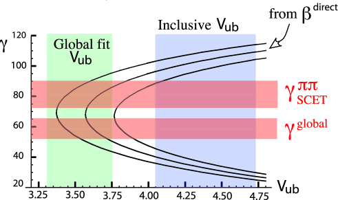
Figure -419: Comparison of constraints on $V_{ub}$ and $\gamma$ from i) the direct measurement of $\beta$, ii) current HFAG value for inclusive $|V_{ub}|$, iii) global fit value of $\gamma$, iv) $|V_{ub}|$ as output from the global fit  HFAG ; CKMfitter , and v) results for $\gamma$ from the small $\epsilon$ analysis of $B\to\pi\pi$ decays gammafit . All errors bands are $1$-$\sigma$.

The phase of the amplitude $A_{cc}^{\pi\pi}$ is mostly determined from the CP asymmetries in $B\to\pi^{+}\pi^{-}$. In particular, as can be seen from the general parameterization of the amplitudes in Eq. (13), the sign of the direct CP asymmetry $C({\pi^{+}\pi^{-}})$ is correlated with the relative sign between $\hat{P}_{\pi\pi}$ and $\hat{T}_{\pi\pi}$ and the sign of the asymmetry $C({\pi^{0}\pi^{0}})$ with that between $\hat{C}_{\pi\pi}$ and $\hat{P}_{\pi\pi}$. Since there is no relative phase between the amplitudes $\hat{C}_{\pi\pi}$ and $\hat{T}_{\pi\pi}$ at LO in SCET, the sign of the direct CP asymmetry in $B\to\pi^{0}\pi^{0}$ is thus expected to be positive based on the negative experimental value for $C(\pi^{+}\pi^{-})$ GHLP . This expectation is in disagreement with the direct measurement shown in Table 1. Using the values of the hadronic parameters from the previous fit we find for $\gamma=83^{\circ}$

$$C(\pi^{0}\pi^{0})=0.49\pm 0.12\pm 0.23\,,$$ (64)

while for $\gamma=59^{\circ}$ we find

$$C(\pi^{0}\pi^{0})=0.61\pm 0.19\pm 0.19\,.$$ (65)

These values are $1.7\sigma$ from the measured value, if we add the theoretical and experimental errors in quadrature.

IV.3 The decays $B\to\pi\pi$ in SCET

For $\gamma=83^{\circ}$ a fit of the four SCET parameters to the $B\to\pi\pi$ data excluding the direct CP asymmetry in $B\to\pi^{0}\pi^{0}$ gives

$$\zeta^{B\pi} =(0.088\pm 0.019\pm 0.045)\ \Big{(}\frac{4.25\times 10^{-3}}{|V_{ub}|}\Big{)}$$

$$\zeta_{J}^{B\pi} =(0.085\pm 0.016\pm 0.031)\ \Big{(}\frac{4.25\times 10^{-3}}{|V_{ub}|}\Big{)}$$

$$10^{3}\hat{P}^{\pi\pi} =(5.5\pm 0.8\pm 1.3)e^{i(151\pm 8\pm 6)^{\circ}},$$ (66)

while for $\gamma=59^{\circ}$ we find

$$\zeta^{B\pi} =(0.093\pm 0.023\pm 0.035)\ \Big{(}\frac{4.25\times 10^{-3}}{|V_{ub}|}\Big{)}$$

$$\zeta_{J}^{B\pi} =(0.10\pm 0.016\pm.022)\ \Big{(}\frac{4.25\times 10^{-3}}{|V_{ub}|}\Big{)}$$

$$10^{3}\hat{P}^{\pi\pi} =(2.6\pm 0.9\pm 0.8)e^{i(103\pm 19\pm 16)^{\circ}}\!.$$ (67)

The first error is purely from the uncertainties in the experimental data, while the second error comes from adding our estimate of the theory uncertainties discussed in section III.5. For both values of $\gamma$ one finds that $|P/T|\sim 0.25$. Note that this ratio of $P/T$ does not include the ratio of the CKM factors. The ratio relevant for the decays is $|\lambda_{c}^{(d)}/\lambda_{u}^{(d)}||P/T|\sim 0.6$.

It is interesting to compare the result for $\hat{P}^{\pi\pi}$ extracted from the data with that from the purely perturbative penguin computed in Ref. QCDF (in two scenarios for the input parameters),

$$10^{3}\hat{P}^{\rm default}_{\rm QCDF} =-1.0-[0.1+0.3i+\ldots]$$ (68)

$$-(1.7+0.0X_{H}+.047X_{A}^{2})-\{0.3+0.1i\}$$

$$=-3.1-0.4i-0.047X_{A}^{2}\,,$$

$$10^{3}\hat{P}^{\rm S2}_{\rm QCDF} =-0.9-[0.0+0.1i+\ldots]$$

$$-(2.0+0.0X_{H}+.063X_{A}^{2})-\{0.3+0.3i\}$$

$$=-3.2-0.4i-0.063X_{A}^{2}\,,.$$

Here the terms $[\ldots]$ are $\alpha_{s}(m_{b})$ corrections, the terms $(\ldots)$ are chirally enhanced power corrections with parameters $X_{H}$ and $X_{A}$, and $\{\ldots\}$ are perturbative corrections to these. We observe that the magnitude of the perturbative $\pi\pi$ penguin is of similar size to that from the data for $\gamma=59^{\circ}$, but has a small strong phase is in contrast to the large strong phase seen in the data.

The correlation between $\zeta^{B\pi}$ and $\zeta_{J}^{B\pi}$ in Eqs. (IV.3,IV.3) is about $-0.8$, so that the heavy-to-light form factor, which is given by the sum of these two parameters is determined with much smaller uncertainties than one would obtain by naively adding the two individual errors in quadrature. For $\gamma=83^{\circ}$ we find

$$F^{B\pi}(0)=(0.17\pm 0.01\pm 0.03)\ \Big{(}\frac{4.25\times 10^{-3}}{|V_{ub}|}\Big{)}$$ (69)

while for $\gamma=59^{\circ}$ we find

$$F^{B\pi}(0)=(0.19\pm 0.01\pm 0.03)\ \Big{(}\frac{4.25\times 10^{-3}}{|V_{ub}|}\Big{)}$$ (70)

IV.4 The decays $B\to K\pi$

For these decays the penguin amplitudes are enhanced by the ratio of CKM matrix elements $|\lambda_{c}^{(s)}/\lambda_{u}^{(s)}|\sim 40$. Thus, the relevant ratio of penguin to tree amplitudes is $|\lambda_{c}^{(s)}/\lambda_{u}^{(s)}||P/T|\sim 10$ and the $B\to K\pi$ decays are penguin dominated. If one were to only keep the penguin contributions to these decays the relative sizes of the branching ratios would be determined by simple Clebsch-Gordon coefficients

$${\rm Br}(\pi^{0}\bar{K}^{0})\simeq{\rm Br}(\pi^{0}K^{-})\simeq\frac{{\rm Br}(\pi^{+}K^{-})}{2}\simeq\frac{{\rm Br}(\pi^{-}\bar{K}^{0})}{2}\,.$$ (71)

Deviations from this relation are determined at leading order in the power counting by the non-perturbative parameters $\zeta^{BM}$ and $\zeta_{J}^{BM}$. To see how well the current data constrains deviations from this result we can look at the following ratios of branching fractions

$$R_{1} =\frac{2{\rm Br}(B^{-}\to\pi^{0}K^{-})}{{\rm Br}(B^{-}\to\pi^{-}\bar{K}^{0})}-1=0.004\pm 0.086\,,$$ (72)

$$R_{2} =\frac{{\rm Br}(\bar{B}^{0}\to\pi^{-}K^{+})\tau_{B^{-}}}{{\rm Br}(B^{-}\to\pi^{-}\bar{K}^{0})\tau_{B^{0}}}-1=-0.157\pm 0.055\,,$$

$$R_{3} =\frac{2{\rm Br}(\bar{B}^{-}\to\pi^{0}\bar{K}^{0})\tau_{B^{-}}}{{\rm Br}(\bar{B}^{0}\to\pi^{-}\bar{K}^{0})\tau_{B^{0}}}-1=0.026\pm 0.105\,,$$

and the rescaled asymmetries

$$\Delta_{1}=(1+R_{1})A_{\rm CP}(\pi^{0}K^{-})=0.040\pm 0.040\,,$$ (73)

$$\Delta_{2}=(1+R_{2})A_{\rm CP}(\pi^{-}K^{+})=-0.097\pm 0.016\,,$$

$$\Delta_{3}=(1+R_{3})A_{\rm CP}(\pi^{0}\bar{K}^{0})=-0.021\pm 0.133\,,$$

$$\Delta_{4}=A_{\rm CP}(\pi^{-}\bar{K}^{0})=-0.02\pm 0.04\,.$$ (74)

These ratios have been defined by normalizing each branching ratio to the decay $B^{-}\to\pi^{0}\bar{K}^{0}$. If we drop the small amplitude parameter $A_{K\pi}$ then this channel measures the penguin,

$$A(B^{-}\to\pi^{-}\bar{K}^{0})=\lambda_{c}^{(s)}P_{K\pi}\,,$$ (75)

and the direct CP asymmetry is expected to be small.

A simple test for the consistency of the $K\pi$ data is given by the Lipkin sum-rule for branching ratios Lipkin , and a sum-rule for the CP-asymmetries CPsum

$$R_{1}-R_{2}+R_{3}=0\,,\quad\Delta_{1}-\Delta_{2}+\Delta_{3}-\Delta_{4}=0\,,$$ (76)

which are both second order in the ratio of small to large amplitudes as discussed in section II.5. The current data gives

$$R_{1}-R_{2}+R_{3}=(0.19\pm 0.15)^{\rm expt}\,,$$

$$\Delta_{1}-\Delta_{2}+\Delta_{3}-\Delta_{4}=(0.14\pm 0.15)^{\rm expt}\,.$$ (77)

Thus, so far this global test does not show a deviation from the expectation.

SCET provides us with additional tests for the $K\pi$ data. It turns out that the current data is not precise enough to determine the values of $\zeta^{BK}$ and $\zeta_{J}^{BK}$. These two parameters only contribute to the two decays $B^{-}\to\pi^{0}K^{-}$ and $\bar{B}^{0}\to\pi^{0}\bar{K}^{0}$, which have neutral pions and larger experimental uncertainties. As we will explain, the data on these decays seems to favor a negative value of $\zeta_{J}^{BK}$, but that would imply a negative value for $\lambda_{B}$, the first inverse moment of the $B$ meson wave function, contrary to any theoretical prejudice. One can use the fact that the only sizeable strong phase is in the value of the parameter $A_{cc}^{K\pi}$ to determine the predicted size of the deviations from the above relations and also the signs and hierarchy for the CP asymmetries.

IV.4.1 Sum-Rules in $B\to K\pi$

In SCET positive values of $\zeta^{BM}$ and $\zeta_{J}^{BM}$ imply that the phase of $-T_{K\pi}$, $-C_{K\pi}$, ${EW}_{K\pi}^{C,T}$, and ${EW}_{K\pi}^{T}-{EW}_{K\pi}^{C}$ are the same. This can be seen from Eqs.(III.3-50). Therefore this implies that these amplitudes have a common strong phase $\delta$ relative to the penguin $\hat{P}_{K\pi}$. Using the notation and results from section II.5 we have

$$\phi_{T}=\phi_{C}=\phi=\phi_{T}^{ew}=\phi_{C}^{ew}=\phi_{ew}=\delta\,.$$ (78)

At LO in SCET one can drop the $A_{K\pi}$ amplitude ($\epsilon_{A}=0$) and write

$$A(\bar{B}^{0}\to\pi^{-}\bar{K}^{0}) =\lambda_{c}^{(s)}P_{K\pi}\,,$$ (79)

$$A(\bar{B}^{0}\to\pi^{+}K^{-}) =-\lambda_{c}^{(s)}P_{K\pi}\Big{[}1\!+\!\frac{e^{i\delta}}{2}\big{(}\epsilon_{C}^{ew}\!-\!\epsilon_{T}e^{-i\gamma}\big{)}\Big{]},$$

$$\sqrt{2}A(B^{-}\to\pi^{0}K^{-}) =-\lambda_{c}^{(s)}P_{K\pi}\Big{[}1\!+\!\frac{e^{i\delta}}{2}\big{(}\epsilon_{T}^{ew}\!-\!\epsilon e^{-i\gamma}\big{)}\Big{]},$$

$$\sqrt{2}A(\bar{B}^{0}\to\pi^{0}\bar{K}^{0}) =\lambda_{c}^{(s)}P_{K\pi}\Big{[}1\!-\!\frac{e^{i\delta}}{2}\big{(}\epsilon^{ew}\!-\!\epsilon_{C}e^{-i\gamma}\big{)}\Big{]},$$

where the $\epsilon$-parameters are all positive and satisfy

$$\epsilon=\epsilon_{T}+\epsilon_{C}\,,\quad\epsilon^{ew}=\epsilon_{T}^{ew}-\epsilon_{C}^{ew}\,,$$ (80)

and

$$\epsilon>\epsilon_{C}\,,\quad\epsilon>\epsilon_{T}\,,\quad\epsilon_{T}^{ew}>\epsilon_{C}^{ew}\,,\quad\epsilon_{T}^{ew}>\epsilon^{ew}.$$ (81)

From the decomposition in terms of SCET parameters we can determine the magnitudes of the $\epsilon$-parameters in terms of the $\zeta$’s. The rate ${\rm Br}(B^{-}\to\pi^{-}\bar{K}^{0})$ determines

$$10^{3}\,|\hat{P}_{K\pi}|\simeq 5.5\pm 0.1\pm 0.1$$ (82)

and using

$$\bigg{|}\frac{\lambda_{u}^{(s)}}{\lambda_{c}^{(s)}}\bigg{|}=0.0236\,,$$ (83)

we find

$$\epsilon_{T} \simeq 1.40(\zeta^{B\pi}\!+\!\zeta_{J}^{B\pi})+0.35\beta_{\bar{K}}\zeta_{J}^{B\pi}\,,$$

$$\epsilon_{C} \simeq 0.12(\zeta^{BK}\!+\!\zeta_{J}^{BK})+1.27\beta_{\pi}\zeta_{J}^{B\bar{K}}\,,$$

$$+0.03(\zeta^{B\pi}\!+\!\zeta_{J}^{B\pi})-0.02\beta_{\bar{K}}\zeta_{J}^{B\pi}$$

$$\epsilon_{T}^{ew} \simeq 0.71(\zeta^{BK}\!+\!\zeta_{J}^{BK})-0.17\beta_{\pi}\zeta_{J}^{BK}$$

$$+0.12(\zeta^{B\pi}\!+\!\zeta_{J}^{B\pi})+0.87\beta_{K}\zeta_{J}^{B\pi}\,,$$

$$\epsilon_{C}^{\rm ew} \simeq 0.12(\zeta^{B\pi}\!+\!\zeta_{J}^{B\pi})+0.87\beta_{\pi}\zeta_{J}^{B\bar{K}}\,.$$ (84)

Generically $\zeta^{BM}+\zeta^{BM}_{J}\sim 0.15-0.25$ and $\zeta^{BM}_{J}\sim 0.05-0.15$ so that $\epsilon_{T}$, $\epsilon_{C}$, $\epsilon_{T}^{ew}$, $\epsilon_{C}^{ew}$ are $\sim 0.1$–$0.4$ and can be thought of as expansion parameters.

To estimate the SM deviations from the results in Eq. (76) we take the ${\cal O}(\epsilon^{2})$ terms in Eqs. (II.5,II.5) and independently vary the parameters in the conservative ranges $\zeta^{B\pi}+\zeta^{B\pi}_{J}=0.2\pm 0.1$, $\beta_{\bar{K}}\zeta_{J}^{B\pi}=0.10\pm 0.05$, $\zeta^{B\bar{K}}+\zeta^{B\bar{K}}_{J}=0.2\pm 0.1$, $\beta_{\pi}\zeta_{J}^{B\bar{K}}=0.10\pm 0.05$, $\epsilon_{A}=0\pm 0.1$, $\gamma=70^{\circ}\pm 15^{\circ}$, arbitrary $\phi_{A}$ and all phase differences $\Delta\phi=0^{\circ}\pm 30^{\circ}$. For the Lipkin sum rule this gives

$$R_{1}-R_{2}+R_{3}=0.028\pm 0.021\,,$$ (85)

and for the CP-sum rule

$$\Delta_{1}-\Delta_{2}+\Delta_{3}-\Delta_{4}=0\pm 0.013\,.$$ (86)

Experimental deviations that are larger than these would be a signal for new physics. The CP-sum rule has significantly smaller uncertainty than the Lipkin sum-rule. This can be understood from the expression

$$\Delta_{1}-\Delta_{2}+\Delta_{3}-\Delta_{4}=-\frac{1}{2}\sin(\gamma)\big{[}\epsilon_{T}^{ew}\epsilon\sin(\phi-\phi_{T}^{ew})$$

$$\ \ -\epsilon_{T}\epsilon_{C}^{ew}\sin(\phi_{T}-\phi_{C}^{ew})-\epsilon_{C}\epsilon^{ew}\sin(\phi_{C}-\phi_{ew})\big{]}$$

$$\times\big{(}1+{\cal O}(\epsilon_{A})\big{)}\,.$$ (87)

All terms involve one of the smaller electroweak penguin $\epsilon$-parameters, and in SCET all the phase differences are small, both of which give a further suppression over the Lipkin sum-rule. Since the CP sum-rule is always suppressed by at least three small parameters it is likely to be very accurate.

IV.4.2 CP-Asymmetry Sign Correlations

For the asymmetry parameters up to smaller terms of ${\cal O}(\epsilon^{2})$ we have

$$\Delta_{1}=-\epsilon\sin(\delta)\sin(\gamma),$$

$$\Delta_{2}=-\epsilon_{T}\sin(\delta)\sin(\gamma),$$

$$\Delta_{3}=\epsilon_{C}\sin(\delta)\sin(\gamma).$$ (88)

Thus, we immediately have the following predictions

i) $$\Delta_{1},\Delta_{2},-\Delta_{3}\mbox{ have the same sign}\,,$$

ii) $$|\Delta_{1}|\gtrsim|\Delta_{2}|\,,\quad|\Delta_{1}|\gtrsim|\Delta_{3}|\,,$$ (89)

where i) depends only on the fact that positive $\zeta$’s gives positive $\epsilon$-parameters, and ii) follows from including Eq. (81). Compared to the data in Eq. (73) we see that the central values of $\Delta_{1}$ and $\Delta_{2}$ currently have opposite signs, disagreeing from equality by $\sim 2$$\sigma$ when we take into account the theoretical uncertainty. The experimental errors are still too large to draw strong conclusions.

Note that a prediction $|\Delta_{1}|\approx|\Delta_{2}|$ was made for the CP-asymmetries in Ref. GR2 based on the expectation that the color suppressed amplitudes are small. The CP-sum rule $\Delta_{1}-\Delta_{2}+\Delta_{3}=0$ was discussed in Ref. CPsum (3rd reference) to take into account the possibly large color suppressed contributions. Given $\zeta^{B\pi}\sim\zeta_{J}^{B\pi}$, SCET predicts that the phase of the color suppressed $C_{K\pi}$ amplitude is nearly equal to that of the $T_{K\pi}$ amplitude so the hierarchy of the asymmetries is actually reinforced by a significant $C_{K\pi}$. Our prediction that $|\Delta_{1}|\gtrsim|\Delta_{2}|$ with $\Delta_{1,2}$ having equal signs can also be compared to prediction for the analagous CP-asymmetries in the QCDF approach QCDF (4th reference). Four different scenarios for the hadronic parameters were considered S1,S2,S3,S4, and all four sets of model parameters exhibit the sign correlation. (However all four of the scenarios also underestimate the size of $|A_{\rm CP}(\pi^{+}K^{-})|$ by more than a factor of two due mostly to the fact that the purely perturbative penguin for $K\pi$ is somewhat small.)

For the branching ratio deviation parameters we have up to smaller terms of ${\cal O}(\epsilon^{2})$ that

$$R_{1} =\cos(\delta)\big{[}\epsilon_{T}^{ew}\!-\!\epsilon\cos(\gamma)\big{]},$$

$$R_{2} =\cos(\delta)\big{[}\epsilon_{C}^{ew}\!-\!\epsilon_{T}\cos(\gamma)\big{]},$$

$$R_{3} =\cos(\delta)\big{[}\epsilon_{C}\cos(\gamma)\!-\!\epsilon^{ew}\big{]}.$$ (90)

The use of conservative errors on the $\zeta$-parameters leaves too much freedom to make sign predictions for the $R_{i}$’s. However, definite sign predictions will be possible using Eq. (IV.4.2) when the $\zeta$ parameters are pinned down by $B\to\pi$ and $B\to K$ form factor results in the future. Alternatively accurate measurements of the $R_{i}$ plus $A_{\rm CP}(K^{+}\pi^{-})$ will determine the hadronic parameters needed to predict the magnitude of the remaining $\Delta_{i}$’s.

In the next section we turn to more direct comparisons of the SCET predictions with the data by fixing the parameters with the well measured observables and then predicting the rest.

IV.4.3 $B^{-}\to\pi^{-}\bar{K}^{0}$ and $B\to\pi^{-}\bar{K}^{+}$

The amplitude parameters $\hat{T}_{K\pi}$, $\hat{A}_{K\pi}$ and $\hat{EW}^{C}_{K\pi}$ are determined in terms of the parameters $\zeta^{B\pi}$ and $\zeta_{J}^{B\pi}$ obtained previously from the decays $B\to\pi\pi$. Thus, only two new parameters are required for the decays $B^{-}\to\pi^{-}\bar{K}^{0}$ and $\bar{B}^{0}\to\pi^{+}K^{-}$: the magnitude and phase of $P^{K\pi}$. Since the ratio of $\lambda_{u}\hat{A}_{K\pi}\ll\lambda_{c}\hat{P}_{K\pi}\sim 0.001$, one predicts a negligible CP asymmetry in $\bar{B}^{-}\to\pi^{-}\bar{K}^{0}$ in agreement with the data. The best sensitivity on the two parameters is from ${\rm Br}(B^{-}\to\pi^{-}\bar{K}^{0})$ and $A_{\rm CP}(B^{0}\to\pi^{+}K^{-})$. Using these two observables we find two solutions for $A_{cc}^{K\pi}$ for $\gamma=83^{\circ}$

$$10^{3}\,\hat{P}^{K\pi}=\left\{\begin{array}[]{l}(5.5\pm 0.1\pm 0.1)e^{i(144\pm 8\pm 11)^{\circ}}\\ (5.5\pm 0.1\pm 0.1)e^{i(32\pm 7\pm 10)^{\circ}}\end{array}\right.$$ (93)

while for $\gamma=59^{\circ}$ we find

$$10^{3}\,\hat{P}^{K\pi}=\left\{\begin{array}[]{l}(5.5\pm 0.1\pm 0.1)e^{i(144\pm 9\pm 11)^{\circ}}\\ (5.5\pm 0.1\pm 0.1)e^{i(36\pm 8\pm 10)^{\circ}}\end{array}\right.$$ (96)

The confidence level plot for the magnitude and phase of $P^{K\pi}$ is shown on the left of Fig. -418. For the $\gamma=59^{\circ}$ result the magnitude indicates a large SU(3) violating correction at leading order in $\Lambda/E_{\pi}$ or a large $\Lambda/E_{\pi}$ correction in the SU(3) limit (which disfavors this solution). Taking the $\gamma=83^{\circ}$ we see that of the two solutions the first has a phase which agrees well with the SU(3) relation to the phase in $\pi\pi$, while the second phase is quite different.

For $\gamma=83^{\circ}$ the first solution, however, does not give good agreement with the third piece of data, the branching ratio ${\rm Br}(B^{0}\to\pi^{+}K^{-})=(18.2\pm 0.8)\times 10^{-6}$, while the second agrees considerably better. We find

$${\rm Br}(\pi^{+}K^{-})=\left\{\begin{array}[]{l}(24.0\pm 0.2\pm 1.2)\times 10^{-6}\\ (21.3\pm 0.2\pm 1.3)\times 10^{-6}\end{array}\right.$$ (99)

For $\gamma=59^{\circ}$ this branching ratio has much less discriminating power between these two solutions and we find

$${\rm Br}(\pi^{+}K^{-})=\left\{\begin{array}[]{l}(22.5\pm 0.2\pm 1.2)\times 10^{-6}\\ (22.7\pm 0.3\pm 1.2)\times 10^{-6}\end{array}\right.$$ (102)

This is can also be clearly seen in the confidence level plot for $P^{K\pi}$ on the right of Fig. -418, where we have included the branching ratio measurement in the fit. Note, however that both solutions have trouble explaining the small branching ratio ${\rm Br}(B^{0}\to\pi^{+}K^{-})$, making the large difference in the branching ratios of $B\to\pi^{+}K^{-}$ and $B\to\pi^{-}\bar{K}^{0}$ quite difficult to explain at LO in the $\Lambda/m_{b}\ll 1$ limit of QCD.

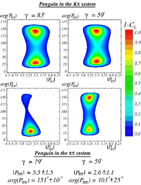
Figure -418: Confidence level plots for the complex parameter $A_{cc}^{K\pi}$ for $\gamma=83^{\circ}$ (left hand side) and $\gamma=59^{\circ}$ (right hand side). On the top we show the confidence levels without using $Br(\bar{B}^{0}\to\pi^{+}K^{-})$, while the bottom plot includes this branching ratio. We also show the value of $P_{\pi\pi}$, which is idential to the $P_{K\pi}$ in the SU(3) limit.

IV.4.4 Predictions for other $K\pi$ and $K\bar{K}$ observables

Using the hadronic parameters extracted from the $B\to\pi\pi$ decays ($\zeta^{B\pi}$, $\zeta_{J}^{B\pi}$ and $P_{\pi\pi}$), the value for $P_{K\pi}$ determined from the decays $B^{-}\to\pi^{-}\bar{K}^{0}$ and $\bar{B}^{0}\to\pi^{-}K^{+}$ decays and independently varying $\zeta^{BK}+\zeta^{BK}_{J}=0.2\pm 0.1$ and $\beta_{\pi}\zeta^{BK}_{J}=0.10\pm 0.05$, we can calculate all the remaining currently measured $K\pi$ observables. The results are given in Table 4 for $\gamma=83^{\circ}$ and $\gamma=59^{\circ}$, respectively. We also show these results in Figs. -417 and -416. The data used in the fit are shown in red below the dashed dividing line while those above the line are predictions. Note that there is one more piece of data below the line than there are parameters.

In Fig. -417 we see that $\gamma=83^{\circ}$ gives a good match to the $B\to\pi\pi$ data except for the asymmetry $C(\pi^{0}\pi^{0})$. When taking into account the theoretical error the most striking disagreements are the ${\rm Br}(K^{-}\pi^{+})$ at $2.3\sigma$ and the CP-asymmetry $A_{\rm CP}(K^{-}\pi^{0})$ at $2.6\sigma$. All other predictions agree within the uncertainties. Note that one could demand that $A_{\rm CP}(K^{-}\pi^{0})$ be reproduced, which would imply a negative value of $\zeta_{J}^{BK}$ (a naive fit for $\gamma=83^{\circ}$ gives $\zeta_{J}^{BK}\sim-0.15$). Note however, that this would imply that both perturbation theory at the intermediate scale $\mu=\sqrt{E\Lambda}$ and SU(3) are badly broken.

The situation in Fig. -416 with $\gamma=59^{\circ}$ is similar except that the theoretical prediction for ${\rm Br}(\pi^{+}\pi^{0})$ moves somewhat. The ${\rm Br}(K^{-}\pi^{+})$ deviation is reduced to $1.6\sigma$ and asymmetry $A(K^{-}\pi^{0})$ is still $2.6\sigma$. All other predictions agree within the uncertainties.

	Expt.	Theory	Theory
		($\gamma=83^{\circ}$)	($\gamma=59^{\circ}$)
Data in Fit
$S({\pi^{+}\pi^{-}})$	$-0.50\pm 0.12$	$-0.50\pm 0.10$	$-0.51\pm 0.10$
$C({\pi^{+}\pi^{-}})$	$-0.37\pm 0.10$	$-0.37\pm 0.07$	$-0.38\pm 0.07$
${\rm Br}(\pi^{+}\pi^{-})$	$5.0\pm 0.4$	$5.0\pm 2.0$	$4.6\pm 1.8$
${\rm Br}(\pi^{+}\pi^{0})$	$5.5\pm 0.6$	$5.5\pm 2.2$	$7.3\pm 2.9$
${\rm Br}(\pi^{0}\pi^{0})$	$1.45\pm 0.29$	$1.45\pm 0.58$	$1.32\pm 0.53$
${\rm Br}(\bar{K}^{0}\pi^{-})$	$24.1\pm 1.3$	$24.1\pm 1.2$	$24.1\pm 1.2$
$A({{K}^{-}\!\pi^{+}})$	$-0.115\pm 0.018$	$-0.115\pm 0.023$	$-0.115\pm 0.023$
${\rm Br}(\bar{K}^{0}K^{-})$	$1.2\pm 0.3$	$1.2\pm 0.5$	$1.2\pm 0.5$
Predictions
$A({\pi^{+}\pi^{0}})$	$0.01\pm 0.06$	$\lesssim 0.05$	$\lesssim 0.05$
$A({\pi^{0}\pi^{0}})$	$0.28\pm 0.40$	$-0.48\pm 0.19$	$-0.52\pm 0.27$
$S(\pi^{0}\pi^{0})$		$0.84\pm 0.23$	$-0.14\pm 0.22$
${\rm Br}(\pi^{0}\bar{K}^{0})$	$11.5\pm 1.0$	$10.4\pm 1.1$	$10.9\pm 1.2$
${\rm Br}(\pi^{+}{K}^{-})$	$18.9\pm 0.7$	$24.0\pm 2.1$	$22.5\pm 2.1$
${\rm Br}(\pi^{0}{K}^{-})$	$12.1\pm 0.8$	$14.3\pm 1.5$	$12.7\pm 1.4$
$S({\pi^{0}K_{S}})$	$0.31\pm 0.26$	$0.77\pm 0.16$	$0.76\pm 0.16$
$A({\pi^{0}\!{K}^{-}})$	$0.04\pm 0.04$	$-0.183\pm 0.075$	$-0.184\pm 0.076$
$A({\bar{K}^{0}\!\pi^{0}})$	$-0.02\pm 0.13$	$0.103\pm 0.058$	$0.083\pm 0.047$
$A({\pi^{-}\!\bar{K}^{0}})$	$-0.02\pm 0.04$	$<0.1$	$<0.1$
${\rm Br}(K^{0}\bar{K}^{0})$	$0.96\pm 0.25$	$1.1\pm 0.3$	$1.1\pm 0.3$
${\rm Br}(K^{+}\!K^{-})$	$0.06\pm 0.12$	$\lesssim 0.1$	$\lesssim 0.1$
$A(\bar{K}^{0}K^{-})$		$\lesssim 0.2$	$\lesssim 0.2$
$A(\bar{K}^{0}K^{0})$		$\lesssim 0.2$	$\lesssim 0.2$

Table 4: Comparison of LO predictions versus data as in Figs.3,4. ${\rm Br}$’s are in units of $10^{-6}$. The theory errors displayed for quantities used in the fit show the relative weight for these observables from power corrections, while those for predictions include parameter uncertainty from the fit as well as from power corrections. CP asymmetries that are not shown in the table are not determined at this order.

For $B\to K\bar{K}$ the amplitude parameters in SCET satisfy $A_{KK}=B_{KK}$ and $E_{KK}=PA_{KK}=EW_{KK}=0$, and we obtain the prediction

$${\rm Br}(B^{-}\to K^{-}\bar{K}^{0}) = {\rm Br}(\bar{B}^{0}\to K^{0}\bar{K}^{0})$$ (103)

which agrees well with the latest data, and the expectation that $A_{\rm CP}(B^{-}\to K^{-}\bar{K}^{0})$, $A_{\rm CP}(\bar{B}^{0}\to K^{0}\bar{K}^{0})$, and ${\rm Br}(\bar{B}^{0}\to K^{-}\bar{K}^{+})$ will be suppressed.

Unfortunately, without the use of SU(3) we do not have enough experimental information to determine the hadronic parameters required to predict the $B\to K^{0}\bar{K}^{0}$ absolute branching ratio. It is however interesting to extract the penguin amplitude and compare with the other channels. We find

$$10^{3}|\hat{P}_{K\bar{K}}|=5.3\pm 0.8$$ (104)

Comparing with the penguin amplitudes extracted in $\pi\pi$ and in $K\pi$ we see that the combined SU(3) and SCET prediction, $P_{\pi\pi}\sim P_{K\pi}\sim P_{K\bar{K}}$, works quite well if $\gamma=83^{\circ}$.

V Conclusions

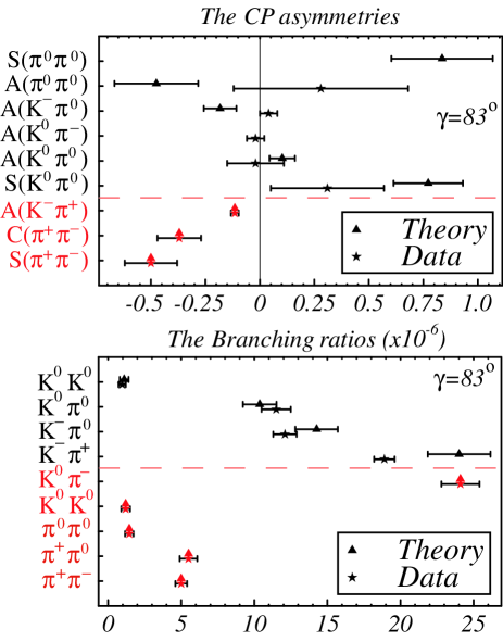
Figure -417: Comparison of theory and experiment for all available data in $B\to\pi\pi$ and $B\to K\pi$ decays, with $\gamma=83^{\circ}$. The 8 pieces of data in red (below the dashed line) have been used to determine the SCET hadronic parameters $\zeta^{B\pi}$, $\zeta_{J}^{B\pi}$, $P_{\pi\pi}$, $P_{K\pi}$ and $|P_{K}K|$, with $\zeta^{BK}$ and $\zeta_{J}^{BK}$ fixed as described in the text. The data above the line are predictions. The CP asymmetry in $B^{-}\to K^{0}\pi^{-}$ is expected to be small, but its numerical value is not predicted reliably.

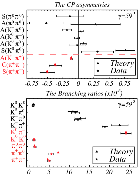
Figure -416: Same as Fig.3, but with $\gamma=59^{\circ}$.

Decays of $B$ mesons to two pseudoscalar mesons provide a rich environment to test our understanding of the standard model and to look for physics beyond the standard model. The underlying electroweak physics mediating these decays are contained in the Wilson coefficients of the electroweak Hamiltonian as well as CKM matrix elements. In order to test cleanly the standard model predictions for these short distance parameters, one requires a good understanding of the QCD matrix elements of the effective operators, which can not be calculated perturbatively.

At the present time, there are 5 well measured (with $<100\%$ uncertainty) observables in $B\to\pi\pi$, 5 in $B\to K\pi$ and 2 in $B\to KK$. Using only isospin symmetry (with corrections suppressed by $m_{u,d}/\Lambda$), the number of hadronic parameters required to describe these decays is 7, 11 and 11, respectively. The number of hadronic parameters can be reduced by two in the $\pi\pi$ system, if one drops the two operators $O_{7}$ and $O_{8}$, which have small Wilson coefficients in the standard model. If one is willing to take SU(3) (an expansion in $m_{s}/\Lambda$) as a good symmetry of QCD, the combined $B\to\pi\pi/K\pi$ system is described by 15 parameters, while the $B\to KK$ system adds another 4 parameters. Neglecting $O_{7}$ and $O_{8}$ with SU(3) reduces the number of parameters in the $\pi\pi/K\pi/K\bar{K}$ system to 15. Thus, at the present time there are more hadronic parameters than there are well measured observables.

In this paper we have studied these decays in a model independent way using SCET. This analysis exploits that the hadronic scale $\Lambda$ in QCD is much smaller than both in the large mass of the heavy quark and the large energy of the two light mesons. It follows that at leading order in the power expansion in $\Lambda_{\rm QCD}/Q$, where $Q\sim m_{b},E$, and using SU(2), there are four hadronic parameters describing $B\to\pi\pi$, five additional parameters describing $B\to K\pi$ and three additional parameters describing $B\to KK$. In the limit of exact SU(3) the four parameters describing $B\to\pi\pi$ are enough to describe all of these $B\to PP$ decays in SCET.

In SCET the electroweak penguin operators $O_{7,8}$ can be included without adding additional hadronic parameters. One can use the 5 pieces of well measured $\pi\pi$ data to determine the four hadronic parameters and the weak angle $\gamma$ gammafit , and with the current data one finds $\gamma=83^{\circ}\pm 8^{\circ}\pm 2^{\circ}$. This is still consistent with the direct measurement of this angle from $B\to DK$ HFAG , but is currently in conflict with the value of $\gamma$ from a global fit of the unitarity triangle at the $2\sigma$ level. It is too early to tell if this implies larger than expected power corrections in SCET or might be a first hint at new physics. When we proceed to analyze the decays $B\to K\pi$, we thus perform our analysis both for $\gamma=83^{\circ}$ and $\gamma=59^{\circ}$. For both of these values the direct CP asymmetry in $B\to\pi^{0}\pi^{0}$ is predicted to have the opposite sign from the measured value, but is still consistent at the $2\sigma$ level.

Moving on to $B\to K\pi$ decays, we analyzed the uncertainty in the Lipkin sum rule Lipkin for branching fractions and the CP-sum rule CPsum for rescaled CP-asymmetries as defined in Eqs. (72,73), giving our result in Eqs. (85,86). The CP-sum rule was found to be particularly accurate due to a suppression by three small parameters in SCET. The Lipkin sum rule is second order in small parameters and has a theoretical precision that also makes it an interesting observable. We conclude that both the Lipkin and CP-sum rules will provide very robust methods for testing the $K\pi$ data as the experimental errors decrease in the future.

Using the expectation that the hadronic parameters $\zeta^{BM}$ and $\zeta_{J}^{BM}$ in the factorization theorem are positive, we showed that the rescaled asymmetry $\Delta_{1}(\pi^{0}K^{-})$ should have the same sign and larger magnitude than the rescaled asymmetry $\Delta_{2}(\pi^{-}K^{+})$ which is well measured. This prediction is in conflict with the current data by $\sim 2\sigma$. Other sign and magnitude predictions are discussed in section IV.4.2.

The SCET amplitude formulas predict that in addition to the $\pi\pi$ parameters already determined, only the complex $K\pi$ penguin amplitude is required to describe the decays $B^{-}\to\pi^{-}\bar{K}^{0}$ and $B\to\pi^{+}K^{-}$. This happens because they involve $\zeta^{B\pi}$ and $\zeta_{J}^{B\pi}$, but do not involve $\zeta^{B\bar{K}}$ or $\zeta^{B\bar{K}}_{J}$. The well know prediction of a small CP asymmetry for $B^{-}\to\pi^{-}\bar{K}^{0}$ is reproduced in SCET. The large difference in ${\rm Br}(B\to\pi^{+}K^{-})$ and ${\rm Br}(B^{-}\to\pi^{-}\bar{K}^{0})$ is difficult to explain in the standard model with SCET. The $\gamma=59^{\circ}$ solution is not preferred by the combined SU(3)+SCET limit which predicts $P_{K\pi}\simeq P_{\pi\pi}$. These amplitudes agree well for $\gamma=83^{\circ}$.

Given the current uncertainties in the data, the remaining two hadronic parameters $\zeta^{BK}$ and $\zeta_{J}^{BK}$ can not yet be determined reliably. This also means that predictions for the remaining rates do not depend too sensitively on these parameters. Fixing their values to be close to those preferred by SU(3), but with 50% uncertainty, we obtained predictions for the remaining observables in Figures -417 and -416.

Finally, the decays $B\to KK$ require two additional hadronic parameters, which can only be determined once better data for both rates and CP asymmetries become available for these decays. One prediction of SCET, namely that ${\rm Br}(B\to K^{0}\bar{K}^{0})={\rm Br}(B^{-}\to K^{-}\bar{K}^{0})$ is well satisfied by the current data. In the SU(3) limit one expects that $P_{K\pi}\sim P_{K\bar{K}}$, and this result is in good agreement with the data.

In conclusion, several predictions of SCET work rather well, while for others there are discrepancies with the current data. It is too early to tell if the disagreements between theory and data are due to statistical fluctuations, to larger than expected power corrections or if they reveal a first glimpse of physics beyond the standard model. To answer this question, the experimental uncertainties need to be reduced and the convergence of the SCET expansion of QCD for nonleptonic decays has to be tested further both with nonleptonic and with semileptonic data agrs ; Hillf .

Appendix A Operators and Matrix Elements in SCET

At the scale $\mu\simeq m_{b}$ the Hamiltonian in Eq. (5) is matched onto operators in SCET. For the first two orders in the power expansion

$$H_{W}\!\! = \!\!\frac{2G_{F}}{\sqrt{2}}\sum_{n,{\bar{n}}}\bigg{\{}\sum_{i}\int[d\omega_{j}]_{j=1}^{3}c_{i}^{(f)}(\omega_{j})Q_{if}^{(0)}(\omega_{j})$$

$$+\sum_{i}\int[d\omega_{j}]_{j=1}^{4}b^{(f)}_{i}(\omega_{j})Q_{if}^{(1)}(\omega_{j})+{\cal Q}_{c\bar{c}}+\ldots\bigg{\}}\,,$$ (105)

The Wilson coefficients $c_{i}$ and $b_{i}$ are the Wilson coefficients that appear in Eqs. (III.1–36). The operators for the $\Delta S=0$ transitions are pipiChay ; bprs

$$Q_{1d}^{(0)} = \big{[}\bar{u}_{n,\omega_{1}}\bar{n}\!\!\!/P_{L}b_{v}\big{]}\big{[}\bar{d}_{{\bar{n}},\omega_{2}}n\!\!\!/P_{L}u_{{\bar{n}},\omega_{3}}\big{]}\,,$$ (106)

$$Q_{2d,3d}^{(0)} = \big{[}\bar{d}_{n,\omega_{1}}\bar{n}\!\!\!/P_{L}b_{v}\big{]}\big{[}\bar{u}_{{\bar{n}},\omega_{2}}n\!\!\!/P_{L,R}u_{{\bar{n}},\omega_{3}}\big{]}\,,$$

$$Q_{4d}^{(0)} = \big{[}\bar{q}_{n,\omega_{1}}\bar{n}\!\!\!/P_{L}b_{v}\big{]}\big{[}\bar{d}_{{\bar{n}},\omega_{2}}n\!\!\!/P_{L}\,q_{{\bar{n}},\omega_{3}}\big{]}\,,$$

$$Q_{5d,6d}^{(0)} = \big{[}\bar{d}_{n,\omega_{1}}\bar{n}\!\!\!/P_{L}b_{v}\big{]}\big{[}\bar{q}_{{\bar{n}},\omega_{2}}n\!\!\!/P_{L,R}q_{{\bar{n}},\omega_{3}}\big{]}\,,$$

and

$$Q_{1d}^{(1)}\!\! = \!\!\frac{-2}{m_{b}}\big{[}\bar{u}_{n,\omega_{1}}\,ig\,/\!\!\!\!{\cal B}^{\perp}_{n,\omega_{4}}P_{L}b_{v}\big{]}\big{[}\bar{d}_{{\bar{n}},\omega_{2}}n\!\!\!/P_{L}u_{{\bar{n}},\omega_{3}}\big{]}\,,$$

$$Q_{2d,3d}^{(1)} = \frac{-2}{m_{b}}\big{[}\bar{d}_{n,\omega_{1}}\,ig\,/\!\!\!\!{\cal B}^{\perp}_{n,\omega_{4}}P_{L}b_{v}\big{]}\big{[}\bar{u}_{{\bar{n}},\omega_{2}}n\!\!\!/P_{L,R}u_{{\bar{n}},\omega_{3}}\big{]}\,,$$

$$Q_{4d}^{(1)} = \frac{-2}{m_{b}}\big{[}\bar{q}_{n,\omega_{1}}\,ig\,/\!\!\!\!{\cal B}^{\perp}_{n,\omega_{4}}P_{L}b_{v}\big{]}\big{[}\bar{d}_{{\bar{n}},\omega_{2}}n\!\!\!/P_{L}\,q_{{\bar{n}},\omega_{3}}\big{]}\,,$$

$$Q_{5d,6d}^{(1)} = \frac{-2}{m_{b}}\big{[}\bar{d}_{n,\omega_{1}}\,ig\,/\!\!\!\!{\cal B}^{\perp}_{n,\omega_{4}}P_{L}b_{v}\big{]}\big{[}\bar{q}_{{\bar{n}},\omega_{2}}n\!\!\!/P_{L,R}q_{{\bar{n}},\omega_{3}}\big{]}\,,$$

$$Q_{7d}^{(1)}\!\! = \!\!\frac{-2}{m_{b}}\big{[}\bar{u}_{n,\omega_{1}}\,ig\,{\cal B}^{\perp\,\mu}_{n,\omega_{4}}P_{L}b_{v}\big{]}\big{[}\bar{d}_{{\bar{n}},\omega_{2}}n\!\!\!/\gamma^{\perp}_{\mu}P_{R}u_{{\bar{n}},\omega_{3}}\big{]}\,,$$

$$Q_{8d}^{(1)}\!\! = \!\!\frac{-2}{m_{b}}\big{[}\bar{q}_{n,\omega_{1}}\,ig\,{\cal B}^{\perp\,\mu}_{n,\omega_{4}}P_{L}b_{v}\big{]}\big{[}\bar{d}_{{\bar{n}},\omega_{2}}n\!\!\!/\gamma^{\perp}_{\mu}P_{R}q_{{\bar{n}},\omega_{3}}\big{]}\,.$$

The $\Delta S=1$ operators $Q_{is}^{(0)}$ are obtained by swapping $\bar{d}\to\bar{s}$. The “quark” fields with subscripts $n$ and ${\bar{n}}$ are products of collinear quark fields and Wilson lines with large momenta $\omega_{i}$. We have defined

$$\bar{u}_{n,\omega} =[\bar{\xi}_{n}^{(u)}W_{n}\,\delta(\omega\!-\!{\bar{n}}\!\cdot\!{\cal P}^{\dagger})]\,,$$ (107)

$$ig\,{\cal B}^{\perp\,\mu}_{n,\omega} =\frac{1}{(-\omega)}\,\big{[}W^{\dagger}_{n}[i{\bar{n}}\!\cdot\!D_{c,n},iD^{\mu}_{n,\perp}]W_{n}\delta(\omega-\bar{\cal P}^{\dagger})\big{]}$$

where $\bar{\xi}_{n}^{(u)}$ creates a collinear up-quark moving along the $n$ direction, or annihilates an antiquark. The $b_{v}$ field is the standard HQET field. For a complete basis we also need operators with octet bilinears, $T^{A}\otimes T^{A}$, but their matrix elements vanish at LO. The operators $Q_{7d}^{(1)}$ and $Q_{8d}^{(1)}$ also do not contribute at LO bprs , see also Kagan .

The leading order factorization theorem in Eq. (32) is generated by time ordered products of both the operators $Q^{(0)}$ and $Q^{(1)}$ with insertions of a subleading Lagrangian. T-products with $Q^{(0)}$ contribute to terms with $\zeta^{BM}$ and T-products with $Q^{(1)}$ contribute to those with $\zeta_{J}^{BM}$. It is convenient to define

$$\tilde{Q}_{i}^{(0)} =\big{[}\bar{q}^{i}_{n,\omega_{1}}\bar{n}\!\!\!/P_{L}b_{v}\big{]}\,,$$ (108)

$$\tilde{Q}_{i}^{(1)} =\frac{-2}{m_{b}}\big{[}\bar{q}^{i}_{n,\omega_{1}}\,ig\,/\!\!\!\!{\cal B}^{\perp}_{n,\omega_{4}}P_{L}b_{v}\big{]}\,,$$

$$\tilde{Q}_{i}^{\bar{n}} =\bar{q}^{i}_{{\bar{n}},\omega_{2}}n\!\!\!/P_{L,R}q^{\prime i}_{{\bar{n}},\omega_{3}}\,.$$ (109)

In $\tilde{Q}_{i}^{(0,1)}$ the flavor of the $\bar{q}^{i}_{n,\omega_{1}}$ terms matches that of the first bilinear in Eq. (106). In $\tilde{Q}_{i}^{\bar{n}}$ the flavor of $\bar{q}^{i}$ and $q^{\prime i}$ match those in the second bilinear of Eq. (106), and we have $P_{R}$ for $i=3,6$ and $P_{L}$ otherwise. The contributions to $B\to M_{1}M_{2}$ at LO are all from $\tilde{Q}_{i}^{\bar{n}}$ times the time-ordered products

$$T_{1}^{i} =\!\mbox{\large$\int$}d^{4}y\,T\big{[}\tilde{Q}^{(0)}_{i}(0)\>i{\cal L}^{(1)}_{\xi_{n}q}(y)\big{]}$$

$$\ \ +\mbox{\large$\int$}d^{4}y\,d^{4}y^{\prime}\,T\big{[}\tilde{Q}^{(0)}_{i}(0)\>i{\cal L}^{(1)}_{\xi_{n}q}(y)\>i{\cal L}_{\xi_{n}\xi_{n}}^{(1)}\!(y^{\prime})\big{]}\!$$

$$\ \ +\mbox{\large$\int$}d^{4}y\,d^{4}y^{\prime}\,T\big{[}\tilde{Q}^{(0)}_{i}(0)\>i{\cal L}^{(1)}_{\xi_{n}q}(y)\>i{\cal L}_{cg}^{(1)}(y^{\prime})\}\big{]}$$

$$\ \ +\mbox{\large$\int$}d^{4}y\,T\big{[}\tilde{Q}_{i}^{(0)}(0),i{\cal L}^{(1,2)}_{\xi_{n}q}(y)\big{]},\$$

$$T_{2}^{i}(z) =\!\mbox{\large$\int$}d^{4}y\>T\big{[}\tilde{Q}_{i}^{(1)}(0),i{\cal L}^{(1)}_{\xi_{n}q}(y)\big{]},$$ (110)

where $z$ and $1-z$ are the momentum fractions carried by the collinear quark and gluon field in $\tilde{Q}_{i}^{(1)}$. Here $T_{1}$ and $T_{2}$ are exactly the same T-products that occur in the heavy-to-light form factors bps5 . In addition we have operators/T-products whose matrix elements give $A_{cc}$ (see the appendix of Ref. diff1 for further discussion of these contributions). Using the collinear gluon fields defined in Ref. bps6 the Lagrangians in Eq. (A) are

$${\cal L}_{\xi\xi}^{(1)} = \big{(}\bar{\xi}_{n}W\big{)}\,iD\!\!\!\!/^{\perp}_{us}\frac{1}{\bar{\cal P}}\big{(}W^{\dagger}iD\!\!\!\!/^{\perp}_{c}\frac{\bar{n}\!\!\!/}{2}\xi_{n}\big{)}+\mbox{h.c.}\,,$$ (111)

$${\cal L}^{(1)}_{\xi q} = \bar{\xi}_{n}\>\frac{1}{i{\bar{n}}\!\cdot\!D_{c}}\>ig\,B\!\!\!\!/_{\perp}^{c}Wq_{us}\mbox{ + h.c.}\,,$$

$${\cal L}^{(2)}_{\xi q} = \bar{\xi}_{n}\frac{\bar{n}\!\!\!/}{2}\frac{1}{i{\bar{n}}\!\cdot\!D_{c}}\>ig\,n\!\cdot\!M\,W\,q_{us}$$

$$+\bar{\xi}_{n}\frac{\bar{n}\!\!\!/}{2}iD\!\!\!\!/_{\perp}^{\,c}\frac{1}{(i{\bar{n}}\!\cdot\!D_{c})^{2}}\>ig\,B\!\!\!\!/_{\perp}^{c}W\>q_{us}\mbox{ + h.c.}\,,$$

$${\cal L}_{cg}^{(1)} = \frac{2}{g^{2}}\>{\rm tr}\Big{\{}\big{[}i{D}_{0}^{\mu},iD_{c}^{\perp\nu}\big{]}\big{[}i{D}_{0\mu},WiD_{us\,\nu}^{\perp}W^{\dagger}\big{]}\Big{\}}\,,$$

where $iD_{0}^{\mu}=i{\cal D}^{\mu}+gA_{n}^{\mu}$.

In this paper we only used this factorization at the scale $m_{b}$, so the hadronic paramaters are defined by matrix elements of $T_{1}$ and $T_{2}$ and the ${\bar{n}}$-collinear operator, namely

$$\langle M_{n}|T_{1}^{i}|B\rangle={\cal C}_{i}(B,M)\>m_{B}\>\zeta^{BM}\,,$$ (112)

$$\langle M_{n}|T_{2}^{i}(z)|B\rangle={\cal C}_{i}(B,M)\>m_{B}\>\zeta_{J}^{BM}(z)\,,$$

$$\langle M_{\bar{n}}|\tilde{Q}_{i}^{\bar{n}}|0\rangle={\cal C}_{i}^{\prime}(B,M)\>m_{B}\>f_{M}\>\phi_{M}(u)$$

where $u$ and $1-u$ are momentum fractions for the quark and antiquark ${\bar{n}}$-collinear fields. Here ${\cal C}^{i}(B,M)$ and ${\cal C}_{i}^{\prime}(B,M)$ are simple Clebsch-Gordan coefficients. Putting the pieces together we have

$$A =\langle M_{1}M_{2}|H_{W}|\bar{B}\rangle$$ (113)

$$=\frac{2G_{F}m_{B}^{2}}{\sqrt{2}}\sum_{i}{\cal C}_{i}(B,M_{1})\>{\cal C}_{i}^{\prime}(B,M_{2})\>f_{M_{2}}$$

$$\ \ \times\bigg{[}\int_{0}^{1}\!\!dudz\>b_{i}(u,z)\zeta_{J}^{BM_{1}}(z)\phi_{M_{2}}(u)$$

$$\qquad+\zeta^{BM_{1}}\int_{0}^{1}\!\!du\>c_{i}(u)\phi_{M_{2}}(u)\bigg{]}+(1\leftrightarrow 2)\,$$

$$+A_{c\bar{c}}^{M_{1}M_{2}}\,.$$

This result was used to obtain Eq. (III.1–36) where the relevant combinations of ${\cal C}^{i}\>{\cal C}^{\prime i}$ coefficients can be read off from Table I of Ref. bprs (and do not asssume isospin symmetry). Here $A_{c\bar{c}}^{M_{1}M_{2}}$ contains Clebsch Gordan coefficients if for example SU(2) is used to relate these parameters in different channels. For amplitudes with no penguin contribution we have $A_{c\bar{c}}^{M_{1}M_{2}}=0$.

Appendix B Relationship between our amplitude parameterization and graphical amplitudes

In this appendix we show the relationship between the amplitude parameters defined in Eqs. (13)-(II.3) and the graphical amplitudes defined in graphical1 ; graphical2 . These relations are useful, since one can immediately read off SU(3) relations between different amplitudes, since the graphical amplitudes are SU(3) invariant. Note that while the amplitude paramters on the right hand side of equations (B,B, B) have the same name for the different processes, $\pi\pi$, $K\pi$, and $K\bar{K}$, they are only equal in the SU(3) limit.

The relations for the amplitude parameters in $B\to\pi\pi$ are

$$\hat{T}_{\pi\pi} = T+P_{ut}+E+PA_{ut}+EW^{C}+\frac{EW^{A}}{2}-\frac{EW^{E}}{2}$$

$$-\frac{EW^{P}}{2}-\frac{EW^{PA}}{2}$$

$$\hat{C}_{\pi\pi} = C-P_{ut}-E-PA_{ut}+\frac{3EW^{T}}{2}+\frac{EW^{C}}{2}$$

$$+\frac{EW^{P}}{2}+\frac{EW^{PA}}{2}+\frac{EW^{E}}{2}-\frac{EW^{A}}{2}$$

$$\hat{P}_{\pi\pi} = P_{ct}+PA_{ct}+EW^{C}+\frac{EW^{A}}{2}-\frac{EW^{E}}{2}$$

$$-\frac{EW^{P}}{2}-\frac{EW^{PA}}{2}$$

$$\hat{EW}^{T}_{\pi\pi} = \frac{3}{2}(EW^{T}+EW^{C})\,.$$ (114)

The amplitude parameters for $B\to K\pi$ decays can be written in terms of graphical amplitudes as follows:

$$\hat{T}_{K\pi} = T+P_{ut}+EW^{C}-\frac{EW^{P}}{2}-\frac{EW^{E}}{2}$$

$$\hat{C}_{K\pi} = C-P_{ut}+\frac{3EW^{T}}{2}+\frac{EW^{C}}{2}$$

$$+\frac{EW^{P}}{2}+\frac{EW^{E}}{2}$$

$$\hat{P}_{K\pi} = P_{ct}+EW^{E}-\frac{EW^{C}}{2}-\frac{EW^{P}}{2}$$

$$\hat{A}_{K\pi} = P_{ut}+A+EW^{E}-\frac{EW^{P}}{2}-\frac{EW^{C}}{2}$$

$$\hat{EW}^{T}_{K\pi} = \frac{3}{2}(EW^{T}+EW^{C})$$

$$\hat{EW}^{C}_{K\pi} = \frac{3}{2}(EW^{C}-EW^{E})\,,$$ (115)

Finally,for $B\to KK$ decays we find

$$\hat{A}_{KK} = P_{ut}+A-\frac{EW^{C}}{2}+EW^{E}-\frac{EW^{P}}{2}$$

$$\hat{B}_{KK} = P_{ut}+PA_{ut}-\frac{EW^{C}}{2}-EW^{A}$$

$$\hat{E}_{KK} = -E-PA_{ut}-\frac{EW^{A}}{2}+\frac{EW^{PA}}{2}$$

$$\hat{P}_{KK} = P_{ct}-\frac{EW^{C}}{2}+EW^{E}-\frac{EW^{P}}{2}$$

$$\hat{PA}_{KK} = PA_{ct}+\frac{EW^{A}}{2}-\frac{EW^{PA}}{2}$$

$$\hat{EW}_{KK} = -\frac{3EW^{A}}{2}-\frac{3EW^{E}}{2}\,.$$ (116)

References

- (1)
- (2) C. W. Bauer, S. Fleming and M. E. Luke, Phys. Rev. D 63, 014006 (2001); C. W. Bauer, S. Fleming, D. Pirjol and I. W. Stewart, Phys. Rev. D 63, 114020 (2001); C. W. Bauer and I. W. Stewart, Phys. Lett. B 516, 134 (2001); Phys. Rev. D 65, 054022 (2002); C. W. Bauer, S. Fleming, D. Pirjol, I. Z. Rothstein and I. W. Stewart, Phys. Rev. D 66, 014017 (2002).
- (3) HFAG, http://www.slac.stanford.edu/xorg/hfag/
- (4) B. Aubert et al. [BABAR Collaboration], Phys. Rev. Lett. 94, 181802 (2005) [arXiv:hep-ex/0412037]; (B. Aubert etal), Babar-CONF-05/13 (LepPho05 contributed paper); B. Aubert et al. [BABAR Collaboration], Phys. Rev. D 71, (19??) [arXiv:hep-ex/0503011].
- (5) Y. Chao et al. [Belle Collaboration], Phys. Rev. D 69, 111102 (2004) [arXiv:hep-ex/0311061]; K. Abe et al. [Belle Collaboration], Phys. Rev. Lett. 94, 181803 (2005) [arXiv:hep-ex/0408101].
- (6) A. Bornheim et al. [CLEO Collaboration], Phys. Rev. D 68, 052002 (2003) [arXiv:hep-ex/0302026].
- (7) A. Warburton [CDF Collaboration], Int. J. Mod. Phys. A 20, 3554 (2005) [arXiv:hep-ex/0411079].
- (8) M. Gronau and D. London, Phys. Rev. Lett. 65, 3381 (1990).
- (9) Y. Grossman and H. R. Quinn, Phys. Rev. D 58, 017504 (1998); J. Charles, Phys. Rev. D 59, 054007 (1999); M. Gronau et al., Phys. Lett. B 514, 315 (2001); M. Pivk and F. R. Le Diberder, Eur. Phys. J. C 39, 397 (2005) [arXiv:hep-ph/0406263]. charl
- (10) S. Gardner, arXiv:hep-ph/9906269; M. Gronau and J. Zupan, Phys. Rev. D 71, 074017 (2005) [arXiv:hep-ph/0502139]; S. Gardner, Phys. Rev. D 72, 034015 (2005) [arXiv:hep-ph/0505071].
- (11) J. Charles et al. [CKMfitter], arXiv:hep-ph/0406184; [http://ckmfitter.in2p3.fr/]
- (12) A. J. Buras, R. Fleischer, S. Recksiegel and F. Schwab, Phys. Rev. Lett. 92, 101804 (2004); C. W. Chiang, M. Gronau, J. L. Rosner and D. A. Suprun, arXiv:hep-ph/0404073; A. Ali, E. Lunghi and A. Y. Parkhomenko, arXiv:hep-ph/0403275.
- (13) M. Bona et al. [UTfit Collaboration], arXiv:hep-ph/0509219; [http://utfit.roma1.infn.it/]
- (14) S. Baek, F. J. Botella, D. London and J. P. Silva, Phys. Rev. D 72, 036004 (2005) [arXiv:hep-ph/0506075];
- (15) R. Godang et al. [CLEO Collaboration], Phys. Rev. Lett. 80, 3456 (1998) [arXiv:hep-ex/9711010].
- (16) Y. D. Yang, R. Wang and G. R. Lu, arXiv:hep-ph/0509273; R. Arnowitt, B. Dutta, B. Hu and S. Oh, arXiv:hep-ph/0509233; K. Agashe, M. Papucci, G. Perez and D. Pirjol, arXiv:hep-ph/0509117. S. Baek, P. Hamel, D. London, A. Datta and D. A. Suprun, Phys. Rev. D 71, 057502 (2005) [arXiv:hep-ph/0412086]. Acta Phys. Polon. B 36, 2015 (2005) [arXiv:hep-ph/0410407];
- (17) C. W. Chiang, M. Gronau, J. L. Rosner and D. A. Suprun, Phys. Rev. D 70, 034020 (2004) [arXiv:hep-ph/0404073].
- (18) A. J. Buras, R. Fleischer, S. Recksiegel and F. Schwab, Nucl. Phys. B 697, 133 (2004) [arXiv:hep-ph/0402112].
- (19) Y. Y. Chang and H. n. Li, Phys. Rev. D 71, 014036 (2005) [arXiv:hep-ph/0410005].
- (20) D. Suprun, talk at CKM 2005, http://ckm2005.ucsd.edu/.
- (21) Y. L. Wu and Y. F. Zhou, arXiv:hep-ph/0503077.
- (22) A. Khodjamirian, T. Mannel and M. Melcher, Phys. Rev. D 68, 114007 (2003) [arXiv:hep-ph/0308297].
- (23) R. Fleischer and T. Mannel, Phys. Rev. D 57, 2752 (1998) [arXiv:hep-ph/9704423]; M. Neubert and J. L. Rosner, Phys. Rev. Lett. 81, 5076 (1998); A. J. Buras, R. Fleischer and T. Mannel, Nucl. Phys. B 533, 3 (1998) [arXiv:hep-ph/9711262]; M. Neubert, JHEP 9902, 014 (1999);
- (24) M. Gronau, D. Pirjol and T. M. Yan, Phys. Rev. D 60, 034021 (1999) [Erratum-ibid. D 69, 119901 (2004)].
- (25) A. J. Buras and R. Fleischer, Eur. Phys. J. C 11, 93 (1999).
- (26) M. Beneke, G. Buchalla, M. Neubert and C. T. Sachrajda, Phys. Rev. Lett. 83, 1914 (1999) [arXiv:hep-ph/9905312]; Nucl. Phys. B 591, 313 (2000) [arXiv:hep-ph/0006124]; M. Beneke, G. Buchalla, M. Neubert and C. T. Sachrajda, Nucl. Phys. B 606, 245 (2001) [arXiv:hep-ph/0104110]; M. Beneke and M. Neubert, Nucl. Phys. B 675, 333 (2003) [arXiv:hep-ph/0308039].
- (27) A. Szczepaniak, E. M. Henley and S. J. Brodsky, Phys. Lett. B 243, 287 (1990); M. J. Dugan and B. Grinstein, Phys. Lett. B 255, 583 (1991); H. D. Politzer and M. B. Wise, Phys. Lett. B 257, 399 (1991); M. Bander, D. Silverman and A. Soni, Phys. Rev. Lett. 43, 242 (1979).
- (28) C. W. Bauer, D. Pirjol and I. W. Stewart, Phys. Rev. Lett. 87, 201806 (2001) [arXiv:hep-ph/0107002].
- (29) S. Mantry, D. Pirjol and I. W. Stewart, Phys. Rev. D 68, 114009 (2003) [arXiv:hep-ph/0306254].
- (30) J. g. Chay and C. Kim, Phys. Rev. D 68, 071502 (2003) [arXiv:hep-ph/0301055]; Nucl. Phys. B 680, 302 (2004) [arXiv:hep-ph/0301262].
- (31) Y.Y. Keum et al, Phys. Lett. B 504, 6 (2001); Phys. Rev. D 63, 054008 (2001); C. D. Lu et al., Phys. Rev. D 63, 074009 (2001).
- (32) M. Ciuchini et al., Nucl. Phys. B 501, 271 (1997); Phys. Lett. B 515, 33 (2001); P. Colangelo et al., Z. Phys. C 45, 575 (1990).
- (33) C. W. Bauer, D. Pirjol, I. Z. Rothstein and I. W. Stewart, Phys. Rev. D 70, 054015 (2004) [arXiv:hep-ph/0401188].
- (34) T. Feldmann and T. Hurth, JHEP 0411, 037 (2004) [arXiv:hep-ph/0408188].
- (35) C. W. Bauer, D. Pirjol, I. Z. Rothstein and I. W. Stewart, arXiv:hep-ph/0502094.
- (36) M. Beneke, G. Buchalla, M. Neubert and C. T. Sachrajda, arXiv:hep-ph/0411171.
- (37) H. n. Li, S. Mishima and A. I. Sanda, arXiv:hep-ph/0508041.
- (38) C. N. Burrell and A. R. Williamson, arXiv:hep-ph/0504024.
- (39) G. Buchalla and A. S. Safir, arXiv:hep-ph/0406016.
- (40) A. L. Kagan, Phys. Lett. B 601, 151 (2004) [arXiv:hep-ph/0405134].
- (41) S. J. Lee and M. Neubert, arXiv:hep-ph/0509350.
- (42) A. E. Blechman, S. Mantry and I. W. Stewart, Phys. Lett. B 608, 77 (2005) [arXiv:hep-ph/0410312].
- (43) P. Ball and R. Zwicky, Phys. Rev. D 71, 014015 (2005) [arXiv:hep-ph/0406232].
- (44) J. Bijnens and A. Khodjamirian, Eur. Phys. J. C 26, 67 (2002) [arXiv:hep-ph/0206252].
- (45) A. Khodjamirian, T. Mannel and B. Melic, Phys. Lett. B 571, 75 (2003) [Phys. Lett. B 572, 171 (2003)] [arXiv:hep-ph/0304179]; A. Khodjamirian, T. Mannel, M. Melcher and B. Melic, arXiv:hep-ph/0509049.
- (46) C. W. Bauer, I. Z. Rothstein and I. W. Stewart, Phys. Rev. Lett. 94, 231802 (2005) [arXiv:hep-ph/0412120].
- (47) Y. Grossman, A. Hocker, Z. Ligeti and D. Pirjol, arXiv:hep-ph/0506228.
- (48) M. Gronau, O. F. Hernandez, D. London and J. L. Rosner, Phys. Rev. D 50, 4529 (1994); Phys. Rev. D 52, 6374 (1995);
- (49) C. W. Bauer and D. Pirjol, Phys. Lett. B 604, 183 (2004) [arXiv:hep-ph/0408161].
- (50) G. Buchalla, A.J. Buras and M.E. Lautenbacher, Rev. Mod. Phys. 68, 1125 (1996).
- (51) D. Zeppenfeld, Z. Phys. C 8, 77 (1981).
- (52) M. J. Savage and M. B. Wise, Phys. Rev. D 39, 3346 (1989) [Erratum-ibid. D 40, 3127 (1989)].
- (53) B. Grinstein and R. F. Lebed, Phys. Rev. D 53, 6344 (1996) [arXiv:hep-ph/9602218].
- (54) A. P. Bakulev, AIP Conf. Proc. 756, 342 (2005) [arXiv:hep-ph/0412248]. A. P. Bakulev, S. V. Mikhailov and N. G. Stefanis, FizikaB 13, 423 (2004) [arXiv:hep-ph/0311140]; Phys. Lett. B 578, 91 (2004) [arXiv:hep-ph/0303039].
- (55) M. Neubert and J. L. Rosner, Phys. Lett. B 441, 403 (1998) [arXiv:hep-ph/9808493].
- (56) H. J. Lipkin, Phys. Lett. B 445, 403 (1999) [arXiv:hep-ph/9810351].
- (57) M. Gronau and J. L. Rosner, Phys. Rev. D 59, 113002 (1999) [arXiv:hep-ph/9809384].
- (58) D. Atwood and A. Soni, Phys. Rev. D 58, 036005 (1998) [arXiv:hep-ph/9712287].
- (59) I. Stewart, talk at Lepton Photon 2005, http://lp2005.tsl.uu.se/ lp2005/.
- (60) M. Beneke and T. Feldmann, Nucl. Phys. B 592, 3 (2001) [arXiv:hep-ph/0008255]. C. W. Bauer, D. Pirjol and I. W. Stewart, Phys. Rev. D 67, 071502 (2003) [arXiv:hep-ph/0211069]; B. O. Lange and M. Neubert, Nucl. Phys. B 690, 249 (2004) [Erratum-ibid. B 723, 201 (2005)] [arXiv:hep-ph/0311345]; M. Beneke and T. Feldmann, Nucl. Phys. B 685, 249 (2004) [arXiv:hep-ph/0311335]; R. J. Hill, T. Becher, S. J. Lee and M. Neubert, JHEP 0407, 081 (2004) [arXiv:hep-ph/0404217]; M. Beneke and D. Yang, arXiv:hep-ph/0508250; D. Pirjol and I. W. Stewart, Phys. Rev. D 67, 094005 (2003) [Erratum-ibid. D 69, 019903 (2004)] [arXiv:hep-ph/0211251].
- (61) S. Eidelman et al. [Particle Data Group], Phys. Lett. B 592, 1 (2004).
- (62) CKM conference 2005, http://ckm2005.ucsd.edu/.
- (63) C. W. Bauer, Z. Ligeti, M. Luke, A. V. Manohar and M. Trott, Phys. Rev. D 70, 094017 (2004) [arXiv:hep-ph/0408002]; I. I. Bigi and N. Uraltsev, Phys. Lett. B 579, 340 (2004) [arXiv:hep-ph/0308165].
- (64) B. O. Lange, M. Neubert and G. Paz, arXiv:hep-ph/0504071.
- (65) M. Okamoto et al., [Fermilab/MILC], Nucl. Phys. Proc. Suppl. 140, 461 (2005) [arXiv:hep-lat/0409116]; J. Shigemitsu et al., [HPQCD], arXiv:hep-lat/0408019.
- (66) M. C. Arnesen, B. Grinstein, I. Z. Rothstein and I. W. Stewart, Phys. Rev. Lett. 95, 071802 (2005) [arXiv:hep-ph/0504209].
- (67) C. W. Bauer, D. Pirjol and I. W. Stewart, Phys. Rev. D 67, 071502 (2003) [arXiv:hep-ph/0211069].
- (68) C. W. Bauer, D. Pirjol, I. Z. Rothstein and I. W. Stewart, arXiv:hep-ph/0502094.
- (69) C. W. Bauer, D. Pirjol and I. W. Stewart, Phys. Rev. D 68, 034021 (2003) [arXiv:hep-ph/0303156].
- (70) M. Neubert, JHEP 9902, 014 (1999) [arXiv:hep-ph/9812396]; J. Matias, Phys. Lett. B 520, 131 (2001) [arXiv:hep-ph/0105103]; M. Gronau and J. L. Rosner, Phys. Rev. D 71, 074019 (2005) [arXiv:hep-ph/0503131]; M. Gronau, Phys. Lett. B 627, 82 (2005) [arXiv:hep-ph/0508047].
- (71) T. Becher and R. J. Hill, arXiv:hep-ph/0509090; R. J. Hill, arXiv:hep-ph/0505129.