Indirect Detection of Kaluza–Klein Dark Matter from Latticized Universal Dimensions

Tomas Hällgren and Tommy Ohlsson 

^,Department of Theoretical Physics, School of Engineering Sciences, Royal Institute of Technology (KTH) – AlbaNova University Center,

Roslagstullsbacken 11, 106 91  Stockholm, Sweden

Abstract

We consider Kaluza–Klein dark matter from latticized universal dimensions. We motivate and investigate two different lattice models, where the models differ in the choice of boundary conditions. The models reproduce relevant features of the continuum model for Kaluza–Klein dark matter. For the model with simple boundary conditions, this is the case even for a model with only a few lattice sites. We study the effects of the latticization on the differential flux of positrons from Kaluza–Klein dark matter annihilation in the galactic halo. We find that for different choices of the compactification radius, the differential positron flux rapidly converges to the continuum model results as a function of the number of lattice sites. In addition, we consider the prospects for upcoming space-based experiments such as PAMELA and AMS-02 to probe the latticization effect.

1 Introduction

Today, cosmological measurements by, e.g., the Wilkinson Microwave Anisotropy Probe (WMAP) [1, 2], the Two-Degree Field Galaxy Redshift Survey (2dFGRS) [3], and the Sloan Digital Sky Survey (SDSS) [4] indicate that the energy and matter in the Universe could be distributed such that approximately 73 % is “dark energy” (maybe due to the cosmological constant $\Lambda$ in Einstein’s field equations) and approximately 23 % is “dark matter”, which leaves around 4 % as ordinary luminous matter in terms of baryons such as protons and neutrons, i.e., baryonic matter.

Further evidence for the presence of dark matter comes from, e.g., galactic rotational curves [5, 6] and studies of the observed redshift-luminosity relation of type Ia supernovae [7, 8]. All these data consistently point towards approximately 23 % dark matter. However, the nature of the dark matter is still unknown. Nevertheless, several dark matter candidates exist. Ordinary matter could make up a fraction of the dark matter in the form of massive compact halo objects (MACHOs) [9, 10]. This could be, e.g., faint stars or stellar remnants such as black holes. However, the MACHOs can not make up all of the dark matter.

One of the most plausible candidates for dark matter is weakly interacting massive particles (WIMPs) [11, 12]. These are hypothetical non-baryonic particles with masses in the GeV-TeV range. They are electrically neutral and assumed to carry a conserved quantum number to ensure their stability. Within this category, the prime candidate is the lightest supersymmetric particle – typically the neutralino [13]. It is electrically neutral and stable due to the conservation of R-parity.

Recently, an interesting alternative dark matter candidate has been intensively studied in the literature, which is so-called Kaluza–Klein dark matter [14, 15]. In models with universal extra dimensions [16, 17] (for the first model with TeV sized extra dimensions, see [18]), in which all standard model particles can move, the first excited state or mode of the hypercharge gauge boson is an excellent candidate for dark matter. The prospects for both direct and indirect detection are generally good. In particular, for indirect detection, the prospects are better than for supersymmetric particles. This is because the Kaluza–Klein gauge boson is a vector particle, whereas the neutralino is a Majorana particle, and thus, has a helicity suppressed annihilation cross-section. Therefore, one could obtain an excess of positrons from Kaluza–Klein dark matter annihilation in the galactic halo [19, 20] (for neutralino dark matter detection with positrons, see also [21, 22]). This positron flux could, e.g., be detected in balloon-borne experiments such as HEAT [23] or future space-based experiments such as PAMELA [24] and AMS-02 [25, 26].

In general, a major disadvantage for models with extra spatial dimensions is that they have coupling constants with negative mass dimension and are therefore not renormalizable. Hence, these models can only be considered as effective models, valid up to some cutoff energy scale, where some more fundamental theory is expected to describe physics. The cutoff procedure leads after dimensional reduction to an effective four dimensional description, but without the full higher-dimensional gauge invariance. One possibility to remedy these problems is offered by deconstructed [27] or latticized [28] extra dimensions.

We will in this paper consider latticized extra dimensions. In these type of models, the fundamental high-energy theory is four dimensional with a replicated gauge symmetry of the form $G\times G\times\ldots\times G$, where $G$ is a gauge group. In addition, it contains a set of scalar fields, so-called link fields, which “link” the gauge groups. If the potential of the scalar fields is chosen in an appropriate way, then one can generate the physics of an extra dimension in the infra-red regime. This happens when the link fields acquire vacuum expectation values and spontaneously break the original symmetry down to a diagonal subgroup of the symmetry. The resulting low-energy model is a model with an extra dimension, where the extra dimension has been put on a lattice. Note that the model with deconstructed dimensions is structurally similar but replaces the link scalar fields with fermion condensates.

In this way, models with deconstructed or latticized extra dimensions can have similar benefits as models with continuum extra dimensions, but since they in contrast with the latter preserves manifest gauge invariance and sometimes are renormalizable quantum field theories, they have a better defined short distance behavior. This could be relevant to models for Kaluza–Klein dark matter, where corrections from physics above the ultra-violet cutoff energy scale could be crucial when determining the nature of the lightest Kaluza–Klein particle [17]. Radiative corrections to Kaluza–Klein masses have been calculated for latticized abelian [29] and non-abelian [30] gauge theories compactified on $M^{4}\times S^{1}$. So far, these calculations have not been applied to the case of latticized universal extra dimensions, where there should be additional contributions to Kaluza–Klein masses from the orbifold fixed points. In this paper, we will not consider radiative corrections, but instead consider the prospects for observing the latticized model already at tree-level.

More specifically, we will consider two lattice models for a universal extra dimension, where the models differ in the choice of boundary conditions. The models are designed to mimic in the infra-red regime the continuum theory for Kaluza–Klein dark matter. In the ultra-violet regime, the higher-dimensional theory is replaced with completely four dimensional dynamics. We study the effects of the latticization and whether one could probe these effects in future experiments such as PAMELA and AMS-02.

The paper is organized as follows. In Sec. 2, we describe the model for a latticized universal dimension with simple boundary conditions. Next, in Sec. 3, we study the flux of positrons coming from Kaluza–Klein dark matter annihilations in the galactic halo and the prospects for probing the latticization in upcoming space-based experiments. Then, in Sec. 4, we consider a lattice model with modified boundary conditions. Finally, in Sec. 5, we summarize our results and present our conclusions.

2 Latticized Universal Dimensions

In this section, we will follow closely the results of Refs. [32, 31].

The model we will consider is a field theory in four dimensions with a product gauge group $G=\Pi_{j=0}^{N}SU(3)_{j}\times SU(2)_{j}\times U(1)_{j}$. The model contains fermions and gauge bosons as well as a set of scalar link fields $Q_{j,j+1},\Phi_{j,j+1}$, and $\phi_{j,j+1}$, where $j=0,1,\ldots,N-1$. The link fields transform as bifundamentals under adjacent gauge groups.

When the link fields acquire vacuum expectation values (VEVs), i.e., $\langle Q_{j,j+1}\rangle=v_{3}\mathbbm{1}_{3}$, $\langle\Phi_{j,j+1}\rangle=v_{2}\mathbbm{1}_{2}$, and $\langle\phi_{j,j+1}\rangle=v_{1}/\sqrt{2}$, where $\mathbbm{1}_{n}$ is the $n\times n$ identity matrix, the product gauge group is spontaneously broken down to the diagonal subgroup $SU(3)\times SU(2)\times U(1)$, which we identify as the standard model (SM) gauge group. One can arrange the parameters of the scalar potential in such a way that the link fields become non-linear sigma model fields in the low-energy effective theory. The low-energy effective theory can then be identified with a transverse lattice gauge theory [33], where only the extra dimension has been latticized. Since we are interested in a model that mimics the continuum theory for Kaluza–Klein dark matter, we will consider a latticized version of an $S^{1}/\mathbb{Z}_{2}$ orbifold. This topology has in the continuum theory the advantages of generating chiral zeroth modes and of removing unwanted scalar degrees of freedom, in agreement with observations. Also, the orbifold topology imply a discrete symmetry – Kaluza–Klein parity, which ensures the stability of the lightest Kaluza–Klein particle, and thus, making it a viable dark matter candidate. We will find that the lattice model considered in this section reproduces the essential features of the continuum $S^{1}/\mathbb{Z}_{2}$ orbifold.

The action for this theory can be split as $S=S_{{\rm gauge}}+S_{{\rm fermion}}+S_{{\rm Higgs}}$. In what follows, we will neglect electroweak symmetry breaking effects and so we will not further consider the contribution from the Higgs sector.

2.1 Gauge Sector

We will take the action of the gauge sector to be [32]

$$S_{{\rm gauge}} = \int{\rm d}^{4}x\bigg{[}\sum_{j=0}^{N-1}\left(|D_{\mu}\phi_{j,j+1}|^{2}+{\rm Tr}|D_{\mu}\Phi_{j,j+1}|^{2}+{\rm Tr}|D_{\mu}Q_{j,j+1}|^{2}\right)$$ (1)

$$-V(\phi,\Phi,Q)+\sum_{j=0}^{N}\left(-\frac{1}{4}F_{j\mu\nu}F^{\mu\nu}_{j}-\frac{1}{4}F_{j\mu\nu}^{a}F^{\mu\nu a}_{j}-\frac{1}{4}F_{j\mu\nu}^{b}F^{\mu\nu b}_{j}\right)\bigg{]},$$

where $a=1,2,3$ and $b=1,2,\ldots,8$. Here $V(\phi,\Phi,Q)$ is a suitably chosen scalar potential. The $Q_{j,j+1}$ fields transform under $SU(3)_{j}\times SU(3)_{j+1}$ as $(\bar{{\bf 3}},{\bf 3})$, $\Phi_{j,j+1}$ transform under $SU(2)_{j}\times SU(2)_{j+1}$ as $({\bar{\bf 2}},{\bf 2})$, and $\phi_{j,j+1}$ are charged under $U(1)_{j}\times U(1)_{j+1}$ as $(-Y_{\phi},Y_{\phi})$. We will set $Y_{\phi}=1/3$.

The covariant derivatives act on the link fields as

$$D_{\mu}\phi_{j,j+1} =\left(\partial_{\mu}+{\rm i}\tilde{g}_{Y}\frac{Y_{\phi}}{2}A_{j\mu}-{\rm i}\tilde{g}_{Y}\frac{Y_{\phi}}{2}A_{(j+1)\mu}\right)\phi_{j,j+1},$$ (2)

$$D_{\mu}\Phi_{j,j+1} =(\partial_{\mu}+{\rm i}\tilde{g}A_{j\mu}^{a}T_{j}^{a}-{\rm i}\tilde{g}A_{(j+1)\mu}^{a}T_{j+1}^{a})\Phi_{j,j+1},$$ (3)

$$D_{\mu}Q_{j,j+1} =(\partial_{\mu}+{\rm i}\hat{g}A_{j\mu}^{b}T_{j}^{b}-{\rm i}\hat{g}A_{(j+1)\mu}^{b}T_{j+1}^{b})Q_{j,j+1}.$$ (4)

where $T_{j}^{a}\,(a=1,2,3)$ are the generators of $SU(2)_{j}$, $T_{j}^{b}\,(b=1,2,\ldots 8)$ are the generators of $SU(3)_{j}$, and $\tilde{g}_{Y}$, $\tilde{g}$, and $\hat{g}$ are the coupling constants of $U(1)_{j}$, $SU(2)_{j}$, and $SU(3)_{j}$, respectively. We have assumed discrete translational invariance by setting $\tilde{g}_{Yj}\equiv\tilde{g}_{Y}$, $\tilde{g}_{j}\equiv\tilde{g}$, and $\hat{g}_{j}\equiv\hat{g}$, for all $j$. When the link fields acquire VEVs, the kinetic terms for the link fields generate mass matrices for the gauge bosons. Thus, for the $U(1)$ gauge fields, we obtain the mass terms

$$\mathcal{L}_{{\rm mass}}=\frac{1}{8}\tilde{g}_{Y}^{2}v_{1}^{2}Y_{\phi}^{2}\sum_{j=0}^{N-1}(A_{j}-A_{j+1})^{2}.$$ (5)

Similarly, for the other gauge fields, we obtain the same kind of mass terms.

Explicitly, the $(N+1)\times(N+1)$ tridiagonal mass-squared matrix reads

$$M^{2}=\frac{1}{8}\tilde{g}_{Y}^{2}v_{1}^{2}Y_{\phi}^{2}\left(\begin{matrix}1&-1\\ -1&2&-1\\ &\ddots&\ddots&\ddots\\ &&-1&2&-1\\ &&&-1&1\end{matrix}\right),$$ (6)

which can be diagonalized by a change of basis

$$A_{j}=\sum_{n=0}^{N}a_{jn}\tilde{A}_{n},$$ (7)

where

$$a_{jn}=\left\{\begin{array}[]{ll}\sqrt{\frac{2}{N+1}}\cos\left(\frac{2j+1}{2}\gamma_{n}\right),&n\neq 0\\ \sqrt{\frac{1}{N+1}},&n=0\end{array}\right..$$ (8)

Here $\gamma_{n}=n\pi/(N+1)$. In this basis, we now obtain

$$\mathcal{L}_{{\rm mass}}=\frac{1}{2}\sum_{n=0}^{N}m_{n}^{2}\tilde{A_{n}}\tilde{A_{n}},$$ (9)

where

$$m_{n}^{2}=\tilde{g}_{Y}^{2}v_{1}^{2}Y_{\phi}^{2}\sin^{2}\left[\frac{n\pi}{2(N+1)}\right].$$ (10)

In the limit $n\ll N$, we find a linear Kaluza–Klein spectrum $m_{n}\simeq n/R$ provided that we make the identification $\pi\tilde{g}_{Y}v_{1}Y_{\phi}/[2(N+1)]=1/R$. It should be noted that when referring to $R$, we refer to the radius of the extra dimension, whereas some other authors with the same notation refer to the size of the extra dimension (i.e., $\pi R$ for an $S^{1}/\mathbb{Z}_{2}$ orbifold).

2.2 Fermionic Sector

2.2.1 Fermions

Next, we include a set of fermions $L^{\alpha}_{j}=(\nu^{\alpha}_{j},e^{\alpha}_{j})^{T}$ and $E^{\alpha}_{j}$, for $j=0,1,\ldots,N$ and $\alpha=e,\mu,\tau$ (from now on generational indices will be suppressed). Here $L_{j}$ transforms as ${\bf 2}$ under $SU(2)_{j}$ and as a singlet under $SU(2)_{i}$, for $i\neq j$. Furthermore, $L_{j}$ is charged under $U(1)_{j}$ as $Y_{d}=-1$. The field $E_{j}$ is a singlet under all $SU(2)$ groups and is charged under $U(1)_{j}$ as $Y_{s}=-2$. Both $L_{j}$ and $E_{j}$ transform trivially under all $SU(3)$ groups.

In Ref. [31], the latticized action for the quark sector was considered. We construct analogously the action for leptons as $S_{{\rm fermion}}=S_{d}+S_{s}$, where $S_{d}$ refers to the part containing the $SU(2)$ doublet fields and $S_{s}$ contains the $SU(2)$ singlet fields. Here $S_{d}$ is given by

$$S_{d} =\int{\rm d}^{4}x\,\left\{\sum_{j=0}^{N}\bar{L}_{j}{\rm i}\gamma^{\mu}D_{\mu}L_{j}-\sum_{j=0}^{N}\left[M_{f}{\bar{L}}_{jL}\left(\frac{\Phi^{\dagger}_{j,j+1}}{v_{2}}\frac{\phi_{j,j+1}^{3}}{(v_{1}/\sqrt{2})^{3}}L_{j+1,R}-L_{jR}\right)+{\rm h.c.}\right]\right\},$$

where $M_{f}$ is a mass parameter which will be used when matching to the continuum model. The covariant derivative is given by $D_{\mu}L_{j}=\left(\partial_{\mu}-{\rm i}\tilde{g}A^{a}_{j\mu}T_{j}^{a}-{\rm i}\tilde{g}_{Y}\frac{Y_{d}}{2}A_{j\mu}\right)L_{j}$. If the index of a field is out of bounds, then it is implicit that the field is zero. For the $SU(2)$ singlet fields, we have

$$S_{s}=\int{\rm d}^{4}x\,\left\{\sum_{j=0}^{N}{\bar{E}}_{j}{\rm i}\gamma^{\mu}D_{\mu}E_{j}+\sum_{j=0}^{N}\left[M_{f}{\bar{E}}_{jR}\left(\frac{\phi_{j,j+1}^{6}}{(v_{1}/\sqrt{2})^{6}}E_{j+1,L}-E_{jL}\right)+{\rm h.c.}\right]\right\},$$ (12)

where the covariant derivate is given by $D_{\mu}E_{j}=\left(\partial_{\mu}-{\rm i}\tilde{g}_{Y}\frac{Y_{s}}{2}A_{j\mu}\right)E_{j}$. Note that the signs for the mass terms in Eqs. (2.2.1) and (12) are different. This is a characteristic feature of theories with continuous universal extra dimensions after dimensional reduction [16]. Here, as in Ref. [34], it has been obtained by choosing different signs for the Wilson terms when deriving Eqs. (2.2.1) and (12). The signs for the mass terms are also in agreement with the corresponding results for the quark sector in Ref. [31].

In order to obtain chiral zeroth modes, we take the doublet fields to satisfy $L_{0R}=0$ and the singlet fields to satisfy $E_{0L}=0$. When the link fields acquire universal VEVs, we obtain mass matrices for the fermion fields. For example, in the doublet sector, we have

$$\mathcal{L}_{{\rm mass}}=-M_{f}\left[\bar{L}_{0L}L_{1R}+\sum_{j=1}^{N}{\bar{L}}_{jL}\left(L_{j+1,R}-L_{jR}\right)+{\rm h.c.}\right].$$ (13)

The corresponding mass matrix is diagonalized by a change of basis

$$L_{jL}=\sum_{n=0}^{N}a_{jn}\tilde{L}_{nL}\,,\quad\quad L_{jR}=\sum_{n=1}^{N}b_{jn}\tilde{L}_{nR}\,,$$ (14)

where the $a_{jn}$’s are given in Eq. (8) and

$$b_{jn}=\sqrt{\frac{2}{N+1}}\sin\left(j\gamma_{n}\right).$$ (15)

Thus, we obtain for the left-handed fields the masses

$$m_{n}^{2}=4M_{f}^{2}\sin^{2}\left[\frac{n\pi}{2(N+1)}\right],$$ (16)

where $n=0,1,\ldots,N$ and for the right-handed fields the same form for the masses, but now $n=1,2,\ldots,N$. Thus, there are no zeroth modes for the right-handed doublet fields. For $n\ll N$, we find a linear Kaluza–Klein spectrum if we make the identification $\pi M_{f}/(N+1)=1/R$. Note that with this identification the masses in Eq. (16) become identical to the masses in Eq. (10), after the corresponding identification of parameters has been made for Eq. (10). This is expected and it motivates the use of the same notation in Eqs. (10) and (16).

Similarly, we obtain a mass matrix for the singlet sector, which is diagonalized by a change of basis

$$E_{jL}=\sum_{n=1}^{N}b_{jn}\tilde{E}_{nL}\,,\quad\quad E_{jR}=\sum_{n=0}^{N}a_{jn}\tilde{E}_{nR}.$$ (17)

Note that $L_{jL}$ has the same expansion as $E_{jR}$, whereas $L_{jR}$ has the same expansion as $E_{jL}$. Furthermore, note that we obtain a right-handed zeroth mode and no left-handed zeroth modes for the singlet fields. This is because we have interchanged the role of the left- and right-handed fields in this case.

Note that, as in the continuum model, we obtain negative masses for the singlet fields. However, this can be remedied by a change of basis $\tilde{E}_{n}\rightarrow-\gamma_{5}\tilde{E}_{n}$, for $n=1,2,\ldots,N$ [16].

2.2.2 Fermion Gauge Boson Couplings

Now, we consider the couplings between fermions and the $U(1)$ gauge bosons. For the $SU(2)$ doublet fields, we obtain from the fermionic kinetic terms $\sum_{j=0}^{N}\bar{L}_{j}{\rm i}\gamma^{\mu}D_{\mu}L_{j}$, the couplings $\tilde{g}_{Y}\frac{Y_{d}}{2}\sum_{j=0}^{N}\bar{L}_{j}\gamma^{\mu}A_{j\mu}L_{j}$. In the mass eigenbasis, we have for the left-handed fields

$$\mathcal{L}_{ffA}=\tilde{g}_{Y}\frac{Y_{d}}{2}\sum_{n,m,l}\sum_{j}a_{jn}a_{jm}a_{jl}\bar{\tilde{L}}_{nL}\tilde{A}_{m\mu}\gamma^{\mu}\tilde{L}_{lL}.$$ (18)

Using the orthogonality relations given in Appendix A, we have

$$\mathcal{L}_{ffA}=\tilde{g}_{Y}\frac{Y_{d}}{2\sqrt{N+1}}\bar{\tilde{L}}_{1L}\tilde{A}_{1\mu}\gamma^{\mu}\tilde{L}_{0L}+{\rm h.c.}+\ldots,$$ (19)

where the dots indicate terms that are not directly relevant to our discussion. In the continuum model, the corresponding coupling is given by [35, 16]

$$\mathcal{L}_{{\rm cont.}}=\frac{1}{4}g_{Y}Y_{d}\bar{L}_{L}^{(1)}A_{\mu}^{(1)}\gamma^{\mu}(1-\gamma_{5})L^{(0)}+{\rm h.c.}.$$ (20)

There is an additional factor $1/2$ in Eq. (20) which is not present in Ref. [35]. This is simply due to the fact that we have chosen a different convention for the hypercharge assignment. If we identify $\tilde{g}_{Y}/\sqrt{N+1}=g_{Y}$, then we observe that we have the same coupling as for the continuum case.

For the singlet fields, we obtain from the kinetic terms $\sum_{j=0}^{N}\bar{E}_{j}{\rm i}\gamma^{\mu}D_{\mu}E_{j}$ the couplings $\tilde{g}_{Y}\frac{Y_{s}}{2}\sum_{j=0}^{N}\bar{E}_{j}\gamma^{\mu}A_{j\mu}E_{j}$. In the mass eigenbasis, we have for the right-handed fields

$$\mathcal{L}_{{ffA}}=\tilde{g}_{Y}\frac{Y_{s}}{2}\sum_{n,m,l}\sum_{j}a_{jn}a_{jm}a_{jl}\bar{\tilde{E}}_{nR}\tilde{A}_{m\mu}\gamma^{\mu}\tilde{E}_{lR}.$$ (21)

Again using the orthogonality relations, we have

$$\mathcal{L}_{ffA}=-\tilde{g}_{Y}\frac{Y_{s}}{2\sqrt{N+1}}\bar{\tilde{E}}_{1R}\tilde{A}_{1\mu}\gamma^{\mu}\tilde{E}_{0R}+{\rm h.c.}+\ldots,$$ (22)

where we have redefined the singlet fields $\tilde{E}_{n}\rightarrow-\gamma_{5}\tilde{E}_{n}$, for $n=1,2,\ldots,N$, in order to obtain positive masses in the singlet sector.

In the continuum model, the corresponding coupling in the singlet sector is [35, 16]

$$\mathcal{L}_{{\rm cont.}}=-\frac{1}{4}g_{Y}Y_{s}\bar{E}_{R}^{(1)}A_{\mu}^{(1)}\gamma^{\mu}(1+\gamma_{5})E^{(0)}+{\rm h.c.}$$ (23)

Thus, with the identification $\tilde{g}_{Y}/\sqrt{N+1}=g_{Y}$, we have the same coupling as for the continuum model.

3 Indirect Detection of Kaluza–Klein Dark Matter

In models of continuous universal extra dimensions, the annihilation of Kaluza–Klein gauge bosons can lead to an excess of positrons, which could be observed in balloon-borne and space-based experiments. The upcoming space-based experiments PAMELA and AMS-02 will reach considerably higher energies than the balloon-borne HEAT experiment did. The precision will also be largely improved. These improvements are due to the large acceptance and long exposure time of the new experiments. We focus in this paper on the PAMELA and AMS-02 experiments.

The space-based (or more specifically satellite-borne) PAMELA experiment is planned to be launched in June 2006. It has an acceptance of $20~{}{\rm cm}^{2}\,{\rm sr}$ and an exposure time of three years. The PAMELA experiment is optimized to measure the cosmic positron spectrum for positron energies up to 270 GeV.

The space-based AMS-02 experiment will be placed on the International Space Station and is planned to be launched in 2008. It has an acceptance of $450~{}{\rm cm}^{2}\,{\rm sr}$ and an exposure time of three years. The AMS-02 experiment is optimized to probe positron energies up to 400 GeV.

In this section, we consider the differential positron flux from Kaluza-Klein dark matter annihilations for the latticized model described in the previous sections. We examine the latticization effect and the prospects for upcoming experiments to probe this effect. It should be noted that Kaluza–Klein dark matter could also be observed indirectly by observing high-energy neutrinos or photons from dark matter annihilations or directly from scattering off nucleons [15, 36]. We leave the consideration of these cases for future work.

3.1 Annihilation of Gauge Bosons

Figure 1: Kaluza–Klein gauge boson annihilation into SM fermion pairs. Shown in the figure are the $t$- (left) and $u$-channel (right) diagrams.

Positrons can be produced from several annihilation channels. They can be produced both directly and indirectly through secondary decays. Here we will follow Ref. [15] and only consider positrons coming from direct $e^{+}e^{-}$ production. Positrons can also be produced from cascade decays of muons, taus, and heavy quarks. The lowest-order diagrams for the annihilation of the $U(1)$ gauge bosons to particle-antiparticle pairs are given in Fig. 1, where we will consider $f=e$, i.e., direct $e^{+}e^{-}$ production. Note that the fermionic propagators in Fig. 1 can be both left- and right-handed.

The analysis will be almost identical to that of the continuum case, we only have to replace the continuum Kaluza–Klein mode masses with the corresponding masses of the latticized model. Thus, from the Feynman rules in Fig. 7 in Appendix B, we obtain for the $t$-channel annihilation diagrams the amplitudes

$$\mathcal{M}_{L,R}=-{\rm i}g_{L,R}^{2}\bar{u}\gamma^{\mu}P_{L,R}\bigg{[}\frac{\left(k_{\rho}-p_{\rho}\right)\gamma^{\rho}}{(k-p)^{2}-m_{1}^{2}}\bigg{]}\gamma^{\nu}P_{L,R}v\epsilon_{\mu}\epsilon_{\nu}.$$ (24)

Here $u$ and $v$ denote four component spinors, $\epsilon_{\mu}$ and $\epsilon_{\nu}$ denote polarization vectors, and the parameters $g_{L,R}$ are given by

$$g_{L,R}=\frac{\tilde{g}_{Y}Y_{d,s}}{2\sqrt{N+1}}=\frac{g_{Y}Y_{d,s}}{2}.$$ (25)

For the $u$-channel diagrams, one obtains similar expressions. The cross-section for the continuum process has been calculated in Ref. [14]. In analogy with their result, we have

$$\sigma_{e^{+}e^{-}}=(g_{L}^{4}+g_{R}^{4})\frac{10(2m_{1}^{2}+s)\,{\rm artanh}(\beta)-7s\beta}{72\pi s^{2}\beta^{2}},$$ (26)

where

$$\beta=\sqrt{1-\frac{4m_{1}^{2}}{s}},$$ (27)

$m_{1}=2M_{f}\sin\left\{\pi/[2(N+1)]\right\}$ is the mass in the propagator, and $s=E_{CM}^{2}$ is a Mandelstam variable.

The differential positron flux is given by [37, 38]

$$\frac{{\rm d}\Phi_{e^{+}}}{{\rm d}\Omega{\rm d}E}=\frac{\rho_{0}^{2}}{m_{\tilde{A}_{1}}^{2}}\sum_{i}\sigma_{i}vB_{e^{+}}^{i}\int{\rm d}\epsilon f_{i}(\epsilon)G(\epsilon,E),$$ (28)

where the sum is over all annihilation channels, $\rho_{0}$ is the local dark matter density, and the $e^{+}$ branching fraction in channel $i$ is denoted by $B_{e^{+}}^{i}$. The mass $m_{\tilde{A}_{1}}=m_{1}$ is given by Eq. (10). The Green function $G(\epsilon,E)$ describes the propagation of the positrons through the galaxy and $f_{i}(\epsilon)$ denotes the initial positron energy distribution from channel $i$. As mentioned above, we will only consider the flux of positrons coming from direct $e^{+}e^{-}$ production. Thus, we will only be concerned with the cross section $\sigma_{e^{+}e^{-}}$. Since we are concerned with non-relativistic particles, we can make a series expansion of $\sigma_{e^{+}e^{-}}v$ for small velocities $v$. Thus, we obtain as in Ref. [15]

$$\sigma_{e^{+}e^{-}}v\simeq\frac{\tilde{g}_{Y}^{4}}{288\pi(N+1)^{2}m_{1}^{2}}\left(Y_{d}^{4}+Y_{s}^{4}\right).$$ (29)

Here we have written Eq. (29) explicitly in terms of the parameters of our original model. Recall that we have made the identification $\tilde{g}_{Y}/\sqrt{N+1}=g_{Y}$. Note also that this result includes a factor of 1/16, which is not present in Ref. [15]. This is because we have a different convention for the hypercharge assignment.

In calculating the differential positron flux, we have used the DarkSUSY package, see Refs. [39, 40]. In Figs. 2-6, we present the differential positron flux as a function of the positron energy for an inverse radius of 300 GeV, 450 GeV, 600 GeV, 750 GeV and 900 GeV respectively. We present the results for latticized models with $N=1$ (i.e., two lattice sites), $N=2$, and $N=3$. In addition, we give the continuum model results. We have chosen an isothermal sphere dark matter distribution with a halo size of $z_{h}=4\ {\rm kpc}$ and a local dark matter density of $\rho_{0}=0.3~{}{\rm GeV}\,{\rm cm}^{-3}$. The propagation parameters are taken from Ref. [41]. In Figs. 2-6, we also make a comparison with a model for the background differential positron flux. In all figures, we have chosen “model C” from Ref. [42]. We have included a factor 1/2 when calculating the differential positron flux, which comes from the fact that the gauge bosons always annihilate in pairs [43]. This factor has not always been accounted for in previous works, which is why our continuum results may differ by a factor 1/2 from some previous results on the continuum positron spectrum.

In Ref. [31], the bounds from electroweak precision observables on the mass $m_{1}$ of the first Kaluza–Klein mode for latticized and continuous universal extra dimensions are discussed. Note that for a continuous extra dimension $m_{1}$ equals the inverse radius $R^{-1}$, whereas for a latticized model we have that $m_{1}=2(N+1)(\pi R)^{-1}\sin\left\{\pi/[2(N+1)]\right\}$. In Ref. [31], the most stringent bound for a single continuous universal dimension was found to be $m_{1}=R^{-1}\gtrsim 400$ GeV ($95~{}\%$ CL). It was also found in Ref. [31] that the bound for a few-site lattice model can be lowered by 10 %-25 %, which would allow for a bound as low as $m_{1}\gtrsim 300$ GeV ($95~{}\%$ CL) for a few-site lattice model. The reason why the bounds are less restrictive for the lattice model is the realization of only a few Kaluza–Klein modes. This general feature of lattice models could be important for the PAMELA and AMS-02 experiments, which for a continuum model could be out of range of the acceptable energies. In a recent paper, Ref. [44], the authors argue that the bounds from electroweak precision observables could be improved, giving a bound as severe as $m_{1}=R^{-1}\gtrsim 700$ GeV ($99$ % CL). This bound was obtained by taking into account two-loop effects and LEP2 data. However, as argued above, the bounds for a lattice model should be less severe, especially for a few-site lattice model. There are also bounds from WMAP for the relic density of Kaluza–Klein dark matter [45]. It was found in Refs. [46, 47] that in the minimimal continuum UED model, including coannihilations, to account for the observed relic density, the ideal mass range for the lightest Kaluza–Klein particle should be $500$ GeV$-600$ GeV. Note that the bounds from WMAP can be lowered by assuming that Kaluza–Klein dark matter only makes up a fraction of the cold dark matter in the Universe. Of course, in this case, the annihilation rate in the halo will be reduced, making the detection of positrons with PAMELA and AMS-02 more difficult. In addition, there are bounds from direct detection [48], where the most stringent bound for a continuum model gives $m_{1}\gtrsim 400$ GeV [49], which is no more restrictive than the bounds from electroweak precision observables.

Note the peak in the positron spectrum at a positron energy equal to the WIMP mass (i.e., the mass of the first excited mode of the $U(1)$ gauge boson, $E_{e^{+}}=m_{\tilde{A}_{1}}=m_{1}$). This peak is due to the monoenergetic positron source and is a characteristic signature of Kaluza–Klein dark matter. In contrast, for neutralinos, the positron spectrum would be much smoother [50]. This is due to the Majorana nature of neutralinos, which leads to helicity suppression of direct $e^{+}e^{-}$ production. Note that since the lattice model only differ from the continuum model in the masses of the Kaluza–Klein modes, one could not by measuring the differential positron flux distinguish between a lattice model with a given radius and a continuum model with a larger radius, i.e., both models would make the same prediction. Such a degeneracy would also exist between a lattice model with parameters $N_{1}$ and $R_{1}$ and a different lattice model with parameters $N_{2}$ and $R_{2}$. Thus, one would require additional input from independent, different types of experiments in order to use the information from the differential positron flux to probe lattice effects.

We also observe that the lattice model converges very quickly to the continuum model. Given the uncertainties in astrophysical inputs and propagation models, it could be hard to detect such small deviations. For increasing values of $N$, the magnitude (i.e., the height of the peak) of the differential positron flux decreases and the peak is shifted towards the peak of the continuum model, whereas for decreasing values of the radius $R$ of the extra dimension, the separation among the peaks for different values of $N$ increases and the differential positron flux (as well as the height of the peak) decreases. This can be observed in Eq. (28), which shows that the decrease comes from the fact that the differential positron flux is suppressed by the mass of the Kaluza–Klein mode. Since the mass of the Kaluza–Klein mode is inversely proportional to the radius of the extra dimension, the flux will be smaller for a smaller radius, which can also be seen when comparing Figs. 2-6.

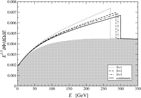
Figure 2: The differential positron flux (above background) for an inverse radius of 300 GeV as a function of positron energy, where we have only considered direct $e^{+}e^{-}$ production. In addition, positrons can also be produced from cascade decays of muons, taus and heavy quarks. Presented are latticized models with two lattice sites ($N=1$, dotted curve), three lattice sites ($N=2$, dashed curve) and four lattice sites ($N=3$, dash-dotted curve) as well as the continuum model (solid curve). Given is also an estimated background flux (gray shaded). The unit of the ordinate is cm^-2s^-1sr^-1GeV^2.5.

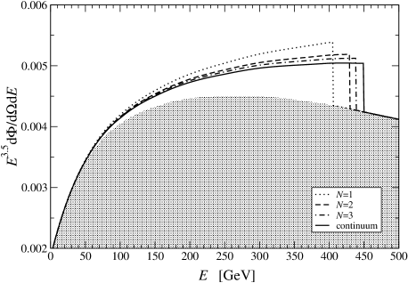
Figure 3: The differential positron flux (above background) for an inverse radius of 450 GeV as a function of positron energy, where we have only considered direct $e^{+}e^{-}$ production. In addition, positrons can also be produced from cascade decays of muons, taus and heavy quarks. Presented are latticized models with two lattice sites ($N=1$, dotted curve), three lattice sites ($N=2$, dashed curve) and four lattice sites ($N=3$, dash-dotted curve) as well as the continuum model (solid curve). Given is also an estimated background flux (gray shaded). The unit of the ordinate is cm^-2s^-1sr^-1GeV^2.5. For presentation purposes we have chosen the ordinate to start at $0.002$.

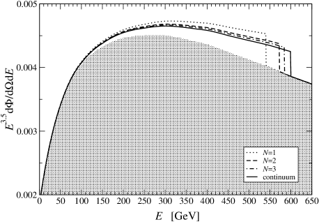
Figure 4: The differential positron flux (above background) for an inverse radius of 600 GeV as a function of positron energy, where we have only considered direct $e^{+}e^{-}$ production. In addition, positrons can also be produced from cascade decays of muons, taus and heavy quarks. Presented are latticized models with two lattice sites ($N=1$, dotted curve), three lattice sites ($N=2$, dashed curve) and four lattice sites ($N=3$, dash-dotted curve) as well as the continuum model (solid curve). Given is also an estimated background flux (gray shaded). The unit of the ordinate is cm^-2s^-1sr^-1GeV^2.5. For presentation purposes we have chosen the ordinate to start at $0.002$.

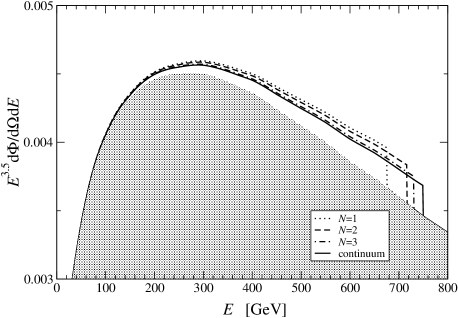
Figure 5: The differential positron flux (above background) for an inverse radius of 750 GeV as a function of positron energy, where we have only considered direct $e^{+}e^{-}$ production. In addition, positrons can also be produced from cascade decays of muons, taus and heavy quarks. Presented are latticized models with two lattice sites ($N=1$, dotted curve), three lattice sites ($N=2$, dashed curve) and four lattice sites ($N=3$, dash-dotted curve) as well as the continuum model (solid curve). Given is also an estimated background flux (gray shaded). The unit of the ordinate is cm^-2s^-1sr^-1GeV^2.5. For presentation purposes we have chosen the ordinate to start at $0.003$.

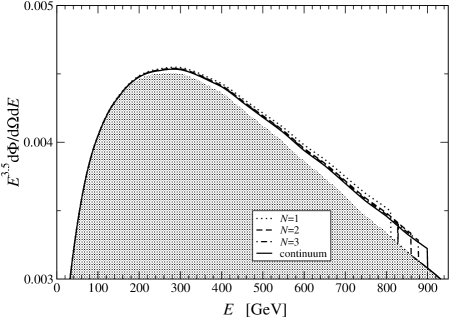
Figure 6: The differential positron flux (above background) for an inverse radius of 900 GeV as a function of positron energy, where we have only considered direct $e^{+}e^{-}$ production. In addition, positrons can also be produced from cascade decays of muons, taus and heavy quarks. Presented are latticized models with two lattice sites ($N=1$, dotted curve), three lattice sites ($N=2$, dashed curve) and four lattice sites ($N=3$, dash-dotted curve) as well as the continuum model (solid curve). Given is also an estimated background flux (gray shaded). The unit of the ordinate is cm^-2s^-1sr^-1GeV^2.5. For presentation purposes we have chosen the ordinate to start at $0.003$.

4 Modified Boundary Conditions

Finally, we will consider a model with more complicated boundary conditions. For the gauge fields, we impose that

$$A_{N}-A_{N-1}=0,$$ (30)

which is a discretized version of the continuum Neumann boundary condition. This will lead to the same type of gauge boson mass matrix as in Sec. 2, but now it will be an $N\times N$ matrix instead of an $(N+1)\times(N+1)$ matrix. Thus, the expansion in mass eigenstates will now take the form

$$A_{j}=\sum_{n=0}^{N-1}a_{jn}\tilde{A}_{n},$$ (31)

where the $a_{jn}$’s are defined as in Eq. (8), but with the replacement $N+1\rightarrow N$. The mass eigenvalues will now be $m_{n}^{2}=\tilde{g}_{Y}^{2}v_{1}^{2}Y_{\phi}^{2}\sin^{2}\left[n\pi/(2N)\right]$, where $n=0,1,\ldots N-1$. The correspondence with the continuum mass spectrum is obtained by requiring that $\pi\tilde{g}_{Y}v_{1}Y_{\phi}/(2N)=1/R$.

We impose as in Ref. [32] discretized Neumann boundary conditions in the fermionic sector by requiring that $L_{jL}$ and $E_{jR}$ satisfy

$$L_{NL}-L_{N-1,L}=0\quad\mbox{and}\quad E_{NR}-E_{N-1,R}=0.$$ (32)

We take the $L_{jR}$ and $E_{jL}$ fields to satisfy discretized Dirichlet boundary conditions, i.e., we impose that $L_{0R}=L_{NR}=0$ and $E_{0L}=E_{NL}=0$. In this way, we obtain, as in the continuum model, chiral zeroth modes. The corresponding mass matrix is diagonalized by a change of basis

$$L_{jL}=\sum_{n=0}^{N-1}a_{jn}\tilde{L}_{nL}\,,\quad\quad L_{jR}=\sum_{n=1}^{N-1}b_{jn}\tilde{L}_{nR}\,,$$ (33)

where the $a_{jn}$’s and $b_{jn}$’s are given in Eqs. (8) and (15), respectively, again with the replacement $N+1\rightarrow N$. We obtain for the left- and right-handed handed fields the masses $m_{n}^{2}=4M_{f}^{2}\sin^{2}\left[n\pi/(2N)\right]$. For $n\ll N$, we find a linear Kaluza–Klein spectrum by making the identification $\pi M_{f}/N=1/R$.

Similarly, we obtain a mass matrix for the singlet sector, which is diagonalized by a change of basis

$$E_{jL}=\sum_{n=1}^{N-1}b_{jn}\tilde{E}_{nL}\,,\quad\quad E_{jR}=\sum_{n=0}^{N-1}a_{jn}\tilde{E}_{nR}.$$ (34)

We obtain as in Sec. 2.2.1 negative masses for the singlet fields, which can be remedied by a change of basis $\tilde{E}_{n}\rightarrow-\gamma_{5}\tilde{E}_{n}$, for $n=1,2,\ldots,N-1$.

4.1 Fermion Gauge Boson Couplings

Analogously to Sec. 2.2.2, we derive in this section the couplings between fermion and gauge bosons for the model with modified boundary conditions. First, we consider the $SU(2)$ doublet fields and find for the left-handed fields the couplings

$$\mathcal{L}_{ffA} = \tilde{g}_{Y}\frac{Y_{d}}{2}\bigg{\{}\Delta_{0}\tilde{A}_{1\mu}\bar{\tilde{L}}_{0L}\gamma^{\mu}\tilde{L}_{0L}+\big{[}(\Delta_{1}+\sqrt{1/N})\tilde{A}_{1\mu}\bar{\tilde{L}}_{0L}\gamma^{\mu}\tilde{L}_{1L}+{\rm h.c.}\big{]}$$ (35)

$$+\sum_{l=2}^{N-1}\left(\Delta_{l}\tilde{A}_{1\mu}\bar{\tilde{L}}_{0L}\gamma^{\mu}\tilde{L}_{lL}+{\rm h.c.}\right)+\ldots\bigg{\}},$$

where again the dots indicate terms that are not directly relevant to our discussion and

$$\Delta_{k}=\frac{1}{\sqrt{N}}a_{N1}a_{Nk}=\left\{\begin{array}[]{ll}\frac{2}{\sqrt{N^{3}}}\cos\left(\frac{2N+1}{2}\gamma_{1}\right)\,\cos\left(\frac{2N+1}{2}\gamma_{k}\right),&k\neq 0\\ \\ \sqrt{\frac{2}{N^{3}}}\cos\left(\frac{2N+1}{2}\gamma_{1}\right),&k=0\end{array}\right..$$ (36)

For small or moderate $N$, the couplings in Eq. (35) deviate from the continuum results, see Eq. (20). The deviation is encoded in the parameters $\Delta_{k}$. Each of them goes as $1/N$, after one factor $1/\sqrt{N}$ has been absorbed in the redefinition of the coupling constant. Thus, for large number of lattice sites, the contribution from the $\Delta_{k}$ parameters become negligible and we reproduce the continuum results.

Second, in the singlet sector, we find the following couplings

$$\mathcal{L}_{ffA} = \tilde{g}_{Y}\frac{Y_{s}}{2}\bigg{\{}\Delta_{0}\tilde{A}_{1\mu}\bar{\tilde{E}}_{0R}\gamma^{\mu}\tilde{E}_{0R}-\big{[}(\Delta_{1}+\sqrt{1/N})\tilde{A}_{1\mu}\bar{\tilde{E}}_{0R}\gamma^{\mu}\tilde{E}_{1R}+{\rm h.c.}\big{]}$$ (37)

$$-\sum_{l=2}^{N-1}\left(\Delta_{l}\tilde{A}_{1\mu}\bar{\tilde{E}}_{0R}\gamma^{\mu}\tilde{E}_{lR}+{\rm h.c.}\right)+\ldots\bigg{\}},$$

where again we have redefined the singlet fields $\tilde{E}_{n}\rightarrow-\gamma_{5}\tilde{E}_{n}$, for $n=1,2,\ldots,N-1$, in order to obtain positive masses in the singlet sector. Precisely as for the doublet sector, the couplings in Eq. (37) deviate for small $N$ from the corresponding continuum couplings, see Eq. (23). However, in the large $N$ limit, we recover the continuum results.

Thus, we observe that for a small or moderate number of lattice sites, we obtain for the singlet and doublet sectors additional vertices, which are not present in the continuum. The Feynman rules for this model are given in Figs. 8 and 9 in Appendix B. The new Feynman rules will lead to additional diagrams for the annihilation process considered in Sec. 3.1. Thus, the positron flux will have a more complicated dependence on the latticization than in the model with the simpler boundary conditions, cf., Sec. 2. In particular, the degeneracy between the lattice model and a continuum model with larger radius is broken. However, we also observe that the analogue of Kaluza–Klein parity is explicitly broken. Note that Kaluza–Klein parity is necessary to ensure the stability of the lightest Kaluza–Klein mode, which is necessary for it to be a viable dark matter candidate. As the number of lattice sites is increased, Kaluza–Klein parity is approximately conserved. However, as we have seen, the lattice model converges very quickly to the continuum results and so in the region were Kaluza–Klein parity is approximately conserved, the deviance may anyway be too small to detect. Therefore, at this level, the model considered in this section is mostly of academic interest. A deeper analysis would be required to determine the phenomenological relevance of this model, but such an analysis is beyond the scope of this paper.

5 Summary and Conclusions

We have considered Kaluza–Klein dark matter from latticized universal dimensions. We have studied two different models for latticized universal dimensions, where the models differ in the choice of boundary conditions. We have examined to what extent the models can reproduce the continuum results for Kaluza–Klein dark matter. For the model with simple boundary conditions, we have found that we can reproduce the essential features of the continuum model, such as chiral zeroth modes and the relevant couplings, even for a few-site lattice model. We have especially examined the effects of the latticization on the differential positron flux from Kaluza–Klein dark matter annihilation and the prospects for upcoming experiments such as PAMELA and AMS-02 to probe the latticization effect. For the model with simple boundary conditions, we have found that the results would be equivalent to a continuum model with a larger radius. Thus, in conclusion, the results from such an experiment should be used in conjunction with the result from some different independent experiment in order to be able to probe lattice effects. We have also pointed out that, since the experimental bounds on latticized universal dimensions are less severe than for the corresponding continuum model, the prospects for detection for the lattice model are better. This could be important for the PAMELA and AMS-02 experiments, since these experiments could be out of range to detect the results of the continuum model.

For the model with modified boundary conditions, we have found a non-trivial dependence on the latticization. For a small number of lattice sites, Kaluza–Klein parity is violated, which means that, in this range, the model may not be a viable model for dark matter. For a large number of lattice sites, Kaluza–Klein parity is approximately conserved. However, due to the fast convergence to the continuum results, the prospects for detecting lattice effects in this range will be small.

Acknowledgments

We would like to thank Joakim Edsjö for help with DarkSUSY and Thomas Konstandin, Konstantin Matchev, Mark Pearce, and Gerhart Seidl for useful discussions.

This work was supported by the Royal Swedish Academy of Sciences (KVA), the Swedish Research Council (Vetenskapsrådet), Contract Nos. 621-2001-1611, 621-2002-3577, the Göran Gustafsson Foundation, and the Magnus Bergvall Foundation.

Appendix A Orthogonality Relations

In this appendix, we list some useful orthogonality relations for our formalism. In all of these relations, we have assumed that $0\leqslant n,m\leqslant N$. In the main text, when diagonalizing the mass matrices, we consider in Eq. (8) the expansion coefficients

$$a_{jn}=\left\{\begin{array}[]{ll}\sqrt{\frac{2}{N+1}}\cos\left(\frac{2j+1}{2}\gamma_{n}\right),&n\neq 0\\ \sqrt{\frac{1}{N+1}},&n=0\end{array}\right.,$$ (38)

where $\gamma_{n}=n\pi/(N+1)$. In addition, we have from Eq. (15) the expansion coefficients

$$b_{jn}=\sqrt{\frac{2}{N+1}}\sin\left(j\gamma_{n}\right).$$ (39)

Note that the expansion coefficients obey the following relations

$$\sum_{j=0}^{N}a_{jn}a_{jm}=\delta_{nm}\quad\mbox{and}\quad\sum_{j=0}^{N}b_{jn}b_{jm}=\delta_{nm}.$$ (40)

Thus, we have for $n,m,l\neq 0$ and $n,m,l\ll N$

$$\sum_{j=0}^{N}a_{jn}a_{jm}a_{jl}=\frac{1}{\sqrt{2(N+1)}}\left(\delta_{l,n+m}+\delta_{m,n+l}+\delta_{n,m+l}\right).$$ (41)

Note that if one of the indices $n$, $m$, and $l$ is zero, then we obtain

$$\sum_{j=0}^{N}a_{jn}a_{jm}a_{jl}=\frac{1}{\sqrt{N+1}}\left(\delta_{n0}\delta_{ml}+\delta_{m0}\delta_{nl}+\delta_{l0}\delta_{nm}\right).$$ (42)

Furthermore, if two are zero and one is non-zero, then we obtain zero. Finally, if all three of the indices $n$, $m$, and $l$ are zero, i.e., $(n,m,l)=(0,0,0)$, then we obtain

$$\sum_{j=0}^{N}a_{jn}a_{jm}a_{jl}=\frac{1}{\sqrt{N+1}}.$$ (43)

The corresponding relations for the $b_{jn}$’s will not be relevant for the purpose of this paper.

Appendix B Feynman Rules

In this appendix, we give the relevant Feynman rules for the models considered in the text. The Feynman rules are derived by first going to the mass eigenbasis and the simply reading off the rules for the vertices. In Fig. 7, we give the Feynman rules for the model considered in Sec. 2, and in Figs. 8 and 9, we give the Feynman rules for the model with modified boundary conditions considered in Sec. 4. Here $P_{R,L}=\frac{1}{2}(1\pm\gamma_{5})$ are the chirality projectors.

Figure 7: Feynman rules for the model with simple boundary conditions.

Figure 8: Feynman rules for the doublet sector of the model with modified boundary conditions.

Figure 9: Feynman rules for the singlet sector of the model with modified boundary conditions.

References

- [1] D. N. Spergel et al. (WMAP Collaboration), Astrophys. J. Suppl. 148, 175 (2003), astro-ph/0302209.
- [2] D. N. Spergel et al. (WMAP Collaboration), astro-ph/0603449
- [3] W. J. Percival et al. (2dFGRS Collaboration), Mon. Not. Roy. Astron. Soc. 337, 1068 (2002), astro-ph/0206256.
-
[4]
M. Tegmark et al.
(SDSS Collaboration), Phys. Rev.
D69, 103501
(2004),
astro-ph/0310723. - [5] M. Persic, P. Salucci, and F. Stel, Mon. Not. Roy. Astron. Soc. 281, 27 (1996), astro-ph/9506004.
-
[6]
Y. Sofue and
V. Rubin,
Ann. Rev. Astron. Astrophys.
39, 137 (2001),
astro-ph/0010594. - [7] R. A. Knop et al. (The Supernova Cosmology Project), Astrophys. J. 598, 102 (2003), astro-ph/0309368.
- [8] A. G. Riess et al. (The Supernova Search Team), Astrophys. J. 607, 665 (2004), astro-ph/0402512.
- [9] B. Paczynski, Astrophys. J. 304, 1 (1986).
- [10] J. Shaham and A. Dekel, Astron. Astrophys. 74, 186 (1979).
- [11] B. W. Lee and S. Weinberg, Phys. Rev. Lett. 39, 165 (1977).
- [12] J. E. Gunn, B. W. Lee, I. Lerche, D. N. Schramm, and G. Steigman, Astrophys. J. 223, 1015 (1978).
- [13] J. R. Ellis, J. S. Hagelin, D. V. Nanopoulos, K. A. Olive, and M. Srednicki, Nucl. Phys. B238, 453 (1984).
- [14] G. Servant and T. M. P. Tait, Nucl. Phys. B650, 391 (2003), hep-ph/0206071.
- [15] H.-C. Cheng, J. L. Feng, and K. T. Matchev, Phys. Rev. Lett. 89, 211301 (2002), hep-ph/0207125.
- [16] T. Appelquist, H.-C. Cheng, and B. A. Dobrescu, Phys. Rev. D64, 035002 (2001), hep-ph/0012100.
- [17] H.-C. Cheng, K. T. Matchev, and M. Schmaltz, Phys. Rev. D66, 036005 (2002), hep-ph/0204342.
- [18] I. Antoniadis, Phys. Lett. B246, 377 (1990).
- [19] D. Hooper and G. D. Kribs, Phys. Rev. D70, 115004 (2004), hep-ph/0406026.
- [20] D. Hooper and J Silk, Phys. Rev. D71, 083503 (2005), hep-ph/0409104.
- [21] M. Kamionkowski and M. S. Turner, Phys. Rev. D43, 1774 (1991).
- [22] E. A. Baltz and J. Edsjö, Phys. Rev. D59, 023511 (1999), astro-ph/9808243.
- [23] S. Coutu et al. (HEAT Collaboration), in *Hamburg 2001, Cosmic ray* (Copernicus Gesellschaft e.V., 2003), vol. 1 of ICRC 2001: Proceedings, pp. 1687–1690, prepared for 27th International Cosmic Ray Conference (ICRC 2001), Hamburg, Germany, August 7-15, 2001.
- [24] M. Boezio et al. (PAMELA Collaboration), Nucl. Phys. Proc. Suppl. 134, 39 (2004).
- [25] F. Barao (AMS-02 Collaboration), Nucl. Instrum. Meth. A535, 134 (2004).
- [26] C. Bosio (AMS-02 Collaboration), in *Tsukuba 2004, SUSY 2004*, edited by K. Hagiwara, J. Kanzaki, and N. Okada (KEK, 2004), vol. 2004-12 of KEK proceedings, pp. 701–704.
- [27] N. Arkani-Hamed, A. G. Cohen, and H. Georgi, Phys. Rev. Lett. 86, 4757 (2001), hep-th/0104005.
- [28] C. T. Hill, S. Pokorski, and J. Wang, Phys. Rev. D64, 105005 (2001), hep-th/0104035.
- [29] A. Falkowski, C. Grojean, and S. Pokorski, Phys. Lett. B581, 236–247 (2004), hep-ph/0310201
- [30] Z. Kunszt, A. Nyffeler, and M. Puchwein, JHEP 03, 061 (2004), hep-ph/0402269
- [31] J. F. Oliver, J. Papavassiliou, and A. Santamaria, Phys. Rev. D68, 096003 (2003), hep-ph/0306296.
- [32] H.-C. Cheng, C. T. Hill, S. Pokorski, and J. Wang, Phys. Rev. D64, 065007 (2001), hep-th/0104179.
- [33] W. A. Bardeen, R. B. Pearson, and E. Rabinovici, Phys. Rev. D21, 1037 (1980).
-
[34]
H.-C. Cheng,
C. T. Hill, and
J. Wang,
Phys. Rev. D64,
095003 (2001),
hep-ph/0105323. - [35] L. Bergström, T. Bringmann, M. Eriksson, and M. Gustafsson, JCAP 0504, 004 (2005), hep-ph/0412001.
- [36] L. Bergström, T. Bringmann, M. Eriksson, and M. Gustafsson, Phys. Rev. Lett. 94, 131301 (2005), astro-ph/0410359.
-
[37]
I. V. Moskalenko
and A. W.
Strong, Phys. Rev.
D60, 063003
(1999),
astro-ph/9905283. - [38] J. L. Feng, K. T. Matchev, and F. Wilczek, Phys. Rev. D63, 045024 (2001), astro-ph/0008115.
- [39] P. Gondolo, J. Edsjö, L. Bergström, P. Ullio, and E. A. Baltz, in *York 2000, The identification of dark matter*, edited by N. J. Spooner and V. Kudryavtsev (World Scientific, 2001), The Identification of Dark Matter: Proceedings, pp. 318–323, prepared for 3rd International Workshop on the Identification of Dark Matter (IDM2000), York, England, September 18-22, 2000, astro-ph/0012234.
- [40] P. Gondolo et al., JCAP 0407, 008 (2004), astro-ph/0406204.
- [41] J. Edsjö, M. Schelke, and P. Ullio, JCAP 0409, 004 (2004), astro-ph/0405414.
- [42] A. W. Strong, I. V. Moskalenko, and O. Reimer, Astrophys. J. 537, 763 (2000), astro-ph/9811296.
- [43] T. Bringmann, JCAP 0508, 006 (2005), astro-ph/0506219.
- [44] T. Flacke, D. Hooper, and J. March-Russell (2005), hep-ph/0509352.
- [45] C. L. Bennett et al., Astrophys.J.Suppl. 148, 1 (2003), astro-ph/0302207.
- [46] F. Burnell, and G. D. Kribs, Phys. Rev. D73, 015001 (2006), hep-ph/0509118.
- [47] K. Kong, and K. T. Matchev, JHEP 01, 038 (2006), hep-ph/0509119.
- [48] G. Servant, and T. M. P. Tait, New J. Phys. 4, 99 (2002), hep-ph/0209262.
- [49] V. Sanglard, (The EDELWEISS Collaboration) Phys. Rev. D71, 122002 (2005), astro-ph/0503265.
- [50] J. R. Ellis, J. L. Feng, A. Ferstl, K. T. Matchev, and K. A. Olive, Eur. Phys. J. C24, 311 (2002), astro-ph/0110225.