Soft Leptogenesis in Higgs Triplet Model

Abstract

We consider the minimal supersymmetric triplet seesaw model as the origin of neutrino masses and mixing as well as of the baryon asymmetry of the Universe, which is generated through soft leptogenesis employing a CP violating phase and a resonant behavior in the supersymmetry breaking sector. We calculate the full gauge–annihilation cross section for the Higgs triplets, including all relevant supersymmetric intermediate and final states, as well as coannihilations with the fermionic superpartners of the triplets. We find that these gauge annihilation processes strongly suppress the resulting lepton asymmetry. As a consequence of this, successful leptogenesis can occur only for a triplet mass at the TeV scale, where the contribution of soft supersymmetry breaking terms enhances the CP and lepton asymmetry. This opens up an interesting opportunity for testing the model in future colliders.

Leptogenesis is an elegant way to generate the baryon asymmetry of the Universe in connection with the origin of the observed neutrino masses and mixing through the seesaw mechanism fy . One way of understanding a tiny neutrino mass is to relate it with the small vacuum expectation value of a Higgs triplet Tss whose decay can also induce the cosmological baryon asymmetry in the presence of at least two Higgs triplets Tlepto or a right-handed neutrino hybrids as required by the generation of non-trivial CP and lepton asymmetry. In the minimal supersymmetric version with one pair of triplets, there is a new way of leptogenesis (called “soft leptogenesis”) in which CP phases in the soft terms can contribute to generate the lepton asymmetry softL ; kitano . Soft leptogenesis in the minimal supersymmetric Higgs triplet model has been considered first in Ref. softT .

In this paper, we revisit this last scenario to provide a careful analysis on the quantities for the lepton and CP asymmetries and their cosmological evolution by considering the full set of Boltzmann equations including thermal masses and the temperature supersymmetry breaking effects consistently. We will also derive a set of simple Boltzmann equations from the Maxwell-Boltzmann approximation taking into account the difference between the Bose–Einstein and Fermi–Dirac statistics, and show that they provide a fairly good approximation to the full Boltzmann equations.

The most important effect included in our analysis is the contribution of the gauge annihilation processes, which lead to a significant reduction of the resulting lepton asymmetry for the low Higgs triplet mass. The dynamics of such a system is analyzed in Ref. fry for the case of the conventional baryogenesis with heavy Higgs bosons in the $SU(5)$ unification scheme. Our analysis is extended to the lowest possible values of the Higgs triplet mass where, as will be shown in the following, the annihilation effect dominates over decays and inverse decays. Another crucial ingredient of soft leptogenesis is the suppression of the asymmetry due to a small difference between boson and fermion statistics at finite temperature. We find that this effect for low values of the triplet mass becomes subleading compared to that due to soft supersymmetry–breaking terms. Let us also note that the annihilation effect becomes irrelevant for a triplet mass higher than about $10^{10}$ GeV hambye05 , for which, however, the lepton asymmetry in the soft leptogenesis scenario is also suppressed, as it is inversely proportional to the triplet mass softL . As a result, we will conclude that the required baryon asymmetry can be generated only at the multi-TeV range of the Higgs triplet mass, and thus the model can lead to distinct collider signatures through, in particular, the production and decay of a doubly charged Higgs boson gunion ; chun03 . This opens up another interesting possibility for generating the neutrino masses and mixing as well as the cosmological baryon asymmetry at the TeV scale, which can be tested in future colliders tev ; apos .

In the supersymmetric form of the Higgs triplet model anna , one needs to introduce a vector-like pair of $\Delta=(\Delta^{++},\Delta^{+},\Delta^{0})$ and $\Delta^{c}=(\Delta^{c--},\Delta^{c-},\Delta^{c0})$ with hypercharge $Y=1$ and $-1$, allowing for the renormalizable superpotential as follows:

$$W=hLL\Delta+\lambda_{1}H_{1}H_{1}\Delta+\lambda_{2}H_{2}H_{2}\Delta^{c}+M\Delta\Delta^{c}$$ (1)

where $hLL\Delta$ contains the neutrino mass term, $h\nu\nu\Delta^{0}$. The soft supersymmetry breaking terms relevant for us are

$${-\cal L}_{soft} = \left\{hA_{L}LL\Delta+\lambda_{1}A_{1}H_{1}H_{1}\Delta\right.$$ (2)

$$+ \!\left.\lambda_{2}A_{2}H_{2}H_{2}\Delta^{c}+BM\Delta\Delta^{c}+h.c.\right\}$$

$$+ m_{\Delta}^{2}|\Delta|^{2}+m^{2}_{\Delta^{c}}|\Delta^{c}|^{2}.$$

Note that we have used the same capital letters to denote the superfields as well as their scalar components. We will consider the universal boundary condition of soft masses; $A_{L}=A_{1}=A_{2}=A$ and $m_{\Delta}=m_{\Delta^{c}}=m_{0}$. In the limit $M\gg m_{0},A$, the Higgs triplet vacuum expectation value $\langle\Delta^{0}\rangle=\lambda_{2}\langle H_{2}^{0}\rangle^{2}/M$ gives the neutrino mass

$$m_{\nu}=2h\lambda_{2}{v_{2}^{2}\over M}\,.$$ (3)

The mass matrix of the scalar triplets is diagonalized by

$$\Delta = {1\over\sqrt{2}}(\Delta_{+}+\Delta_{-})$$

$$\bar{\Delta}^{c} = {1\over\sqrt{2}}(\Delta_{+}-\Delta_{-})$$

where $\Delta_{\pm}$ are the mass eigenstates with the mass-squared values, $M^{2}_{\pm}=M^{2}+m_{0}^{2}\pm BM$, and the mass-squared difference, $\Delta M^{2}=2BM$. In terms of the mass eigenstates, the Lagrangian becomes

$${-\cal L} = {1\over\sqrt{2}}\Delta_{\pm}\big{[}h\,\tilde{L}\tilde{L}+h(A_{L}\pm M)\,LL$$

$$\lambda_{1}\,\tilde{H}_{1}\tilde{H}_{1}+\lambda_{1}(A_{1}\pm M)\,H_{1}H_{1}$$

$$\pm\lambda_{2}^{*}\,\bar{\tilde{H}}_{2}\bar{\tilde{H}}_{2}\pm\lambda_{2}^{*}(A_{2}^{*}\pm M)\,\bar{H}_{2}\bar{H}_{2}\big{]}+h.c.$$

The heavy particles $\bar{\Delta}_{\pm}$ decay to the leptonic final states, ${L}{L},\bar{\tilde{L}}\bar{\tilde{L}}$, as well as the Higgs final states, ${H}_{1}{H}_{1},{\tilde{H}}_{1}{\tilde{H}}_{1}$ and $\bar{H}_{2}\bar{H}_{2},\bar{\tilde{H}}_{2}\bar{\tilde{H}}_{2}$. Thus, the out-of-equilibrium decay $\bar{\Delta}_{\pm}\to{L}{L},\bar{\tilde{L}}\bar{\tilde{L}}$ can lead to lepton asymmetry of the universe.

In order to discuss how to generate a lepton asymmetry in the supersymmetric triplet seesaw model let us first consider the general case of a charged particle $X$ ($\bar{X}$) decaying to a final state $j$ ($\bar{j}$) and generating tiny CP asymmetric number densities, $n_{X}-n_{\bar{X}}$ and $n_{j}-n_{\bar{j}}$. The relevant Boltzmann equations in the approximation of Maxwell–Boltzmann distributions are

$${dY_{X}\over dz} = -zK\left[\gamma_{D}(Y_{X}-Y_{X}^{eq})+\gamma_{A}{(Y_{X}^{2}-Y_{X}^{eq\,2})\over Y_{X}^{eq}}\right]$$

$${dY_{x}\over dz} = -zK\gamma_{D}\left[Y_{x}-\sum_{k}2B_{k}{Y_{X}^{eq}\over Y_{k}^{eq}}Y_{k}\right]$$ (5)

$${dY_{j}\over dz} = 2zK\gamma_{D}\left[\epsilon_{j}(Y_{X}-Y_{X}^{eq})+B_{j}(Y_{x}-2{Y_{X}^{eq}\over Y_{j}^{eq}}Y_{j})\right]$$

where $Y$’s are the number densities in unit of the entropy density $s$ as defined by $Y_{X}\equiv n_{X}/s\approx n_{\bar{X}}/s$, $Y_{x}\equiv(n_{X}-n_{\bar{X}})/s$ and $Y_{j}\equiv(n_{j}-n_{\bar{j}})/s$. Here, the CP asymmetry $\epsilon_{j}$ in the decay $X\to j$ is defined by

$$\epsilon_{j}\equiv{\Gamma(X\to j)-\Gamma(\bar{X}\to\bar{j})\over\Gamma_{X}}.$$ (6)

In Eq. (Soft Leptogenesis in Higgs Triplet Model), $K\equiv\Gamma_{X}/H_{1}$ with the Hubble parameter $H_{1}=1.66\sqrt{g_{*}}M^{2}/m_{Pl}$ at the temperature $T=M$, and $B_{j}$ is the branching ratio of the decay $X\to j$. For the relativistic degrees of freedom in thermal equilibrium $g_{*}$, we will use the Supersymmetric Standard Model value: $g_{*}=228.75$.

The evolution of the $X$ abundance is determined by the decay and inverse decay processes, as well as by the annihilation effect described by the diagrams of FIG. 1, and are accounted for by the functions $\gamma_{D}$ and $\gamma_{A}$, respectively. Note that the triplets are charged under the Standard Model gauge group and thus have nontrivial gauge annihilation effect which turns out to be essential in determining the final lepton asymmetry. Moreover, as a consequence of unitarity, the relation $2Y_{x}+\sum_{j}Y_{j}\equiv 0$ holds, so that one can drop out the equation for $Y_{x}$, taking the replacement:

$$Y_{x}=-{1\over 2}\sum_{j}Y_{j}$$ (7)

in the last of Eqs. (Soft Leptogenesis in Higgs Triplet Model).

Figure 1: Diagrams contributing to the gauge–annihilation amplitude of triplet particles. $\tilde{\Delta}$, $\tilde{\Delta_{c}}$ represent the fermionic partners of $\Delta$ and $\Delta_{c}$, respectively, while $A$ indicates a gauge boson, $\lambda$ a gaugino, $h$ a Higgs particle, $\tilde{h}$ a higgsino, $f$ a fermion and $\tilde{f}$ a sfermion.

In our model, the heavy particle $X$ can be either of the six charged particles; $X=\Delta^{++}_{\pm},\Delta^{+}_{\pm}$ or $\Delta^{0}_{\pm}$. Each of them follows the first Boltzmann equation in Eq. (Soft Leptogenesis in Higgs Triplet Model) where $\gamma_{D}$ and $\gamma_{A}$ are given by

$$\gamma_{D} = {K_{1}(z)\over K_{2}(z)}$$ (8)

$$\gamma_{A} = {\alpha_{2}^{2}M\over\pi KH_{1}}\int^{\infty}_{1}\!\!dt\,\frac{K_{1}(2zt)}{K_{2}(z)}\,t^{2}\beta(t)\,\sigma(t)$$ (9)

with

$$\sigma(t)=(14+11t_{w}^{4})(3+\beta^{2})+(4+4t_{w}^{2}+t_{w}^{4})\left[16+4(-3-\beta^{2}+\frac{\beta^{4}+3}{2\beta}\ln\frac{1+\beta}{1-\beta})\right]$$

$$+4\left[-3+\left(4-\beta^{2}+\frac{(\beta^{2}-1)(2-\beta^{2})}{\beta}\ln\frac{1+\beta}{1-\beta}\right)\right],$$ (10)

where $t_{w}\equiv\tan(\theta_{W})$ with $\theta_{W}$ the Weinberg angle, and $\beta(t)\equiv\sqrt{1-t^{-2}}$. The function $\gamma_{D}$ is the ratio of the modified Bessel functions of the first and second kind which as usual takes into account the decay and inverse decay effects in the Maxwell–Boltzmann limit. The function $\gamma_{A}$ accounts for the annihilation cross-section of a triplet component $X$ summing all the annihilation processes; $X\bar{X}^{\prime}\to$ Standard Model gauge bosons/gauginos and fermions/sfermions where $X^{\prime}$ is some triplet component or its fermionic partner. The separate contribution of each diagram in FIG. 1 is detailed in the Appendix. As far as the Standard Model part is concerned, our result agrees with that of Ref. hambye05 , with one exception: the term proportional to $t_{w}^{2}$, due to the mixed gauge boson ($W_{3}B$) final state in diagrams (c–f) of FIG. 1, is missing in Ref. hambye05 . However, this difference concerns a subdominant contribution which is expected to have a negligible impact on phenomenology.

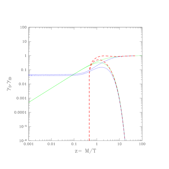
Figure 2: Decay and inverse-decay amplitudes entering in the Boltzmann equations. The solid lines show the decay amplitude $\gamma_{D}$ in the Maxwell–Bolzmann limit as given by Eq. (8), and the corresponding inverse–decay amplitude $\gamma_{ID}$. The dotted and dashed curves show the result of a full numerical evaluation of the same amplitudes for fermionic and bosonic final states, respectively.

The decay and inverse decay amplitudes in the Maxwell–Boltzmann limit are plotted in FIG. 2, along with a numerical evaluation of the same quantities in the case of bosonic and fermionic final states, where Bose–Einstein and Fermi–Dirac distributions, as well as thermal masses, are included in the calculation. We use this latter evaluation when we solve the full Boltzmann equations for the lepton asymmetry numerically. The last figure shows that the Boltzmann approximation is well justified as expected for the region of our relevance, $z>10$.

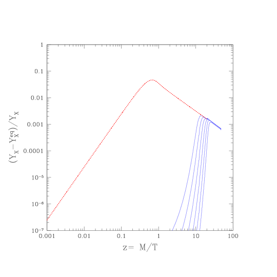
Figure 3: Fractional departure of the triplet comoving density $Y_{X}$ from its equilibrium value $Y^{eq}_{X}$, as a function of $z\equiv m/T$. The higher curve shows the result of a calculation where the gauge annihilation effect is neglected, while the lower ones show the same quantity including annihilation for $Im(A)$=1 TeV and $\log_{10}(M/{\rm GeV})=$ 8,7,6,5,4,3 from left to right. All curves are evaluated in the Maxwell–Boltzmann approximation.

Given $\gamma_{D}$ and $\gamma_{A}$, we can now analyze the thermal evolution of $Y_{X}$ fry . In FIG. 3, we plot the quantity $(Y_{X}-Y_{X}^{eq})/Y_{X}$, which quantifies the departure of the triplet density from its equilibrium value. In particular, the higher line shows the result when only the processes of decay and inverse decay to light particles are included in the calculation. As expected, since $K>>1$, $Y_{X}$ follows closely the equilibrium density $Y_{X}^{eq}$ with a slight deviation of order $10^{-1}$. However, annihilation is indeed important in our case and cannot be neglected. This is shown in the same figure by the lower curves, which represent the departure of the triplet density from its equilibrium value when annihilation is included. The importance of annihilation can be understood in the following way. The inverse decay freezes out at $z_{f}\approx 9$ for $K=32$ as $Kz_{f}^{5/2}e^{-z_{f}}=1$. On the other hand, the thermal averages of the annihilation and decay rate can be compared by considering the following ratio fry :

$${<\Gamma_{A}>\over<\Gamma_{D}>}(z_{f})\simeq 2{\alpha^{2}\over\alpha_{X}}z_{f}^{-3/2}e^{-z_{f}}\approx{2\times 10^{8}\mbox{ GeV}\over M},$$

where $\alpha_{X}=KH_{1}/M$. Thus, the annihilation effect becomes negligible for $M\lower 3.01385pt\hbox{$\;\stackrel{{\scriptstyle\textstyle>}}{{\sim}}\;$}10^{9}$ GeV. But in our case of soft leptogenesis, higher $M$ suppresses the lepton asymmetry as $\tilde{\epsilon}_{l}\propto A/M$, so there is a tension between these two effects, and lower values of $M$ turn out to be favored. In FIG. 3, one can see that, due to annihilation which freezes out at $z\approx 20$, $Y_{X}$ follows more closely its equilibrium density $Y_{X}^{eq}$ compared with the previous case, with a deviation which is now of order $10^{-3}$. In particular, this implies that the approximation

$$Y_{X}-Y_{X}^{eq}={-Y_{X}^{eq\prime}\over zK(\gamma_{D}+2\gamma_{A})}$$ (11)

is a good one, since decoupling occurs indeed at high $z$. Nevertheless, in our numerical analysis, we solve the full Boltzmann equations where the Bose–Einstein and Fermi–Dirac distributions as well as thermal masses, are included properly.

To find out the cosmological lepton asymmetry by the decay of $X=\Delta_{\pm}$, one needs to calculate $Y_{j}$ with the states $j=LL$ and $\tilde{L}\tilde{L}$ and thus the corresponding CP asymmetry:

$$\epsilon_{L,\tilde{L}}\equiv{\Gamma(\bar{\Delta}_{\pm}\to LL,\tilde{L}\tilde{L})-\Gamma(\Delta_{\pm}\to\bar{L}\bar{L},\bar{\tilde{L}}\bar{\tilde{L}})\over\Gamma_{\pm}}.$$ (12)

Recall that one cannot rely on the the above Boltzmann equation (Soft Leptogenesis in Higgs Triplet Model) for the mechanism of soft leptogenesis in the supersymmetric limit of $M\gg m_{0},A,B$, as the CP asymmetries in the bosonic and fermionic final states takes the opposite sign, $\epsilon_{L}=-\epsilon_{\tilde{L}}$, so that the total asymmetry in the lepton number density vanishes, $Y_{l}\equiv Y_{L}+Y_{\tilde{L}}=0$. A non-vanishing lepton asymmetry arises after taking into account the supersymmetry breaking effect at finite temperature softL , namely the difference between the bosonic and fermionic statistics given by the Bose–Einstein and Fermi–Dirac distribution, respectively. Such a thermal supersymmetry breaking effect can be well accounted by a slight modification of the last Boltzmann equation of Eq. (Soft Leptogenesis in Higgs Triplet Model) resulting from the extension of the usual Maxwell–Boltzmann approximation to the second order, as we will show below.

The complete form of the Boltzmann equation for the CP asymmetry in the final state $j$ contains

$${sH_{1}\over z}{dY_{j}\over dz} \equiv \int d\Pi_{X}d\Pi_{j_{1}}d\Pi_{j_{2}}[|A_{j}|^{2}-|\bar{A}_{\bar{j}}|^{2}]$$ (13)

$$[f_{X}(1\pm f_{j_{1}})(1\pm f_{j_{2}})-f_{j_{1}}f_{j_{2}}(1+f_{X})]+\cdots$$

where $d\Pi$’s are the phase space integration factors and $A_{j}\,(\bar{A}_{\bar{j}})$ is the amplitude of the decay $X\to j\,(\bar{X}\to\bar{j})$. The distribution functions $f_{j_{i}}$ at thermal equilibrium are $f_{B_{i}}=1/(e^{(E_{i}/T)}-1)$ or $f_{F_{i}}=1/(e^{(E_{i}/T)}+1)$ for the bosonic or fermionic state $j$. Using the effective field-theory approach of resummed propagators for unstable particles resonantL , the effective vertices of $\Delta_{+}$ ($\bar{\Delta}_{+}$) and the states $j$ ($\bar{j}$) are

$$S^{j}_{+} = y^{j}_{+}-y^{j}_{-}{i\Pi_{-+}\over\Delta M^{2}+i\Pi_{--}}$$

$$\bar{S}^{\bar{j}}_{+} = y^{j*}_{+}-y^{j*}_{-}{i\Pi_{-+}^{*}\over\Delta M^{2}+i\Pi_{--}}$$ (14)

where $\Delta M^{2}=2BM$. For $\Delta_{-}$, one takes the interchange of $+\leftrightarrow-$ and $\Delta M^{2}\to-\Delta M^{2}$. Here, $\Pi$’s are the absorptive part of two point functions;

$$\Pi_{\pm\pm} = \sum_{k}{y^{k*}_{\pm}y^{k}_{\pm}\over 16\pi}R_{k}$$

$$\Pi_{\pm\mp} = \sum_{k}{y^{k*}_{\pm}y^{k}_{\mp}\over 16\pi}R_{k}\,.$$ (15)

Calculating $|A_{j}|^{2}-|\bar{A}_{\bar{j}}|^{2}\propto|S^{j}_{X}|^{2}-|\bar{S}^{\bar{j}}_{X}|^{2}$, we get for Eq. (13),

$$[|A_{j}|^{2}-|\bar{A}_{\bar{j}}|^{2}](1\pm f_{j_{1}})(1\pm f_{j_{2}})=$$

$$-{4\over 16\pi}\,\mbox{Im}(y^{j}_{+}y^{j*}_{-}C_{j}\Pi^{*}_{-+})\,{\Delta M^{2}\over(\Delta M^{2})^{2}+\Pi_{--}^{2}}\,.$$ (16)

Here, $R_{k}$ include the thermal propagator effect in the cutting rule Tloop and $C_{j}$ are the thermal phase space factor of the final states. For the bosonic and fermionic states, we have

$$R_{B} = \sqrt{1-4x_{B}}(1+f_{B_{1}}+f_{B_{2}}+2f_{B_{1}}f_{B_{2}})$$

$$R_{F} = (1-2x_{F})\sqrt{1-4x_{F}}(1-f_{F_{1}}-f_{F_{2}}+2f_{F_{1}}f_{F_{2}})$$

$$C_{B} = \sqrt{1-4x_{B}}(1+f_{B_{1}})(1+f_{B_{2}})$$

$$C_{F} = (1-2x_{F})\sqrt{1-4x_{F}}(1-f_{F_{1}})(1-f_{F_{2}})$$ (17)

where $x_{B,F}=m^{2}_{B,F}(T)^{2}/T^{2}$ are the thermal masses of the bosons or fermions. Let us note in Eq. (Soft Leptogenesis in Higgs Triplet Model) that the relation

$$\sum_{j,k}\mbox{Im}(y^{j}_{+}y^{j*}_{-}C_{j}y^{k*}_{+}y^{k}_{-}R_{k})=$$

$${1\over 2}\sum_{j,k}\mbox{Im}(y^{j}_{+}y^{j*}_{-}y^{k*}_{+}y^{k}_{-})(C_{j}R_{k}-C_{k}R_{j})\propto$$

$${1\over 2}\sum_{j,k}\mbox{Im}(y^{j}_{+}y^{j*}_{-}y^{k*}_{+}y^{k}_{-})(e^{E_{1}+E_{2}\over T}-e^{E_{3}+E_{4}\over T})\equiv 0$$

holds for any final states of $j_{1,2}$ and intermediate states in the loop $k_{3,4}$. The same is true for the second part of Eq. (13). In fact, this is nothing but the unitarity relation $\sum_{j}\Gamma(X\to j)=\sum_{j}\Gamma(\bar{X}\to\bar{j})$ from Eq. (13). Therefore, the lepton asymmetry in the integrand of the Boltzmann equation (13) is found to be

$$~{}~{}2|h|^{2}|\lambda_{1}|^{2}\,\big{[}\mbox{Im}(A_{L})M(|A_{1}|^{2}-M^{2})$$

$$~{}~{}~{}~{}~{}~{}~{}~{}~{}~{}~{}~{}~{}~{}~{}-\mbox{Im}(A_{1})M(|A_{L}|^{2}-M^{2})]C_{L}R_{H_{1}}$$

$$+2|h|^{2}|\lambda_{2}|^{2}\,\Big{\{}\big{[}\mbox{Im}(A_{L})M(|A_{2}|^{2}-M^{2})$$

$$~{}~{}~{}~{}~{}~{}~{}~{}~{}~{}~{}~{}~{}~{}~{}~{}~{}+\mbox{Im}(A_{2})M(|A_{L}|^{2}-M^{2})\big{]}C_{L}R_{H_{2}}$$

$$~{}~{}~{}~{}~{}+\mbox{Im}(A_{L})MM^{2}_{\Delta}C_{L}R_{\tilde{H}_{2}}+\mbox{Im}(A_{1})MM^{2}_{\Delta}C_{H_{2}}R_{\tilde{L}}\Big{\}}\,.$$ (18)

Note that the terms proportional to $|h|^{4}$, which do not break lepton number, disappear because of the previous relation of $C_{L}R_{\tilde{L}}-C_{\tilde{L}}R_{L}=0$. Thus, the asymmetry in Eq. (Soft Leptogenesis in Higgs Triplet Model) obviously contains only the mixed terms with $h\lambda_{1,2}$, signaling a lepton number violation. With the universality condition for the soft terms ($A=A_{L}=A_{1}=A_{2}$), we get a simple equation for the lepton asymmetry as follows:

$$8|h|^{2}|\lambda_{2}|^{2}\,\mbox{Im}(A)M^{3}[\delta_{BF}+\delta_{soft}]$$ (19)

where $$\delta_{BF}={1\over 2}[R_{H_{2}}(C_{L}-C_{\tilde{L}})+C_{\tilde{L}}(R_{\tilde{H}_{2}}-R_{H_{2}})]$$

and $$\delta_{soft}=R_{H_{2}}C_{\tilde{L}}{m_{0}^{2}+|A|^{2}\over M^{2}}\,,$$

putting $R=C=1$ in the denominator. In the limit $M\gg m_{0},|A|$, we have

$$\Pi_{\pm\pm}=M\Gamma_{\pm}={M^{2}\over 8\pi}(|h|^{2}+|\lambda_{1}|^{2}+|\lambda_{2}|^{2})$$ (20)

ignoring the small thermal effect and thus putting $R_{k}=1$. One thus finds that, the quantity inside the integrand of Eq. (13) is proportional to

$${4B\Gamma_{\pm}\over 4B^{2}+\Gamma_{\pm}^{2}}{4|h|^{2}|\lambda_{2}|^{2}\over(|h|^{2}+|\lambda_{1}|^{2}+|\lambda_{2}|^{2})^{2}}{\mbox{Im}(A)\over M}\,[\delta_{BF}+\delta_{soft}]\equiv\tilde{\epsilon}_{l}\,[\delta_{BF}+\delta_{soft}]\,.$$ (21)

Here, one has the approximation of $\delta_{soft}=(m_{0}^{2}+|A|^{2})/M^{2}$ as can be seen in FIG. 4. One can also find similar expressions for the Higgs–Higgsino final states. Recall that unitarity relation enforces $\sum_{j}\epsilon^{j}_{\pm}=0$. The supersymmetry breaking effect $\delta_{BF}$ at finite temperature can now be encoded in the Boltzmann equation with the Maxwell–Boltzmann approximation by considering the expansion: $1/[\exp(E/T)\pm 1]\approx\exp(-E/T)[1\mp\exp(-E/T)]$. After the phase space integration in Eq. (13), one obtains the simple modification of the usual Boltzmann equation with the insertion of the $\delta_{BF}(z)$ function determined by

$$\delta_{BF}(z)\equiv 2\sqrt{2}{K_{1}(\sqrt{2}z)\over K_{1}(z)}$$ (22)

which gives a further suppression compared to the conventional contribution with the Bessel Function $K_{1}(z)$. The above expression, which is monotonically decreasing in $z$, is valid for $z\gg 1$, and is compared in FIG. 4 to a numerical calculation including the effect of thermal masses, which cause $\delta_{BF}$ to vanish at small $z$. The latter calculation of $\delta_{BF}$ is obtained by numerically evaluating the thermal average of the absorption part of the two–point function $\Pi_{\pm\mp}$.

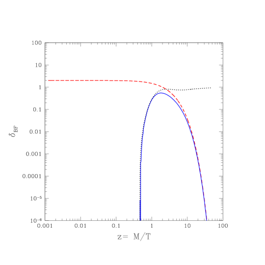
Figure 4: The dashed curve shows the approximation to $\delta_{BF}(z)$ in Eq. (22), while the solid line is the result of a numerical evaluation of the same quantity, which includes the effect of thermal masses and of Fermi–Dirac and Bose–Einstein distributions. The dotted curve shows the result of a numerical calculation of the thermal average $R_{H_{2}}C_{\tilde{L}}$ which multiplies the soft supersymmetry breaking term in Eq. (19).

Concluding the above discussions, we find that the total lepton asymmetry density $Y_{l}=Y_{L}+Y_{\tilde{L}}$ follows the approximate Boltzmann equation:

$${dY_{l}\over dz}=2g_{\Delta}zK\gamma_{D}\left[\tilde{\epsilon}_{l}\delta(z)(Y_{X}-Y_{X}^{eq})+B_{l}(Y_{x}-2{Y_{X}^{eq}\over Y_{l}^{eq}}Y_{l})\right]$$ (23)

where $g_{\Delta}=6$ counts the total number of triplet components generating the lepton asymmetry and $\delta(z)\equiv\delta_{BF}(z)+\delta_{soft}$. In the above equation, the number $K=\Gamma_{\pm}/H_{1}$ takes the minimal value of $K=32$ for $|h|=|\lambda_{2}|\gg|\lambda_{1}|$ as we have the relation softT ;

$$K=32\,{|h|^{2}+|\lambda_{2}|^{2}\over 2|h||\lambda_{2}|}\left({|m_{\nu}|\over 0.05\mbox{ eV}}\right)\,.$$ (24)

As one goes away from the minimum value of $K$ with $|h|\neq|\lambda_{2}|$, the quantity $\tilde{\epsilon}_{l}$ in Eq. (21) gets suppressed. Furthermore, one realizes that the resulting lepton asymmetry is maximized in case of $B_{L,\tilde{L}}=B_{H_{2},\tilde{H}_{2}}\gg B_{H_{1},\tilde{H}_{1}}$ with $|h|=|\lambda_{2}|\gg|\lambda_{1}|$, in which case the Boltzmann equation for the lepton asymmetry takes the simplest form of

$${dY_{l}\over dz}=2g_{\Delta}zK\gamma_{D}\left[\tilde{\epsilon}_{l}\delta(z)(Y_{X}-Y_{X}^{eq})-{Y_{X}^{eq}\over Y_{l}^{eq}}Y_{l}\right]$$ (25)

Let us now note that, taking the resonance condition $B=\Gamma_{\pm}$, one finds the maximal value of $\tilde{\epsilon}_{l}={\mbox{Im}(A)\over M}$, which becomes order one for $A\sim M\sim$ TeV.

Figure 5: Final lepton asymmetry produced by triplet decay as a function of $M$. Different curves refer to $\mbox{Im}(A)=1,2,3,4,5$ TeV from bottom to top.

It is now easy to find the approximate solution for $Y_{l}$ from Eq. (25) with the insertion of $Y_{X}$ given in Eq. (11). Both are found to be a fairly good approximation to the numerical solution of the full Boltzmann equations, as expected from our previous discussions. The results of our numerical calculation are shown in FIG. 5 where we plot the final lepton asymmetry as a function of the triplet mass $M$ for $\mbox{Im}(A)$ from 1 to 5 TeV. When $|A|\sim M$, one needs to recover the contributions of order $|A|/M$ which were neglected, e.g., in Eqs. (Soft Leptogenesis in Higgs Triplet Model) and (21). Taking the parameter region, $m_{0}<|A|=\mbox{Im}(A)$, we keep those contributions in the numerical calculations for the curves in FIG. 5. A remark is in order here. For $M\lower 3.01385pt\hbox{$\;\stackrel{{\scriptstyle\textstyle>}}{{\sim}}\;$}10^{10}$ GeV, the annihilation effect becomes irrelevant and the final asymmetry is determined by the decay and inverse decay effects, i.e., by the value of $K$ only, which confirms the result of Ref. hambye05 . One can see this feature in FIG. 5, where the lepton asymmetry as a function of $M$ changes slope at about $M\sim 10^{10}$ GeV. Below this value the annihilation effect sets in, and the final asymmetry is strongly suppressed compared to the value one would obtain by extrapolating the curve with the slope for $M\lower 3.01385pt\hbox{$\;\stackrel{{\scriptstyle\textstyle>}}{{\sim}}\;$}10^{10}$ GeV.

When the trilinear coupling is larger than the triplet mass, $|A|/M\geq$ 1, besides an enhancement of the CP–violating term of Eq.(21), one could expect that the additional contribution to the coupling of the triplet particles to scalar final states enhances the total annihilation rate, increasing substantially the value of the parameter $K$ compared to the amount given by Eq. (24), which is obtained in the limit $|A|/M\ll 1$. As a consequence of this, the consequent additional wash–out effect could in principle suppress the ensuing lepton asymmetry. However, this is not the case due to the fact that, as we have already discussed, the annihilation process freezes out later than inverse decays, so the latter play almost no role in the determination of the epoch when lepton asymmetry production can start. Actually, this epoch starts when decays eventually overcome annihilations, so a higher value of $K$ can slightly anticipate it, leading so to a higher asymmetry instead than a suppression, although this effect is quite mild. This is what we observe in the numerical calculation shown in FIG. 5, where we have assumed as before $|h|=|\lambda_{2}|\gg|\lambda_{1}|$ (in order to maximize the amount of $CP$ violation given by Eq. (21)) and maximized the $CP$–violating phase (i.e., we have assumed Re$(A)=0$).

We also remark that sphaleron interactions are kept in thermal equilibrium even after the electroweak phase transition and freeze out around $T_{sp}=M/z_{sp}\simeq 90$ GeV, so that only the lepton asymmetry produced for $z<z_{sp}$ can be efficiently converted into a baryon asymmetry apos . As shown in FIG. 3, due to the gauge annihilation effect, the lepton asymmetry production is delayed until $z=z_{0}\simeq 20$. For low values of $M$ ($\sim$ a few TeV) one can have $z_{sp}<z_{0}$, which implies a suppression in the final lepton asymmetry. This explains the fast rise at low values of $M$ of all the curves in FIG.5. On the other hand, the dips observed in the final asymmetry for $M\sim 20|A|$ correspond to the case when the two contributions $\delta_{BF}$ and $\delta_{soft}$ in Eq. (21) are of the same order and cancel. This dip separates the two regions where $\delta_{BF}$ or $\delta_{soft}$ dominates in the determination of the final asymmetry. As shown in FIG. 5, the CP–violating contribution from the soft supersymmetry breaking term $\delta_{soft}$ in Eq. (19) can strongly enhance the final lepton asymmetry at low values of $M$. As a result, it is evident that the required baryon asymmetry can be reached whenever $A$ and $M$ are in the multi-TeV region.

Before concluding our work, let us remark some experimental consequences of the model at future colliders. As shown above, successful baryogenesis requires a TeV-scale triplet mass and Yukawa couplings of the same order, $h\sim\lambda_{2}\sim\sqrt{m_{\nu}M/v_{2}^{2}}\sim 10^{-6}$. Thus, all the low-energy lepton flavor violating processes like $\mu\to e\gamma$ or $\mu\to 3e$ are highly suppressed chun03 . On the other hand, future accelerators have a potential to produce such Higgs triplets, in particular, the peculiar doubly charged component through the Drell-Yan processes gunion . Then, various features of the model can be checked by observing the branching ratios of the triplet decay to lepton and Higgsino pairs, in particular, $\Delta^{--}\to l^{-}_{i}l^{-}_{j},\tilde{H}_{2}^{-}\tilde{H}_{2}^{-}$, allowing also to study neutrino mass patterns chun03 .

In conclusion, we have investigated baryogenesis assuming the minimal supersymmetric Higgs triplet model as the origin of neutrino masses and mixings. This model, with only one pair of triplets, can provide a mechanism for soft leptogenesis employing a CP violating phase and a resonant behavior in the supersymmetry breaking sector. Our analysis shows that the original soft leptogenesis, relying on the supersymmetry breaking effect proportional to the small difference between boson and fermion statistics at finite temperature cannot produce the right amount of baryon asymmetry due to the gauge annihilation effect. In particular, we have calculated the full gauge–annihilation cross section including all the relevant supersymmetric intermediate and final states, as well as coannihilations with the fermionic superpartners of the triplets, finding that this effect strongly suppresses the resulting lepton asymmetry. On the other hand, the contribution of soft supersymmetry breaking terms, particularly a sizable value for the $Im(A)$ parameter, can enhance the lepton asymmetry to provide successful leptogenesis if the triplet mass is in the TeV range. In this case, the model predictions can be tested in future colliders by searching for a very clean signal, e.g., from the production and decay of doubly charged Higgs bosons.

Appendix A Appendix

In this appendix we give the detailed expression for the the annihilation cross section shown in compact form in Eq.(10), and calculated from the diagrams (a)–(s) of FIG. 1. In the following, masses of light particles are neglected, while we assume a common mass $M$ for the triplets and their supersymmetric partners. The reduced cross section introduced in Eq. (10) is defined as:

$$\sigma(t)\equiv\frac{1}{2g_{2}^{4}}\frac{1}{3}\sum\int d\!\cos\theta\,|{\cal M}|^{2},$$

in terms of the integrated squared amplitude, averaged over the initial triplet state (hence the factor 1/3) and summed over the coannihilating particles, given by:

$$\frac{1}{3}\sum\int d\!\cos\theta\,|{\cal M}|^{2} = \frac{4}{3}\sum_{a}tr(T_{a})^{2}tr\left(\frac{\tau_{a}}{2}\right)^{2}\left[F_{(a)+(h)}+F_{(b)+(g)}+F_{(i)}+F_{(l)}\right]+$$ (26)

$$+ \frac{4}{3}\sum_{ab}\left\{tr(T_{a}^{2}T_{b}^{2})\left[F_{(c)+(d)+(e)}+F_{(n)+(o)}+F_{(p)+(q)+(r)}\right]+\right.$$

$$+ \left.8f_{abc}f_{abc}\left[F_{(f)}+F_{(m)}+F_{(s)}+F^{\prime}_{(d)}\right]\right\}\,,\quad\mbox{where}$$

$$F_{(a)+(h)}=\frac{\beta^{2}}{3},\;\;F_{(b)+(g)}=\frac{\beta^{2}}{6},\;\;F_{(i)}=\frac{1}{2},\;\;F_{(l)}=1,\;\;F^{\prime}_{(d)}=-\frac{1}{2},\;\;F_{(s)}=-1$$

$$F_{(c)+(d)+(e)}=2+2\left[1-\beta^{2}+\frac{\beta^{4}-1}{2\beta}\ln\frac{1+\beta}{1-\beta}\right],\;\;\;\;F_{(n)+(o)}=2+2\left[-2+\frac{1}{\beta}\ln\frac{1+\beta}{1-\beta}\right],$$

$$F_{(p)+(q)+(r)}=4+2\left[-2+\frac{1}{\beta}\ln\frac{1+\beta}{1-\beta}\right]\;\;\;\;F_{(f)}=\left[1-\frac{5}{6}\beta^{2}-\frac{(\beta^{2}-1)^{2}}{2\beta}\ln\frac{1+\beta}{1-\beta}\right],$$

$$F_{(m)}=\frac{\beta^{2}}{3}+\left[1+\frac{\beta^{2}-1}{2\beta}\ln\frac{1+\beta}{1-\beta},\right].$$

In the last equation we have kept within squared parentheses quantities that vanish for $\beta\rightarrow 0$, and the subscripts refer to the contributing Feynman diagrams listed in Fig. 1. In Eq. (26), $T_{a}$ and $\tau_{a}/2$ are the SU(2)$\times$ U(1) group generators for the triplet and doublet representations and $f_{abc}$ are the structure constants. Assuming the minimal supersymmetric Standard Model particle content, the traces are given by:

$$\frac{1}{3}\sum_{a}tr(T_{a})^{2}tr({\tau_{a}\over 2})^{2}=g_{2}^{4}(14+11t_{w}^{4}),\;\;\;\frac{1}{3}\sum_{ab}tr(T_{a}^{2}T_{b}^{2})=g_{2}^{4}(4+4t_{w}^{2}+t_{w}^{4}),$$ (27)

and $\sum_{ab}f_{abc}f_{abc}=6g_{2}^{4}$.

Since annihilation decouples for $z\gg 1$, the integral in Eq. (9) can be approximated by making use of the following low-temperature expansion:

$$\int^{\infty}_{1}\!\!dt\,\frac{K_{1}(2zt)}{[zK_{2}(z)]^{2}}\,t^{2}\beta(t)\,\sigma(t)\simeq\frac{1}{2z^{3}}\left[b_{0}+\frac{b_{1}}{z}+...\right],$$ (28)

where $$b_{0}=47+32t_{w}^{2}+\frac{49}{2}t_{w}^{4}\quad\mbox{and}\quad b_{1}=-\frac{3}{2}\left(\frac{98}{3}+32t_{w}^{2}+19t_{w}^{4}\right).$$ (29)

Although for our results we used a numerical integration of Eq.(9), we have checked that the above approximation leads to a good fit to the full numerical calculation for $z\lower 3.01385pt\hbox{$\;\stackrel{{\scriptstyle\textstyle>}}{{\sim}}\;$}$ 10, an interval that safely includes the range of $z$ relevant for the present analysis. We finally notice that the annihilation amplitude increases sizably in the supersymmetric theory compared to the Standard Model case, in significant excess of the factor O(2) suggested by a naïf expectation. In fact, the value of $b_{0}$ in Eq. (29) is almost 8 times larger than the Standard Model value $b_{0}=6+8t_{W}^{2}+2t_{W}^{4}$ coming from the diagrams (c)–(f). Such an enhancement is mainly due to a larger number of available final states for the diagrams (i) and (l), corresponding to the “contact term” for scalars and to triplet–striplet annihilation to gauginos, respectively.

References

(1)
(2)
M. Fukugita and T. Yanagida, Phys. Lett. B174, 45 (1986).
(3) R. Barbieri, D.V. Nanopolous, G. Morchio and
F. Strocchi, Phys. Lett. B 90, 91 (1980); M. Magg and Ch. Wetterich, Phys. Lett. B 94, 61 (1980); J. Schechter and
J. W. F. Valle, Phys. Rev. D22 (1980) 2227; T. P. Cheng and
L. F. Li, Phys. Rev. D 22, 2860 (1980); R.N. Mohapatra and G.
Senjanovic, Phys. Rev. D 23, 165 (1981); G. Lazarides,
Q. Shafi and C. Wetterich, Nucl. Phys. B 181, 287 (1981).
(4)
E. Ma and U. Sarkar, Phys. Rev. Lett. 80, 5716 (1998); T. Hambye, E. Ma,
U. Sarkar, Nucl. Phys. B602, 23 (2001); A. S. Joshipura, E. A. Paschos, W.
Rodejohann, Nucl. Phys. B611, 227 (2001); JHEP 0108, 029 (2001).
(5)
P. O’Donnell and U. Sarkar, Phys. Rev. D49, 2118 (1994); G. Lazarides
and Q. Shafi, Phys. Rev. D58, 071702 (1998) ; E.J. Chun and S.K. Kang,
Phys. Rev. D63, 097902 (2001); T. Hambye and G. Senjanovic,
Phys. Lett. B582, 73 (2004); W. Rodejohann, hep-ph/0403236; P. Gu and X.
Bi, hep-ph/0405092; S. Antusch and S. King, hep-ph/0405093;
hep-ph/0507333; W. Guo, hep-ph/0406268.
(6)
Y. Grossman, T. Kashti, Y. Nir and E. Roulet,
Phys. Rev. Lett. 91, 251801 (2003); JHEP 0411, 080 (2004); G. D’Ambrosio,
G.F. Giudice and M. Raidal, Phys. Lett. B575, 75 (2003).
(7)
E. J. Chun, Phys. Rev. D69, 117303 (2004); Y. Grossman, R. Kitano and H.
Murayama, hep-ph/0504160.
(8)
G. D’Ambrosio, T. Hambye, A. Hektor, M. Raidal and A. Rossi,
Phys. Lett. B 604, 199 (2004).
(9)
J. N. Fry, K. A. Olive and M. S. Turner,
Phys. Rev. D 22, 2977 (1980).
(10)
T. Hambye, M. Raidal and A. Strumia, hep-ph/0510008.
(11)
J.F. Gunion, J. Grifols, A. Mendez, B. Kayser and F. Olness,
Phys. Rev. D40, 1989 (1546);
R. Vega and D. Dicus, Nucl. Phys. B329, 533 (1990);
J.F. Gunion, R. Vega and J. Wudka, Phys. Rev. D42, 1673 (1990);
R. Godbole, B. Mukhopadhyaya and M. Nowakowski, Phys. Lett. B352, 388 (1995);
K. Cheung, R. Phillips and A. Pilaftsis, Phys. Rev. D51, 4731 (1995);
K. Huitu, J. Maalampi, A. Pietila and M. Raidal,
Nucl. Phys. B487, 27 (1997);
T.G. Rizzo, Phys. Rev. D45, 42 (1992);
N. Lepore, B. Thorndyke, H. Nadeau and D. London,
Phys. Rev. D50, 2031 (1994);
J.F. Gunion, C. Loomis and K.T. Pitts, hep-ph/9610237;
B. Dion et. al., Phys. Rev. D59, 075006 (1999);
A. Datta and A. Raychaudhuri, Phys. Rev. D62, 055002 (2000);
E. Ma, M. Raidal and U. Sarkar, Phys. Rev. Lett. 85, 3769 (2000); Nucl. Phys. B615, 313 (2001).
(12)
E. J. Chun, K.Y. Lee and S.C. Park, Phys. Lett. B 566, 142
(2003); A. Akeroyd and A. Aoki, Phys. Rev. D72, 035011 (2005).
(13)
L. Boubekeur, T. Hambye and G. Senjanovic, Phys. Rev. Lett. 93, 111601 (2004).
N. Sahu and U.A. Yajnik, Phys. Rev. D71, 023507 (2005); hep-ph/0509285;
S.F. King and T. Yanagida, hep-ph/0411030;
S. Bray, J.S. Lee, A. Pilaftsis, hep-ph/0508077.
(14)
A. Pilaftsis and T.E.J. Underwood, hep-ph/0506107; E.J. Chun,
hep-ph/0508050.
(15)
A. Rossi, Phys. Rev. D 66, 075003 (2002).
(16)
A. Pilaftsis, Phys. Rev. D56, 5431 (1997).
(17)
L. Covi, E. Roulet, F. Vissani, Phys. Rev. D57, 93 (1998).