A sign change of the moment at $n=0$ of the polarized structure function $g_{1}^{p}$

Abstract

The sum rule for the structure function $g_{1}^{p}$ which is related to the cross section of the photo-production is used to show that a sign change of the integral corresponding to the appropriately defined moment at $n=0$ where the integral is cut at the point $x=x_{c}(Q^{2})$ occurs at very small $Q^{2}$ near $Q^{2}\sim 0.09$(GeV/c)² and $x_{c}\sim 0.024$. This fact shows that the origin of the sign difference between the Ellis-Jaffe sum rule and the Drell-Hearn-Gerasimov sum rule lies in the rapid change of the elastic contribution at low $Q^{2}$ which is compensated by the inelastic contribution to satisfy the sum rule at $n=0$. Hence it occurs at very small $Q^{2}$.

The fact that the sign of the Drell-Hearn-Gerasimov sum ruleDrell ; Ger and that of the Ellis-Jaffe sum ruleEllis was different had motivated the study of these sum rules and the spin structure functions $g_{1}$ and $g_{2}$ at low $Q^{2}$ from both the experiment and the theoryXi ; Bur ; Dres . The Drell-Hearn-Gerasimov (DHG) sum rule stands on the sound theoretical footings. It is based on the general principles such as causality and unitarity. However, since this sum rule holds only at $Q^{2}=0$, a theoretical framework which can treat the region $Q^{2}\neq 0$ in a non-perturbative way with a similar generality as the DHG sum rule is necessary to study the origin of the sign change. Many years ago, the sum rules for the structure functions $g_{1}^{p}$ and $g_{1}^{n}$ which were related to the cross sections of the photo-production were derivedkore . These sum rules were based on the general principles as in the case of the DHG sum rule but corresponded to the moment at $n=0$ of the polarized structure functions $g_{1}$ and $g_{2}$. Hence, compared with the DHG sum rule, they depended more on the high energy behavior of the structure functions and the cross sections of the photo-production. In this paper, using the phenomenological study of the high energy behavior of these quantitySim , we transform the sum rules which are heavily related to the behavior in the very high energy region into the ones at low energy which can be accessible by the experiment, and show that at very small $Q^{2}$ there is a sign change of the appropriately defined moment at $n=0$ of the structure function $g_{1}^{p}$.

Let us first briefly explain how the sum rules can be obtained. The Deser-Gilbert-Sudarshan(DGS) representation which incorporates both causality and the spectrum conditions for the hadron has been of great value in the investigation of the one-particle connected matrix element of the current commutatorDGS ; Con . If the lowest mass $M_{s}$ in the $s$ channel and that of the $M_{u}$ in the $u$ channel satisfys the condition $m\leq(M_{s}+M_{u})/2$ where $m$ is the mass of the hadron of the one-particle state, this representation can be generalized to the product of the currents hence to the anticommutation relation of them. The stable hadron such as the nucleon satisfys the spectral condition. Then, we can consider the restriction of the current commutator and the current anticommutator to the null-plane with the same weight functions in the DGS representation, and using information of the current commutation relation based on the canonical quantization on the null-plane, we see that which terms in the DGS representation remain at the null-planekore80 ; kore84 ; kore93 . In this way, we find that the anticommutaion relation on the null-plane becomes

$$<p|\{J_{a}^{+}(x),J_{b}^{i}(0)\}|p>_{c}\delta(x^{+})$$ (1)

$$= <p|\{s^{+\beta i\alpha}\partial_{\alpha}[\Delta^{(1)}(x)G_{c\beta}(x|0)]-2g^{+\alpha}g^{i\beta}[\partial_{\alpha}[\Delta^{(1)}(x)]G_{c\beta}(x|0)$$

$$- \epsilon^{+i\alpha\beta}\partial_{\alpha}[\Delta^{(1)}(x)G_{c\beta}^{5}(x|0)]\}|p>_{c},$$

where $\Delta^{(1)}(x)$ and $\partial^{+}\Delta^{(1)}(x)$ read $(-1/2\pi)\ln|x^{-}|\delta(\vec{x}^{\bot})\delta(x^{+})$ and
$(-1/2\pi)P(1/x^{-})\delta(\vec{x}^{\bot})\delta(x^{+})$ respectively, and $G_{c}^{\beta}(x|0)$ and $G_{c}^{5\beta}(x|0)$ are decomposed as the symmetric and the antisymmetric combinations as

$$G_{c}^{\beta}(x|0)=d_{abc}A_{c}^{\beta}(x|0)+f_{abc}S_{c}^{\beta}(x|0),$$ (2)

$$G_{c}^{5\beta}(x|0)=d_{abc}S_{c}^{5\beta}(x|0)-f_{abc}A_{c}^{5\beta}(x|0).$$ (3)

Then the connected matrix elements are defined as

$$<p|S_{a}^{\mu}(x|0)|p>_{c}=p^{\mu}S_{a}(p\cdot x,x^{2})+x^{\mu}\bar{S}_{a}(p\cdot x,x^{2}),$$ (4)

$$<p|S_{a}^{5\mu}(x|0)|p>_{c}=s^{\mu}S_{c}^{5}(p\cdot x,x^{2})+p^{\mu}\bar{S}_{a}(p\cdot x,x^{2})+x^{\mu}(x\cdot s)\tilde{S}_{a}(p\cdot x,x^{2}),$$ (5)

where $2s^{\mu}=\bar{u}(p)\gamma^{\mu}\gamma^{5}u(p)$ with $s\cdot p=0,s^{2}=-1$ and we set $m_{N}=1$ for simplicity and similar definitions for the antisymmetric bilocal quantities. Intuitively, the bilocal quantity in Eqs.(2) and (3) can be interpreted as the bilocal currents constructed by the quark bilinear. However, it should be noted that these quantities are defined only as the connected one-particle matrix elements as given on the right side of Eqs.(4) and (5), hence we need no explicit form of the bilocal quantities for the derivation of the sum rule.

The antisymmetric part of the hadronic tensor for the electromagnetic current is defined as

$$\widetilde{W}_{\mu\nu}^{ab} = \frac{1}{4\pi}\int d^{4}x\exp(iqx)<p,s|\{J_{\mu}^{a}(x),J_{\nu}^{b}(0)\}|p,s>_{c}$$ (6)

$$= i\epsilon_{\mu\nu\lambda\sigma}q^{\lambda}s^{\sigma}\tilde{G}_{1}^{ab}+i\epsilon_{\mu\nu\lambda\sigma}q^{\lambda}(\nu s^{\sigma}-q\cdot sp^{\sigma})\tilde{G}_{2}^{ab}.$$

The structure function $\tilde{G}_{i}$ for $i=1,2$ has opposite crossing property under $q\to-q,a\leftrightarrow b$ and $\mu\leftrightarrow\nu$ compared with the usual one defined by the current commutation relation. Now following the standard method to get the fixed-mass sum rule in the null-plane formalismDJT , we obtain the two sum rules

$$\int_{0}^{1}\frac{dx}{x}g_{1}^{ab}(x,Q^{2}) = \frac{-1}{8\pi}d_{abc}\int_{-\infty}^{\infty}d\alpha\ln|\alpha|[S_{c}^{5}(\alpha,0)+\alpha\bar{S}_{c}^{5}(\alpha,0)],$$ (7)

$$\int_{0}^{1}\frac{dx}{x}g_{2}^{ab}(x,Q^{2}) = \frac{1}{8\pi}d_{abc}\int_{-\infty}^{\infty}d\alpha\alpha\ln|\alpha|\bar{S}_{c}^{5}(\alpha,0),$$ (8)

where we set $\nu=p\cdot q,\alpha=p\cdot x,-q^{2}=\vec{q}_{\bot}^{2}=Q^{2}$, and use the fact that ,in the $s$ channel ,$\tilde{G}_{i}$ is the same as the structure function $G_{i}$ defined by the current commutation relation and that $g_{1}^{ab}=\nu G_{1}^{ab}$ and $g_{2}^{ab}=\nu^{2}G_{2}^{ab}$. Since the right side of Eqs.(7) and (8) is $Q^{2}$ independent, we obtain

$$\int_{0}^{1}\frac{dx}{x}g_{1}(x,Q^{2})=\int_{0}^{1}\frac{dx}{x}g_{1}(x,Q_{0}^{2})$$ (9)

for any $Q^{2}$ and $Q_{0}^{2}$. Similar relation exists for the structure function $g_{2}$ and $g_{1}+g_{2}$.

The sum rule (9) depends strongly on the small $x$ behavior of the structure function $g_{1}$. The Regge theory predicts as $g_{1}\sim\beta x^{-\alpha_{i}(0)}$ with $\alpha_{i}(0)\leq 0$ where $i$ denotes $a_{1}$ and $f_{1}$ trajectory. In this case, the sum rule is convergent except at $\alpha_{i}=0$. The extrapolation of the DGLAP fit to the unmeasured small $x$ region have large ambiguitygrsv . The double logarithmic $(log(1/x))^{2}$ resummation give more singular behavior than the Regge theorybade . The latter cases shows the sum rule (9) is divergent. Though, whether the sum rule diverges or not can not be judged rigorously by these discussions, in view of these situations, it is important to discuss the regularization of the sum rule and give it a physical meaning even when the sum rule is divergent. Now,the formally divergent sum rule of the forward direction in the null-plane formalism was known to be regularized by the analytical continuation of the sum rule in the non-forward directiondealwis ; DP . This method was further developed to the current anticommutation relation on the null-plane in Ref.kore84 ; kore93 ; kore98 . We consider the non-forward matrix element corresponding to the reaction ’current($q_{1}$)+nucleon($p_{1}$) $\to$ current($q_{2}$)+nucleon($p_{2}$)’, where we define $K=(q_{1}+q_{2})/2,P=(p_{1}+p_{2})/2,\Delta=q_{2}-q_{1},\Delta^{2}=t,q_{1}^{2}=q_{2}^{2},p_{1}^{2}=p_{2}^{2},$ and $S^{\mu}=\bar{(p_{2}s_{2})}\gamma^{\mu}\gamma^{5}u(p_{1}s_{1})/2$. The explicit expression of the matrix element of the current anticommutation relation on the null-plane was given for the case $\mu=+,\nu=+$. The same reasoning can be done for the case $\mu=+,\nu=i$. Since we need kinematics of the spin-dependent part in doing this, we explain it. The spin-dependent part for the conserved vector current has been known to be expressed by the 13 structure functions.DP In case of the $q_{1}^{2}=q_{2}^{2}$ and $p_{1}^{2}=p_{2}^{2}$ in this paper, 5 structure functions becomes zero under the time-reversal invariance. Among the remaining 8 structure functions, the tensor structure of 6 structure functions are proportional to $\Delta$. Hence only 2 structure functions are left. We can take these two structure functions as the ones which exactly become $\tilde{G}_{1}$ and the $\tilde{G}_{2}$ in the forward matrix element and separate out the terms which remain in the forward limit. Now, under this kinematical structure, since $P,K,\Delta$ are independent variables we obtain the sum rules of the same forms as Eqs.(7)-(9) in the non-forward case. Each quantity which appears in the sum rules (7)-(9) is replaced by the quantity in the non-forward one(see Eq.(2.11) and Eq.(4.1) in Ref.kore84 ). Then by assuming a moving pole or cut, we analytically continue them to the forward direction. Since the sum rules take the same form as the forward ones, we can effectively do this manipulation by using the sum rules in the forward direction by introducing the parameter which reflects the moving pole or cut. In case of the sum rule (9), we rewrite it as

$$\int_{0}^{1}\frac{dx}{x}\{g_{1}(x,Q^{2})-f(x,Q^{2})\}+\int_{0}^{1}\frac{dx}{x}f(x,Q^{2})$$ (10)

$$= \int_{0}^{1}\frac{dx}{x}\{g_{1}(x,Q_{0}^{2})-f(x,Q_{0}^{2})\}+\int_{0}^{1}\frac{dx}{x}f(x,Q_{0}^{2}),$$

where $f(x,Q^{2})$ is the term which includes a possible divergent piece in $g_{1}(x,Q^{2})$. Let us consider the simple pole case as $\alpha(0,\epsilon)=a-\epsilon$, and set $f(x,Q^{2})=\beta(Q^{2})x^{-\alpha(0,\epsilon)}+f_{1}(x,Q^{2})$. The $\epsilon$ is a parameter which reflects the moving pole and proportional to $t$ in the non-forward case. The cases where more moving poles which give divergent behavior in the forward exist can be done simply by repeating the argument below with a minor trivial modification. We first take $\epsilon>a$ and obtain

$$\int_{0}^{1}\frac{dx}{x}f(x,Q^{2})=\frac{\beta(Q^{2})}{\epsilon-a}+\int_{0}^{1}\frac{dx}{x}f_{1}(x,Q^{2}),$$ (11)

where the integral over $f_{1}$ on the right hand side of Eq.(11) is finite in the limit $\epsilon\to a$ and $\epsilon\to 0$. Then we take out the pole from both sides of Eq.(10) by obtaining the condition $\beta(Q^{2})=\beta(Q^{2}_{0})$, and take the limit $\epsilon\to 0$. Thus we obtain

$$\int_{0}^{1}\frac{dx}{x}\{g_{1}(x,Q^{2})-f(x,Q^{2})\}$$ (12)

$$= \int_{0}^{1}\frac{dx}{x}\{g_{1}(x,Q_{0}^{2})-f(x,Q_{0}^{2})\}+\int_{0}^{1}\frac{dx}{x}\{f(x,Q_{0}^{2})-f(x,Q^{2})\},$$

where we have replaced the integral over $f_{1}$ to $f$ in the final result under the recognition that the coefficient of a possible divergent piece in $g_{1}$ is $Q^{2}$ independent. Practically, we do not care about this condition since it is necessary only in the $x\to 0$ limit. In this sense, as far as we can find a large cancellation in the high energy region, Eq.(12) can be considered to be valid.

Now, let us first consider the results of the sum rule (9) for the proton target when it is convergent. In the sum rule, $g_{1}$ in general includes the elastic contribution. Since our concern here lies in the behavior of $g_{1}$ in the low $Q^{2}$ region and we take $Q_{0}^{2}=0$ on the right side of Eq.(9), we keep the Born contribution on both sides of Eq.(9)com , and obtain

$$\int_{0}^{1}\frac{dx}{x}g_{1}^{p}(x,Q^{2})=B(Q^{2})-\frac{1}{8\pi^{2}\alpha_{em}}\int_{\nu_{0}}^{\infty}d\nu\{\sigma_{3/2}^{\gamma p}-\sigma_{1/2}^{\gamma p}\},$$ (13)

with

$$B(Q^{2})=\frac{1}{2}\{F_{1}^{p}(0)(F_{1}^{p}(0)+F_{2}^{p}(0))-F_{1}^{p}(Q^{2})(F_{1}^{p}(Q^{2})+F_{2}^{p}(Q^{2}))\},$$ (14)

where we use the relation at $Q^{2}=0$

$$G_{1}^{p}(\nu)=\frac{-1}{8\pi^{2}\alpha_{em}}\{\sigma_{3/2}^{\gamma p}-\sigma_{1/2}^{\gamma p}\}.$$ (15)

Here the Dirac form factor takes the values $F_{1}^{p}(0)=1$ and $F_{2}^{p}(0)=1.79$, and we give the nucleon mass dependence explicitly.

Now $B(Q^{2})$ is well known experimentally. We plot it in Fig.1 by using the standard dipole fitArn

$$G_{E}^{p}=\frac{1}{(1+\frac{Q^{2}}{0.71})^{2}},G_{M}^{p}=\mu_{p}G_{E}^{p},$$ (16)

where the anomalous magnetic moment $\mu_{p}=2.793$. The relation between the Dirac form factor and the Sacks ones are $G_{M}^{p}=F_{1}^{p}+F_{2}^{p}$ and $\displaystyle{G_{E}^{p}=F_{1}^{p}-\frac{Q^{2}}{4m_{N}^{2}}F_{2}^{p}}$.

Figure 1: The difference of the Born terms as given by the $B(Q^{2})$

Let us turn to the estimate of the integral of the cross section of the photo-production and rewrite the sum rule (13) by applying Eq.(12). Recently,the measurement of the $\Delta\sigma=\sigma_{3/2}-\sigma_{1/2}$ was reportedahrens ; dutz . According to these, we can estimate the integral on the right side of Eq.(13) up to $E\sim 2$ GeV directly with use of the experimental value where $E$ is the energy of the photon in the laboratory frame. The contribution above this comes both from the resonances and the non-resonant terms. Though the contribution from the former is small, the one from the latter is expected to be very large. On the other hand, to estimate the left side of Eq.(13), we need information of the $g_{1}$ in the very small $x$ region which is also expected to give a large contribution. In the small $Q^{2}$ region, if we take a sufficiently large energy, high energy behavior of the total cross section of the photo-production may coincide with that of the $g_{1}$ with exactly the same proportional constant as given in Eq.(15). In fact, there is a phenomenological parameterization which has this propertySim . Then, the possible large contributions from both sides of Eq.(13) may cancel out. This is a situation where the regularized sum rule (12) can be used. Thus, by setting $\nu=m_{N}E$ in the laboratory frame, for arbitrary $Q^{2}$, we equate $f(x,Q^{2})$ in the sum rule (12) as $g_{1}(x,Q^{2})$ below $x=x_{c}$ and 0 above it where $x_{c}=Q^{2}/2\nu_{c}^{Q}$,$\nu_{c}=m_{N}E_{c}$, and $\nu_{c}^{Q}=\nu_{c}+Q^{2}/2$ with $E_{c}=2$ GeV. Then we divide the integral from $0$ to $x_{c}(Q^{2})$ and $x_{c}(Q^{2})$ to $1$ for the $g_{1}(x,Q^{2})$ and $f(x,Q^{2})$ and from $0$ to $x_{c}(Q_{0}^{2})$ and $x_{c}(Q_{0}^{2})$ to $1$ for the $g_{1}(x,Q_{0}^{2})$ and $f(x,Q_{0}^{2})$. Using the fact that the $g_{1}(x,Q^{2})=f(x,Q^{2})$ below $x=x_{c}(Q^{2})$ and $g_{1}(x,Q_{0}^{2})=f(x,Q_{0}^{2})$ below $x=x_{c}(Q_{0}^{2})$, we can rewrite the sum rule (12). Then, by taking the $Q_{0}^{2}=0$ and using the relation (15), the sum rule(12) where the Born term is separated out is given as

$$\int_{x_{c}}^{1}\frac{dx}{x}g_{1}^{p}(x,Q^{2})=B(Q^{2})-\frac{1}{8\pi^{2}\alpha_{em}}\int_{\nu_{0}}^{\nu_{c}}d\nu\{\sigma_{3/2}^{\gamma p}-\sigma_{1/2}^{\gamma p}\}+K(E_{c},Q^{2}),$$ (17)

where

$$K(E_{c},Q^{2})=\frac{1}{8\pi^{2}\alpha_{em}}\int_{\nu_{c}}^{\infty}d\nu\{\sigma_{1/2}^{\gamma p}-\sigma_{3/2}^{\gamma p}\}-\int_{\nu_{c}^{Q}}^{\infty}\frac{d\nu}{\nu}g_{1}^{p}(x,Q^{2}).$$ (18)

Here the integral over $\nu$ in Eq.(18) should be understood to be done after we subtract the high energy behavior of both the photoproduction and the $g_{1}^{p}(x,Q^{2})$. The sum rule (17) is the regularized version of the sum rule (13), where the high energy contribution is subtracted out. We take the $g_{1}^{p}$ in the $K(E_{c},Q^{2})$ as the non-resonant contribution $g_{1}^{non-res.}$ in Ref.Sim . We neglect the resonant contribution above $E_{c}$, since inclusion of these contribution does not affect the following discussions. We further approximate the $g_{1}^{non-res.}$ as $g_{1}^{non-res.}=g^{\Delta\sigma}$ where $g^{\Delta\sigma}$ is the contribution arising from the transverse asymmetry $A_{1}(x,Q^{2})$ and also defined in Ref.Sim . The approximation here is equivalent to neglect $g_{2}$ in the transverse asymmetry, and its effect is negligible in the evaluation of the $K$ above $E_{c}=2$GeV. Further, for $Q^{2}<0.1$(GeV/c)², we cut the integral in $K$ at $E=100$GeV since the integrand can almost be regarded as zero in this energy region. Under these approximations, for example,we obtain $K(2,0.05)\sim-0.014$ and $K(2,0.1)\sim-0.027$.para Thus there is a large cancellation here. On the other hand, using the experimental data given in Ref.dutz , we obtain

$$\frac{m_{N}}{8\pi^{2}\alpha_{em}}\int_{E_{0}}^{2}dE\{\sigma_{3/2}^{\gamma p}-\sigma_{1/2}^{\gamma p}\}\sim 0.45.$$ (19)

By calculating $K(2,Q^{2})$ for each $Q^{2}$, we plot the left-hand side of Eq.(17) as a function of $Q^{2}$ in Fig.2. The dotted curve (a) is the one where the contribution from $K(2,Q^{2})$ is neglected and the curve (b) is the one where the contribution from $K(2,Q^{2})$ is included. From it we find that the integral

$$\int_{x_{c}}^{1}\frac{dx}{x}g_{1}^{p}(x,Q^{2})$$ (20)

become zero in the region near $Q^{2}\sim 0.09$(GeV/c), where $x_{c}=0.024$.

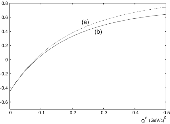
Figure 2: The estimate of the left-hand side of Eq.(17). The dotted curve (a) is the one given by the Born contribution $B(Q^{2})$ and Eq.(19) by neglecting $K(2,Q^{2})$. The curve (b) is the one including the contribution from $K(2,Q^{2})$.

Now we can use the parameters in Ref.Sim not only to show the smallness of the $K(E_{c},Q^{2})$ at small $Q^{2}$ but also to check the right hand side of Eq.(19). Since the value is slightly different from 0.45 as given in Eq.(19), we find that the zero of Eq.(20) occurs at $Q^{2}\sim 0.16$(GeV/c)² with $x_{c}=0.042$. This zero point is a little bit larger than $Q^{2}\sim 0.09$(GeV/c)². However, in this model, we see that this same rapid change of the inelastic contribution of the $g_{1}^{p}$ gives the sign change of the generalized Drell-Hern-Gerasimov sum rule.

In summary, we have shown that the appropriately defined moment at $n=0$ of the polarized structure function $g_{1}^{p}$ defined at the left hand side of Eq.(17) becomes zero at small $Q^{2}$ near $Q^{2}\sim 0.09$(GeV/c)², and that the sign change occurs at this point. Since the Ellis-Jaffe sum rule corresponds to the moment at $n=1$ which is more sensitive to the low energy behavior than the present one at $n=0$, the negative resonance contribution is enhanced in it. Therefore the fact that the moment at $n=0$ change sign shows that the sign of the Drell-Hern-Gerasimov sum rule is opposite to that of the Ellis-Jaffe sum rule. The origin of the sign change is the rapid change of the Born term at low $Q^{2}$ which is compensated by the inelastic contribution. Thus the fact that the rapid change of the Born term is below $Q^{2}<0.5$ (GeV/c)² explains why the sign change occurs at very small $Q^{2}$. The compensation is the reflection of the $Q^{2}$ independence of the moment at $n=0$ as given by the sum rule (9), from which the sum rule (17) is derived. Phenomenological importance of the sum rule (17) lies in the fact that we can investigate the $Q^{2}$ dependence of the resonance structure in the low and the intermediate energy region at low $Q^{2}$ without worrying about the correction from the high energy behavior. Now, the sum rule (17) can be used for any $Q^{2}$. For example, it can be used for the $Q^{2}$ in the deep inelastic region. In this case, the $Q^{2}$ dependent piece in the Born terms rapidly become 0 and hence it can be neglected. On the other hand, we get a large contribution from $K(Q^{2},E_{c})$, if we take $E_{c}=2$ GeV. We need more data in the small $x$ region together with information of the photo-production to see how far the high energy behavior is canceled. If we can find a large cancellation, we take a large $E_{c}$ such that a contribution from $K(Q^{2},E_{c})$ becomes small. In this way, we can extend the analysis of the sum rule (17) to the larger $Q^{2}$ region where the resonance contribution turns to the continuum contribution and study their relation.

References

- (1) S.D.Drell and A.C.Hern, Phys.Rev.Lett. 16,908(1966).
- (2) S.B.Gerasimov, Yadern Fiz.2,598(1965)[Sov.J.Nucl.Phys. 2,430(1966)]
- (3) J.Ellis and R.L.Jaffe, Phys.Rev.D9,1444(1974); ED10,1669(1974).
- (4) V.D.Burkert, Mod.Phys.Lett.A 18, 262(2003).
- (5) B. W. Filippone and Xiangdong Ji, Adv.Nucl.Phys. 26, 1(2001).
- (6) D.Drechel and L.Tiator, nucl-th/0406059.
- (7) S.Koretune, Prog.Theor.Phys.90, 1049 (1993).
- (8) S.Simula, M.Osipenko, G.Ricco and M.Taiuti, Phys.Rev. D65, 034017(2002).
- (9) S.Deser,W.Gilbert,and E.C.G.Sudarshan, Phys.Rev. 115, 731(1959).
- (10) J.M.Cornwell and R.E.Norton, Phys.Rev. 173, 1637(1968); J.M.Cornwall,D.Corrigan, and R.E.Norton, Phys.Rev. D3, 536(1970).
- (11) S.Koretune, Phys.Rev. 21, 820(1980).
- (12) S.Koretune, Prog.Theor.Phys. 72, 821(1984).
- (13) S.Koretune, Phys.Rev. D47, 2690(1993).
- (14) D.A.Dicus,R.Jackiw, and V.L.Teplitze, Phys.Rev. D4, 1733(1971).
- (15) M.Glück, E.Reya, M.Stratmann, and W.Vogelsang, Phys.Rev.D63, 094005(2001).
- (16) B.Badelek, Acta Phys.Polon. B34, 2943 (2003).
- (17) S.P.de Alwis, Nucl.Phys. B43, 579(1972).
- (18) D.A.Dicus and D.R.Palmer, Annals of Phys. 79, 68(1973).
- (19) S.Koretune, Nucl.Phys. B526, 445(1998).
- (20) In the previous paperkore , we take in the deep inelastic region and as 0. Since the Born term becomes negligible in the deep inelastic region, it was kept only on the right side of Eq.(9). Further in the paperkore was two times larger than the usually defined ones given in this paper.
- (21) R.Arnold et al., Phys.Rev.Lett.57, 174(1986).
- (22) Ahrens J, et al.(GDH and A2 Collaborations). Phys.Rev.Lett. 84, 5950(2000);Phys.Rev.Lett. 87, 022003(2001).
- (23) For the explicit equation of ,see Eqs.(22)-(24) and Table I in Ref.[8].
- (24) Dutz H, et al.(GDH Collaboration). Phys.Rev.Lett. 91, 192001(2003).