2.5cm2.5cm2.5cm2.5cm

Pontificia Universidad Católica de Chile

Facultad de Física

CHIRAL DYNAMICS AND PION PROPERTIES AT FINITE TEMPERATURE AND ISOSPIN CHEMICAL POTENTIAL

by

CRISTIÁN LUIS VILLAVICENCIO REYES

A thesis submitted to Facultad de Física, Pontificia Universidad Católica de Chile, in partial fulfillment of the requirements for the degree of Doctor of Philosophy.

Advisor : Dr. Marcelo Loewe Examining Committee : Dr. Jorge Alfaro Dr. Marco A. Díaz Dr. Claudio Dib Dr. Andreas Reisenegger

Agosto, 2004

Santiago – Chile

Abstract

The thermal and density corrections, in terms of the isospin chemical potential $\mu_{\mbox{\tiny I}}$, to the mass of the pions, the decay constant and different condensates are studied in the framework of the $SU(2)$ low energy effective chiral lagrangian at finite temperature in the two phases: The first phase $|\mu_{\mbox{\tiny I}}|<m$ and the second phase $|\mu_{\mbox{\tiny I}}|>m$, being $m$ the tree-level pion mass. As a function of temperature for $\mu_{\mbox{\tiny I}}=0$, the mass remains quite stable, starting to grow for very high values of $T$, confirming previous results. However, there are interesting corrections to the mass when both effects (temperature and chemical potential) are simultaneously present. At zero temperature the $\pi^{\pm}$ should condense when $\mu_{\mbox{\tiny I}}=\pm m_{\pi}$. At finite $T$, the condensed pion acquires a thermal mass in such a way that a mixture, like in a superfluid, of a condensed and normal phase appears.

Preface

There is a reasonable agreement that Quantum Chromodynamics (QCD) is the right theory that explains strong interactions. The QCD degrees of freedom are quark fields and gluon gauge fields, which possess color charge and, up till now, have not been detected as isolated free particles. The theory cannot explain the confinement of the quarks and gluons inside the hadrons, and it is not possible to obtain, in general, analytical solutions, except for processes at high energies or “hard processes” (also equivalent to small distances) where, due to the asymptotic freedom, perturbation theory is possible [GW73b, GW73a, GW74, Pol73]. Non-perturbative methods like the Operator Product Expansion (OPE) and QCD Sum Rules [SVZ79] or the Nambu Jona-Lasinio (NJL) effective model [NJL61] include corrections to the perturbative analysis, with quark-gluons degrees of freedom, in terms of condensates, responsible for the hadronic resonances at low energy. Numerical simulations of QCD on the Lattice [tH78, tH81], on the other side, turn out to be a real non-perturbative approach to the theory, starting from first principles.

Chiral Effective field theories, like the Linear Sigma Model [GML60], the Non-Linear Sigma Model [Wei68] and Chiral Perturbation Theory ($\chi$PT) [Wei79, GL84, GL85], have been a strong and useful tool for understanding QCD at low energies or “soft processes”, since they involve hadronic degrees of freedom preserving the symmetries of QCD and allow us to establish a connection with the concepts of Current Algebra (the precursor of QCD). Among all hadrons, pions play a special role in the dynamics of hadronic matter because they are the lightest hadrons and therefore are produced at a higher rate in high-energy reactions. The discussion of pion dynamics is a precious window to explore the non-perturbative structure of QCD.

In the last 20 years, there has been a special interest in hot and (or) dense processes in scenarios like the early universe, relativistic heavy ion collisions, and inside neutron stars. High energy processes in a thermal bath have been studied in different frames, searching for new phenomena and states of matter like Chiral Symmetry Restoration (see for example [NRZ96]), the Quark-Gluon Plasma [Mul85, KS04, Kod04] and confinement of quarks and gluons into hadrons, Color Glass Condensate [ILM01, FILM02, McL04], etc. In all these cases we deal with different phase transitions. A main problem in this context is to find the appropriate order parameters, in terms of observable quantities associated to the behavior of a quasi-particle in a medium.

The dependence of the pion properties on finite temperature has been studied in a variety of frameworks, such as thermal QCD-Sum Rules [DFL96], Chiral Perturbation Theory at one loop [GL87b] and two loops [Sch93, Tou97], the Linear Sigma Model [Lar86, CL90, DLR94], the Mean Field Approximation [Pis82, BCDC⁺92], the Virial Expansion [LS90, Sch91], etc. There seems to be a reasonable agreement that the pion mass $m_{\pi}(T)$ is essentially independent of $T$, except possibly near the critical temperature $T_{c}$, where $m_{\pi}(T)$ increases with $T$, and that the pion decay constant $f_{\pi}(T)$ vanishes at the critical temperature.

The introduction of in-medium processes via isospin chemical potential has been studied at zero temperature in $\chi$PT [SS01, KT01, STV02a] in both phases ($|\mu_{I}|\lessgtr m_{\pi}$) at tree level.

In-medium properties at finite density have been discussed for a variety of phenomena, as for example, the chiral condensates [PLL⁺03, PLLW03], the anomalous decays of pions and etas [CRK03], etc. As the density increases, both the quark condensates and the decay rates diminish.

Interesting results concerning the structure of the QCD phase diagram, including temperature effects, have been achieved for the case when we have simultaneously baryon chemical potential and isospin chemical potential. Two completely different approaches have confirmed a qualitative change in the phase diagram as soon as the isospin chemical potential starts to grow [TK03, BPRC03]. These problems concerning the structure of the phase transition diagram, have also been handled in the frame of two color QCD in four dimensions (a QCD-like model) [STV02b] as well as in three dimensions [DN03]. The problem with baryonic chemical potential has been considered in the frame of $\chi$PT [AEGN95] and also using the finite pion number chemical potential [AAA02].

Different properties of QCD (or QCD-inspired models) under these kind of circumstances have also been analyzed in the lattice approach. For QCD with three and two colors, extensive work has been carried out [KTS01, KTS02, KS02b, KS02a, KTS03] in connection with the behavior of different order parameters in several phase transitions in the $\mu/T$ plane as, for example, the transition to a diquark phase, the chiral condensate, etc.

Isospin asymmetry does exist in nature in the case of neutron stars. Since 1971, the idea of a pion condensate in the core of neutron stars has been considered in connection with the cooling process of a neutron star (see for example [YP04]). This idea is a motivation to study the behavior of pions at extreme isospin densities, searching for phase transitions and considering the possibility of having such scenario, isospin asymmetric regions, in RHIC and ALICE experiments. Eventually, these considerations are relevant in early stages of the universe.

The main results of this thesis concerns the discussion of thermal radiative corrections, including finite isospin chemical potential role on both pion phases, enlarging in this way the existing literature on the isospin chemical potential effects in the pion phase transitions [STV02b, KS04]. The results of this thesis with respect to the thermal masses and decay constants in the first phase can be found in [LV03] and the behavior of the thermal masses in the second phase in [LV04]. The non-tivial evolution of pion masses and decay constants may have also important phenomenological consequences for the diagnosis of the pion gas, in the central rapidity region of relativistic heavy ion collisions, when looking for signals as dilepton or photo-production.

This thesis is organized as follows: In chapter 1, I will introduce Chiral Perturbation theory, the renormalization procedure involved, and the finite temperature and density formalism. In chapter 2, the derivation of the effective Lagrangian, the propagators necessary for radiative corrections, and the expansion criteria to solve the problem of the non-diagonal propagators in the second phase will be presented. In chapter 3, the self-energy corrections, decay constants, and condensates in the first phase will be derived. Chapter 4 and 5 will be devoted to the calculation of the self-energy corrections and condensates in the regions $\mu_{\mbox{\tiny I}}\gtrsim m$ and $\mu_{\mbox{\tiny I}}\gg m$. Finally, in chapter 6, I will summarize the results and conclusions, presenting also an outlook.

Chapter 1 Introduction

This chapter is a brief introduction about the theories and tools that will be used to compute radiative corrections within a thermal bath for the case of a pure pion gas; i.e., $\chi$PT and Thermo-Field Dynamics.

1.1 Chiral Perturbation Theory

$\chi$PT is a successful effective field theory that makes use of the chiral symmetry, which is an intrinsic symmetry of massless fermions. Since light quarks ($u$, $d$) possess masses of a few MeV (the $s$ quark can also be handled in this frame), it is reasonable to think of them as massless, allowing a separation of the quark fields in right- and left-handed components. Then, it is possible to construct an effective Lagrangian with hadronic degrees of freedom that preserves chiral symmetry. The idea of the construction of an effective theory in this context was first proposed by Weinberg [Wei79].

The chiral symmetry breaking is usually parametrized by a non-vanishing pion decay constant $f_{\pi}$, using Partial Conservation of Axial Current (PCAC) [GML60, Nam60]. According to the Goldstone theorem [GSW62], a consequence of the spontaneous symmetry breaking will be the appearance of massless bosons. In the case of $\chi$PT, where the $SU(N)_{R}\times SU(N)_{L}$ chiral symmetry grou reduces to a $SU(N)_{V}$, $N^{2}-1$ massless bosons appear, according to the number of generators of the group $SU(N)$ that do not annihilate the vacuum. In the case of $SU(2)$, for the two lightest flavors $u$ and $d$, the massless goldstone bosons are associated with the three pion pseudo-scalar fields. In fact pions are pseudo-goldstone bosons, due to the intrinsic mass of the quarks.

In the same way as it happens in the theory of superconductivity, we expect that quarks should form Cooper pairs of bound quark-antiquark states, due to strong attractive interactions, specially if the quarks are massless. The vacuum state with a quark pair condensate is characterized by the order parameter $\langle\bar{q}q\rangle\neq 0$, which also breaks the chiral symmetry, allowing the quarks to acquire effective masses as they move through the vacuum. Then the pions acquire a mass due to the explicit symmetry breaking induced by the small quark masses and also due to the existence of this quark condensate.

One of the advantages of $\chi$PT, for example in the case of two flavors, is that we can forget about the isosinglet scalar field $\sigma$ because it is heavier than the pseudo-scalar fields ($m_{\sigma}\sim(400-1200)MeV$ in comparison with $m_{\pi^{\pm}}\approx 140MeV$). Then, it is possible to concentrate on pion interactions only, in a scenario like a pion gas, especially when dealing with finite-temperature corrections. In effective models, like the linear $\sigma$-model, it is possible to discuss the properties of the $\sigma$-meson, and its influence in the low-energy dynamics [CL90, DLR94]. Here, I will only concentrate on the pion dynamics, dominant when finite temperature and density effects are taken into account.

A new comprehensive review of $\chi$PT can be found in [Sch02].

1.1.1 Chiral Lagrangian

Let us proceed in the frame of the $SU(2)$ chiral perturbation theory. The most general chiral invariant expression for a QCD-extended Lagrangian under the presence of external hermitian-matrix auxiliary fields, has the form

$${\cal L}_{QCD}(s,p,v,a)={\cal L}_{QCD}^{0}+{\cal L}_{QCD}^{A}+\bar{q}\gamma^{\mu}(v_{\mu}+\gamma_{5}a_{\mu})q-\bar{q}(s-i\gamma_{5}p)q,$$ (1.1)

where ${\cal L}_{QCD}^{0}$ is the usual QCD Lagrangian with zero mass, ${\cal L}_{A}$ is the anomalous part and $s$, $p$, $v$, and $a$ are scalar, pseudo-scalar vector and axial external fields defined as

$$\begin{array}[]{cc}v_{\mu}=v_{\mu}^{a}(x)\tau^{a}/2,&\qquad s=s^{0}(x)+s^{a}(x)\tau^{a},\\ a_{\mu}=a_{\mu}^{a}(x)\tau^{a}/2,&\qquad p=p^{0}(x)+p^{a}(x)\tau^{a}\end{array}$$ (1.2)

where $s_{\mu}^{a}$, $p_{\mu}^{a}$, $v_{\mu}^{a}$, $a_{\mu}^{a}$ are real functions and $\tau^{a}$ are the Pauli matrices. Consider the independent local $SU(2)_{R}\times SU(2)_{L}$ transformations of the left- and right-handed quarks in flavor space (chiral transformations)

$$\begin{array}[]{lr}(1+\gamma_{5})q\rightarrow g_{R}(1+\gamma_{5})q,&\qquad\big{(}1-\gamma_{5}\big{)}q\rightarrow g_{L}(1-\gamma_{5})q,\end{array}$$ (1.3)

which induce gauge transformations of the external fields

$$v^{\prime}_{\mu}+a^{\prime}_{\mu} = g_{R}(v_{\mu}+a_{\mu})g_{R}^{\dagger}+ig_{R}\partial_{\mu}g^{\dagger}_{R},$$ (1.4)

$$v^{\prime}_{\mu}-a^{\prime}_{\mu} = g_{L}(v_{\mu}-a_{\mu})g_{L}^{\dagger}+ig_{L}\partial_{\mu}g^{\dagger}_{L},$$ (1.5)

$$s^{\prime}+ip^{\prime} = g_{R}(s+ip)g_{L}^{\dagger}.$$ (1.6)

Then, it is possible to construct a generalized chiral-invariant Lagrangian containing only pion degrees of freedom, where the external fields transform in the same way as in Eq.(1.6). The effective low-energy Lagrangian will be expressed as an expansion in powers of momentum $P$ on a certain scale $\Lambda_{\chi}$,

$${\cal L}_{\chi}={\cal L}_{2}+{\cal L}_{4}+{\cal L}_{6}+\dots+{\cal L}_{\chi}^{A},$$ (1.7)

where ${\cal L}_{n}\sim{\cal O}(P^{n})$ and ${\cal L}_{\chi}^{A}$ is the Wess-Zumino-Witten Lagrangian (the anomaly contribution).

According to Weinberg power counting [Wei79], $\partial,a,v,s,p\sim{\cal O}(P)$. This means that the external momentum must be smaller than a certain scale $\Lambda_{\chi}$ in order to proceed with an expansion in a series of powers of momentum.

We will start with the ${\cal O}(P^{2})$ chiral Lagrangian

$${\cal L}_{2} = \frac{f^{2}}{4}Tr\left[(D_{\mu}U)^{\dagger}D^{\mu}U+U^{\dagger}\chi+\chi^{\dagger}U\right]$$ (1.8)

with

$$D_{\mu}U = \partial_{\mu}U-i[v_{\mu},U]-i\{a_{\mu},U\},$$ (1.9)

$$\chi = 2B(s+ip),$$ (1.10)

$$U = \bar{U}^{\mbox{\tiny$1/2$}}(e^{i\pi^{a}\tau^{a}/f})\bar{U}^{\mbox{\tiny$1/2$}}.$$ (1.11)

At this point, $f$ and $B$ are arbitrary constants with dimension of mass, and $\bar{U}$ is the vacuum expectation value of the unitary-matrix field $U$.

The most general ${\cal O}(P^{4})$ chiral Lagrangian has the form

$${\cal L}_{4} = {\textstyle\frac{1}{4}}l_{1}\left(Tr\left[(D_{\mu}U)^{\dagger}D^{\mu}U\right]\right)^{2}$$

$$+{\textstyle\frac{1}{4}}l_{2}Tr\left[(D_{\mu}U)^{\dagger}D_{\nu}U\right]Tr\left[(D^{\mu}U)^{\dagger}D^{\nu}U\right]$$

$$+{\textstyle\frac{1}{16}}(l_{3}+l_{4})\left(Tr\left[\chi U^{\dagger}+U\chi^{\dagger}\right]\right)^{2}$$

$$+{\textstyle\frac{1}{8}}l_{4}Tr\left[(D_{\mu}U)^{\dagger}D^{\mu}U\right]Tr\left[\chi U^{\dagger}+U\chi^{\dagger}\right]$$

$$+l_{5}Tr\left[\big{(}L_{\mu\nu}U+UR_{\mu\nu}\big{)}\big{(}U^{\dagger}L^{\mu\nu}+R^{\mu\nu}U^{\dagger}\big{)}\right]$$

$$+l_{6}Tr\left[iL_{\mu\nu}D^{\mu}U(D^{\nu}U)^{\dagger}+iR_{\mu\nu}(D^{\mu}U)^{\dagger}D^{\nu}U\right]$$

$$-{\textstyle\frac{1}{16}}l_{7}\left(Tr\left[\chi U^{\dagger}-U\chi^{\dagger}\right]\right)^{2}$$

$$+{\textstyle\frac{1}{4}}(\tilde{h}_{1}+\tilde{h}_{3})Tr[\chi^{\dagger}\chi]$$

$$-{\textstyle\frac{1}{8}}(\tilde{h}_{1}-\tilde{h}_{3})\left\{Tr\left[\chi^{2}+{\chi^{\dagger}}^{2}\right]-Tr\left[\chi\right]^{2}-Tr\left[\chi^{\dagger}\right]^{2}\right\}$$

$$-2\tilde{h}_{2}Tr\left[L_{\mu\nu}L^{\mu\nu}+R_{\mu\nu}R^{\mu\nu}\right],$$

with

$$L_{\mu\nu}=\partial_{\mu}l_{\nu}-\partial_{\nu}l_{\mu}+i[l_{\mu},l_{\nu}], \quad l_{\mu}=v_{\mu}-a_{\mu}$$ (1.13)

$$R_{\mu\nu}=\partial_{\mu}r_{\nu}-\partial_{\nu}r_{\mu}+i[r_{\mu},r_{\nu}], \quad r_{\mu}=v_{\mu}+a_{\mu}.$$ (1.14)

The $l_{i}$ are the original Gasser and Leutwyler coupling constants   [GL84, GL85] and the $\tilde{h}_{i}$ are couplings to pure external fields, and their values depend on the model. For calculations at the one-loop level, it is enough to keep terms up to ${\cal O}(P^{4})$, as we will see soon.

We can see that our extended QCD-Lagrangian contains the external fields $s$, $p$, $v$, $a$, coupled to the scalar, pseudo-scalar, vector and axial-vector currents, respectively. Now, it is easy to derive these currents and other quantities in the low-energy theory. For example, let us consider the axial current. Using the high-energy QCD Lagrangian, it is given by

$$A^{a}_{\mu}={\textstyle\frac{1}{2}}\bar{q}\gamma_{\mu}\gamma_{5}\tau^{a}q=\frac{\delta}{\delta a_{\mu}^{a}}S_{QCD}[s,p,v,a],$$ (1.15)

where $S_{QCD}[s,p,v,a]$ is the QCD action. In the low-energy description of QCD, we can obtain this current following the same procedure:

$$A^{a}_{\mu}=\frac{\delta S_{\chi}}{\delta a_{\mu}^{a}}=A_{(1)\mu}^{a}+A_{(3)\mu}^{a}+\dots+A_{(A)\mu}^{a},$$ (1.16)

where the index $n$ in $A_{(n)\mu}^{a}$ denote ${\cal O}(P^{n})$.

If we want to calculate condensates, for example the chiral condensate, (also known as quark condensate) $\langle\bar{q}q\rangle$, the procedure is the same:

$$\langle 0|\bar{q}q|0\rangle=\langle 0|J_{s}|0\rangle=-\langle 0|\frac{\delta}{\delta s^{0}}S_{QCD}[s,p,v,a]|0\rangle.$$ (1.17)

The chiral condensate in the low-energy regime can be identified with

$$\langle\bar{q}q\rangle=-\langle 0|\frac{\delta S_{\chi}}{\delta s^{0}}|0\rangle=\langle\bar{q}q\rangle_{(1)}+\langle\bar{q}q\rangle_{(3)}+\cdots+\langle\bar{q}q\rangle_{(A)}$$ (1.18)

and it is proportional to $B$ in the low energy effective theory.

1.1.2 Power counting, $B$, $f$ and $\Lambda_{\chi}$

It is obvious that the effective Lagrangian is difficult to handle because it is expressed in terms of an infinite series in powers of the fields involved; for such reason we need to truncate this series. Consider the case of massless QCD without external fields. Proceeding as we did in the previous section, the Lagrangian, the axial current and the chiral condensate are (see App. A)

$${\cal L}_{2}(0,0,0,0) = \frac{f^{2}}{4}Tr\left[\partial U\partial U^{\dagger}\right],$$ (1.19)

$$A_{(1)\mu}^{a}(0,0,0,0) = \frac{f^{2}}{4}Tr\big{[}i\partial_{\mu}U\{{\textstyle\frac{1}{2}}\tau^{a},U^{\dagger}\}-i\{{\textstyle\frac{1}{2}}\tau^{a},U\}\partial_{\mu}U^{\dagger}\big{]},$$ (1.20)

$$\langle\bar{q}q\rangle_{(1)}(0,0,0,0) = -\langle 0|{\textstyle\frac{1}{2}}Bf^{2}Tr\left[U+U^{\dagger}\right]|0\rangle.$$ (1.21)

Note that this Lagrangian is independent of the vacuum state value. The lower contribution to these quantities (tree-level), expanding in pion fields, are

$${\cal L}_{2,2} = {\textstyle\frac{1}{2}}(\partial\bm{\pi})^{2},$$ (1.22)

$$A_{(1,1)\mu}^{a} = -f\partial_{\mu}\pi^{a},$$ (1.23)

$$\langle\bar{q}q\rangle_{(1,0)} = -2Bf^{2},$$ (1.24)

respectively, where the sub-indices $(n,m)$ mean ${\cal O}(P^{n}\pi^{m})$.

According to the PCAC relation,

$$\langle 0|A_{\mu}^{a}(x)|\pi^{b}(p)\rangle=ip_{\mu}f_{\pi}\delta^{ab}e^{-ipx},$$ (1.25)

where $f_{\pi}$ is the pion-decay constant. In the case of $A_{(1,1)\mu}^{a}$,

$$\langle 0|A_{(1,1)\mu}^{a}(x)|\pi^{b}(p)\rangle=-f\partial_{\mu}\langle 0|\pi^{a}(x)|\pi^{b}(p)\rangle=ip_{\mu}f\delta^{ab}e^{-ipx}.$$ (1.26)

From eqs. (1.24) and (1.26) we conclude that $f$ is associated to $f_{\pi}$ and $Bf^{2}$ is related to the quark condensate. In fact $f$ and $-2Bf^{2}$ are the pion decay constant and the quark condensate, respectively, in the chiral limit.

Consider now the case of QCD with massive quarks without external fields: ${\cal L}_{QCD}(M,0,0,0)$, where $M$ is the quark mass-matrix (in the SU(2) case, $M=diag(m_{u},m_{d})$). The free effective Lagrangian in terms of the $U$ fields is

$${\cal L}_{2}=\frac{f^{2}}{4}Tr\big{[}\partial U\partial U^{\dagger}+2BM(U+U^{\dagger})\big{]}.$$ (1.27)

The effective potential is then

$$V_{eff}=-\frac{f^{2}}{4}Tr[2BM(\bar{U}+\bar{U}^{\dagger})].$$ (1.28)

By construction, the vacuum expectation value of the fields $U$ is defined with the fields $\bm{\pi^{a}}=0$. A general expression for $\bar{U}$ is

$$\bar{U}=\cos\varphi+i\bm{\tau}\cdot\bm{n}\sin\varphi,$$ (1.29)

where $\bm{n}$ is a unitary vector and $\varphi$, for now, is an arbitrary angle to be derived. It is easy to see that the value of $\bar{U}$ that minimizes the effective potential is $\bar{U}=1$.

Now, expanding the Lagrangian in terms of the pion fields, we get the free Lagrangian:

$${\cal L}_{2,2}={\textstyle\frac{1}{2}}\big{[}(\partial\bm{\pi})^{2}-(m_{u}+m_{d})B\bm{\pi}^{2}\big{]}.$$ (1.30)

The constant $(m_{u}+m_{d})B$ is then associated to the pion mass $m_{\pi}^{2}$. We will refer to the tree-level pion mass as $m^{2}=(m_{u}+m_{d})B$.

If we compare with eqq. (1.24) and (1.26), we get the well-known Gell-Mann Oakes Renner (G-MOR) relation at the tree level [GMOR68]

$$-{\textstyle\frac{1}{2}}(m_{u}+m_{d})\langle\bar{q}q\rangle=m_{\pi}^{2}f_{\pi}^{2}.$$ (1.31)

This relation opened a new way to our understanding of strong hadron dynamics and chiral symmetry, since it relates the the pion masses and decay constants with parameters of the fundamental theory: the quark masses and the quark condensate.

The next terms of the Lagrangian are powers of the form $f^{2}(\bm{\pi}^{2}/f^{2})^{m}$. If we impose that the vacuum expectation value of $\langle\pi^{2}/f^{2}\rangle\sim p^{2}/\Lambda_{\chi}^{2}$, we can neglect higher terms in the Lagrangian. In fact, if we use dimensional regularization (see App. B.4)

$$\langle\pi^{2}/f^{2}\rangle\rightarrow\frac{1}{f^{2}}\langle 0|\pi^{a}(x)\pi^{b}(x)|0\rangle$$

$$\hskip 42.67912pt=\frac{\Lambda^{4-d}}{f^{2}}\int\frac{d^{d}k}{(2\pi)^{4}}\frac{i\delta_{ab}}{k^{2}-m^{2}+i\epsilon}=\delta_{ab}\frac{m^{2}}{(4\pi)^{2}f^{2}}\left[\ln\frac{m^{2}}{\Lambda^{2}}-\lambda\right]$$ (1.32)

where $\lambda$ is the $\overline{MS}$ divergent term and $\Lambda$ is a scale factor associated to the dimensional regularization procedure. Forgetting for a moment the divergent term (keeping in mind, however, that the theory is renormalizable in an effective sense), certainly the term $m^{2}\ln m^{2}/\Lambda^{2}$ is in the range of ${\cal O}(P^{2})$ for a reasonable value of $\Lambda$. We can set then the chiral-scale factor as $\Lambda_{\chi}=4\pi f$. Since $f_{\pi}\sim 93MeV$, the theory is valid up to $\Lambda_{\chi}\sim 1.2GeV$.

Now we can truncate the series according to the number of loop corrections. For example in the calculation of 1-loop self-energy corrections, we need to consider corrections up to ${\cal O}(\pi^{4})$ in the fields. If they include the ${\cal L}_{2,4}$ which is of ${\cal O}(P^{6})$, then we must take into account the next contributions of the ${\cal L}_{2n}$ up to ${\cal O}(P^{6})$

$${\cal L}_{tree} = {\cal L}_{2,0}+{\cal L}_{2,1}+{\cal L}_{2,2},$$ (1.33)

$${\cal L}_{1-loop} = \sum_{m=0}^{4}{\cal L}_{2,m}+{\cal L}_{4,0}+{\cal L}_{4,1}+{\cal L}_{4,2},$$ (1.34)

$${\cal L}_{2-loop} = \sum_{m=0}^{6}{\cal L}_{2,m}+\sum_{m=0}^{4}{\cal L}_{4,m}+{\cal L}_{6,0}+{\cal L}_{6,1}+{\cal L}_{6,2},$$ (1.35)

$$etc.$$

I would like to remark at this moment that, if we go to higher orders in the expansion, we will loose predictive power. In fact, we need experimental values of some observables to fix the different coupling constants, at each order in the expansion. For higher orders we have more and more couplings, since the theory is only renormalizable in an effective sense. This point will be discussed more in detail in the next sub-section.

1.1.3 Renormalization

The chiral Lagrangian is not renormalizable in the usual sense, since it involves an infinite number of couplings. Nevertheless, by construction, the different coupling constants involve the infinities that appear in dimensional regularization:

$$l_{i}(\Lambda)=\frac{\gamma_{i}}{32\pi^{2}}\left[\bar{l}_{i}+\ln\frac{m^{2}}{\Lambda^{2}}-\lambda\right],$$ (1.36)

where the different $\bar{l}_{i}$ and $\gamma_{i}$ are tabulated in App. B.1

The renormalization procedure for self-energy corrections works as follows: The corrected propagator is

$$\bm{D}_{c} = \bm{D}-i\bm{D}\bm{\Sigma}\bm{D}+\cdots\quad=\bm{D}(1+i\bm{\Sigma}\bm{D})^{-1},$$

$$\bm{D}_{c}^{-1} = \bm{D}^{-1}+i\bm{\Sigma},$$ (1.37)

where $\bm{D}$ is the free propagator matrix defined as

$$\bm{D}_{ij}^{-1}=i\int d^{4}xe^{ipx}\frac{\delta^{2}S_{2,2}[\pi]}{\delta\pi_{{\mbox{\tiny$i$}}}\delta\pi_{{\mbox{\tiny$j$}}}}(x),$$ (1.38)

and $\bm{\Sigma}$ is the self-energy matrix. Usually $\bm{D}$ and $\bm{\Sigma}$ are diagonal (or anti-diagonal); but we will see that this will not be the case in the second phase where $|\mu_{\mbox{\tiny I}}|>m$.

Following the usual renormalization procedure, we re-scale the fields $\pi^{i}=\sqrt{Z_{i}}\pi_{R}^{i}$ with $Z_{i}=1+\delta_{Z_{i}}$. $\bm{\Sigma}$ and $\delta_{Z_{i}}$ are of the order of the perturbative parameter $P^{2}/\Lambda_{\chi}^{2}\equiv\delta_{\chi}$. Since $[\bm{\Sigma}]=2$ in mass units and $\delta_{Z_{i}}$ is dimensionless we see that $\bm{\Sigma}\sim{\cal O}(P^{2}\delta_{\chi})$ and $\delta_{Z_{i}}\sim{\cal O}(\delta_{\chi})$. The renormalized propagator is

$$iD_{R}^{-1}(p)_{\mbox{\tiny$ij$}} = Z_{ij}D_{c}^{-1}(p)_{\mbox{\tiny$ij$}}$$ (1.39)

$$= Z_{ij}iD^{-1}(p)_{\mbox{\tiny$ij$}}-\Sigma(p)_{\mbox{\tiny$ij$}}+{\cal O}(P^{2}\delta_{\chi}^{2})$$

$$= iD^{-1}(p)_{\mbox{\tiny$ij$}}-\Sigma_{R}(p)_{\mbox{\tiny$ij$}}$$

with $Z_{ij}\equiv\sqrt{Z_{i}Z_{j}}$. The value of $Z$ is chosen in such a way that the corrected propagator does not have corrections proportional to $p^{2}$, or, in other words, the coefficient that multiply the term $p^{2}$ in the corrected propagator must be $1$.

As an example, let us consider a free propagator and the self energy correction of the form

$$iD^{-1}(p) = (p_{0}-b)^{2}-\bm{p}^{2}-a^{2},$$ (1.40)

$$\Sigma(p) = \Sigma^{\mbox{\tiny$0$}}+\Sigma^{\mbox{\tiny$1$}}p_{0}+\Sigma^{\mbox{\tiny$2$}}p^{2}.$$ (1.41)

This expression for $\Sigma$, as we will see, is valid in the first phase.

Choosing $Z=1+\Sigma^{\mbox{\tiny$2$}}$, the renormalized self-energy will be

$$\Sigma_{R}(p) = \big{[}\Sigma^{\mbox{\tiny$0$}}+(a^{2}-b^{2})\Sigma^{\mbox{\tiny$2$}}\big{]}+\big{[}\Sigma^{\mbox{\tiny$1$}}+2b\Sigma^{\mbox{\tiny$2$}}\big{]}p_{0}$$ (1.42)

$$\equiv \Sigma_{R}^{\mbox{\tiny$0$}}+\Sigma_{R}^{\mbox{\tiny$1$}}p_{0}.$$

Expansion in terms of mass corrections

Unfortunately, in general, the self-energy $\Sigma$ will not have the form of eq.(1.41), but could be a complicated function of the external momenta, as indeed will be the case for the second phase in the region of high isospin chemical potential values. As we want to compute mass corrections, it is possible to expand the self-energy in terms of these corrections. In the rest frame, where $\bm{p}=0$, the energy will be $p_{0}=m_{R}=m_{t}+\delta m$, where $m_{R}$ is the renormalized mass, $m_{t}$ is the tree level mass and $\delta m$ is the correction due to the self-energy terms. Then

$$\Sigma(m_{R}) = \Sigma(m_{t})+\Sigma^{\prime}(m_{t})\delta m+{\textstyle\frac{1}{2}}\Sigma^{\prime\prime}(m_{t})(\delta m)^{2}+\dots$$ (1.43)

$$= \Sigma^{\mbox{\tiny$0$}}[m_{t}]+\Sigma^{1}[m_{t}]m_{R}+\Sigma^{\mbox{\tiny$2$}}[m_{t}]m_{R}^{2}+{\cal O}(\delta m)^{3},$$

where the argument inside the brackets indicates the mass around which the self-energy expansion was computed.

The masses are defined as the poles of the determinant of the propagator matrix at zero 3-momentum, i.e. they will correspond to the solutions of

$$\left|\bm{D^{-1}}(p)\right|_{\vec{p}=0}=0.$$ (1.44)

As we said before, if the self-energy has a complicated form, we expand the renormalized mass in the rest frame in powers of corrections $\delta m$ to the tree-level mass. Since the renormalized masses will be extracted as solutions of $\left|\tilde{\bm{D}}^{-1}_{R}(m_{R})\right|\equiv 0$, we only need to compute the $\delta m$ corrections.

PCAC and condensates

In the case of the PCAC relation, where the axial vector current is saturated with one pion $\langle 0|A_{\mu}^{a}|\pi^{b}\rangle$, the physical pion is the renormalized pion $\pi_{R}^{a}$. The relation will then be

$$\langle 0|A_{\mu}^{a}(\pi)|\pi_{R}^{b}\rangle=\langle 0|A_{\mu}^{a}(\sqrt{Z}\pi_{R})|\pi_{R}^{b}\rangle.$$ (1.45)

As the tree-level part of the axial-vector current is proportional to a single pion, the square root of the renormalization constant $\sqrt{Z_{a}}$ can be expanded in terms of $\delta_{Z_{a}}$, which is of order $\delta_{\chi}$:

$$\sqrt{Z_{a}}=\sqrt{1+\delta_{Z_{a}}}=1+{\textstyle\frac{1}{2}}\delta_{Z_{a}}+{\cal O}(\delta_{\chi}^{2}).$$ (1.46)

The different $Z_{a}$ values are set by the self-energy correction conditions, explained before.

For the case of condensates, the renormalization procedure is not necessary, since all the divergences coming from radiative corrections cancel with the $l_{i}$ constants.

1.2 Finite temperature and chemical potential

The properties of a system in thermal equilibrium can be determined from the grand partition function

$${\cal Z}=Tre^{-\beta H^{\prime}},\quad H^{\prime}=H-\sum_{i}\mu_{i}Q_{i},$$ (1.47)

where $H$ is the Hamiltonian of the theory, $\beta=1/T$ is the inverse of the temperature, being the Lagrange multiplier of the energy, and $\mu_{i}$ are the chemical potentials where $\beta\mu_{i}$ are the Lagrange multipliers of the different conserved quantities. With this, the thermal average of an observable is

$$\langle{\cal O}\rangle=\frac{1}{\cal Z}Tr\big{[}e^{-\beta H^{\prime}}{\cal O}\big{]}.$$ (1.48)

In field theory, if we consider the fields $\phi_{i}$, representing the different particles of the theory, the partition function is then given as a functional integral

$${\cal Z}=\int\{D\phi\}\langle\{\phi(x)\}|e^{-\beta H^{\prime}}|\{\phi(x)\}\rangle={\cal N}\int\{D\phi\}e^{iS_{\beta}^{\prime}[\phi_{i}]}$$ (1.49)

integrated along an imaginary time path [Mat55] with

$$S_{\beta}^{\prime}=\int_{x_{0}}^{x_{0}-i\beta}dt\big{[}L+\sum_{i}\mu_{i}Q_{i}],$$ (1.50)

satisfying the Kubo-Martin-Schwinger (KMS) boundary conditions [Kub57, MS59]

$$\begin{array}[]{rl}\phi(x_{0}-i\beta,\bm{x})=\phi(x_{0},\bm{x})&\textrm{for bosons},\\ \phi(x_{0}-i\beta,\bm{x})=-\phi(x_{0},\bm{x})&\textrm{for fermions}.\end{array}$$ (1.51)

1.2.1 Thermo-Field Dynamics

To construct the usual generating functional, we can set $x_{0}=-\tau$ and follow a path of integration in the complex time-plane as in Figure 1.1.

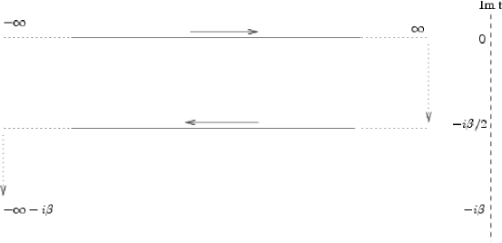
Figure 1.1: Integration path in TFD. The fields that “live” in the imaginary time $x_{0}-i\beta/2$ are called Thermal Ghosts.

If we take the limit $\tau\rightarrow\infty$, the fields will be split into two regions; the “real” fields that live on the real axis of time, and the so called thermal ghosts. This means that the Fock-space is duplicated [UMT82]. This formalism is named Thermo-Field Dynamics (TFD). The formal algebraic formulation of TFD was proposed by [Oji81]. The path integral formulation for the fermion fields, and the real-time Feynman rules for gauge theories with fermions, at finite temperature and density, were developed by [KSW85] and [NS84, MOU84].

One of the consequences of the appearance of thermal ghosts is that we will get four two-point propagators instead of one for each field, i.e., if we denote by $\phi_{1}=\phi(x)$ the real field and by $\phi_{2}=\phi(x_{0}-i\beta/2,\bm{p})$ the ghost fields, we have

$$D_{T_{ij}}(x,y;T)=\langle\!\langle 0|T\phi_{i}(x)\phi_{j}(y)|0\rangle\!\rangle,$$ (1.52)

where by $|0\rangle\!\rangle$ we understand the thermal vacuum state or “populated” vacuum state, and the propagator with the real fields $D_{Th_{11}}$ is the so-called Dolan-Jackiw propagator (DJp) [DJ74].

The prescriptions for loop calculations are:

• The thermal insertions appear only through loop calculations.

• Thermal ghosts must be included in calculations at two or more loops

Since in this work we will deal only with one-loop corrections, we need only to consider the DJp. I will not discuss the construction of the DJp, which isbased on the KMS boundary conditions indicated in eq.1.51 and the time-order of the fields along the path described in Fig.1.1. A general formula for the DJp for bosonic fields is

$$D_{DJ}(p) = \int\frac{dk_{0}}{2\pi i}\lim_{\eta\to 0}\left[\frac{D(k_{0}+i\eta,\bm{p})-D(k_{0}-i\eta,\bm{p})}{k_{0}-p_{0}-i\epsilon}\right]$$ (1.53)

$$\quad+n_{B}(p_{0})\big{[}D(p_{0}+i\epsilon,\bm{p})-D(p_{0}-i\epsilon,\bm{p})\big{]},$$

where $-iD$ is the free propagator in momentum space defined in equation (1.38) and $n_{B}$ is the Bose-Einstein distribution defined as

$$n_{B}(x)=\frac{1}{e^{\beta x}-1}.$$ (1.54)

For a free propagator of the form

$$iD^{-1}(p)=p^{2}-2ap_{0}-b,$$ (1.55)

the corresponding DJp, following eq.1.53 is

$$D_{DJ}(p)=\frac{i}{p^{2}-2ap_{0}-b+i\epsilon}+2\pi n_{B}(|p_{0}|)\delta(p^{2}-2ap_{0}-b).$$ (1.56)

To distinguish the propagator at zero temperature and the pure thermal part of the DJp, we will refer to them as the free-propagator and the thermal insertion, respectively.

1.2.2 Covariant formalism and finite chemical potential

Consider the case of a fermionic field within a dense medium, asymmetric with respect to baryon number. If the baryon number density is $n=\psi^{\dagger}\psi$, the introduction of a chemical potential into the Lagrangian density as a Lagrange multiplier of this conserved quantity gives

$${\cal L}+\mu n = \bar{\psi}(i\gamma\partial-m)\psi+\mu\psi^{\dagger}\psi=\bar{\psi}(i\gamma\partial+\gamma_{0}\mu-m)\psi$$ (1.57)

$$= \bar{\psi}(i\gamma^{\mu}[\partial_{\mu}-i\mu\delta_{\mu 0}]-m)\psi.$$

This means that the chemical potential acts like a gauge field [Wel82, Act85]. The corresponding propagator is

$$S_{F}(p)=\frac{i(\gamma p+\gamma_{0}\mu+m)}{(p_{0}+\mu)^{2}-\bm{p}^{2}-m^{2}+i\epsilon}.$$ (1.58)

The presence of a thermal bath breaks Lorentz invariance, since it plays the role of a privileged reference frame. Nevertheless, formally we can “restore” the Lorentz symmetry in such a way that it is possible to give a covariant form to the equations, through the introduction of the fourt-velocity $u_{\mu}$ between the observer and the thermal bath [Wel82]. In the rest frame (i.e. where the thermal bath is at rest with respect the observer), we have

$$u=(1,0,0,0).$$ (1.59)

Although this work is performed in the rest frame, we use the symbol $u_{\mu}=\delta_{\mu 0}$ recalling that in principle it is possible to use a covariant formalism.

1.2.3 QCD at finite isospin chemical potential

As was indicated in the previous section, the chemical potential in eq.(1.50) is added to the Lagrangian as a Lagrange multiplier of a conserved charge. In this thesis we will consider the isospin chemical potential related to the isospin number, which indicates the difference of the baryon number between the $u$ and the $d$ fields. The isospin density number operator is defined as

$$n_{I}\equiv{\textstyle\frac{1}{2}}(u^{\dagger}u-d^{\dagger}d)=q^{\dagger}\frac{\tau_{3}}{2}q$$ (1.60)

where $q=(u,d)$ in the case of two flavors. Then the QCD-Lagrangian with massive quarks acquires the form

$${\cal L}_{QCD}(M,0,0,0)+\mu_{\mbox{\tiny I}}n_{I} = {\cal L}^{0}_{QCD}+{\cal L}_{QCD}^{A}-\bar{q}Mq+\mu_{\mbox{\tiny I}}\bar{q}\gamma\cdot u\frac{\tau_{3}}{2}q$$ (1.61)

$$= {\cal L}_{QCD}(M,0,{\textstyle\frac{1}{2}}\mu_{\mbox{\tiny I}}\tau_{3}u,0).$$

Chapter 2 Tree-level masses, thermal propagators and vertices at finite isospin chemical potential.

For radiative calculations, we need the different propagators derived from the free Lagrangian. To obtain the effective Lagrangian at the one-loop level, first we have to calculate the vacuum expectation value of the field $U$, named $\bar{U}$. Taking the ${\cal O}(P^{2})$ Lagrangian and setting $\pi^{a}=0$ we have that the effective potential is

$$V_{eff}=-\frac{f^{2}}{4}Tr\left[\mu_{\mbox{\tiny I}}^{2}\left[{\textstyle\frac{1}{2}}\tau_{3},\bar{U}\right]\left[{\textstyle\frac{1}{2}}\tau_{3},\bar{U}^{\dagger}\right]+2BM\left(\bar{U}+\bar{U}^{\dagger}\right)\right].$$ (2.1)

Taking the general expression for $\bar{U}$

$$\bar{U}=\cos\varphi+i\bm{\tau}\cdot\bm{n}\sin\varphi,$$ (2.2)

with

$$\bm{n}=\cos\phi\sin\theta\bm{e_{1}}+\sin\phi\sin\theta\bm{e_{2}}+\cos\theta\bm{e_{3}},$$ (2.3)

the previous expression becomes

$$V_{eff}=-f^{2}\left({\textstyle\frac{1}{2}}\mu_{\mbox{\tiny I}}^{2}\sin^{2}\varphi\sin\theta-m^{2}\cos\varphi\right).$$ (2.4)

Minimizing the effective potential, we find that the vacuum expectation value of the $U$ fields depends on $\mu_{\mbox{\tiny I}}$ [KST⁺00, KT01] and is given by

$$\bar{U}=\left\{\begin{array}[]{cl}1&\quad\mbox{if}\quad\mu_{\mbox{\tiny I}}^{2}<m^{2}\\ \frac{m^{2}}{\mu_{\mbox{\tiny I}}^{2}}+i[\tau_{1}\cos\phi+\tau_{2}\sin\phi]\sqrt{1-{\textstyle\frac{m^{4}}{\mu_{\mbox{\tiny I}}^{4}}}}&\quad\mbox{if}\quad\mu_{\mbox{\tiny I}}^{2}>m^{2}\end{array}\right.$$ (2.5)

Now, we can expand the chiral Lagrangian in terms of the pion degrees of freedom up to the necessary powers for one-loop radiative corrections. The two phases, $|\mu_{\mbox{\tiny I}}|<m$ and $|\mu_{\mbox{\tiny I}}|>m$, will be referred to as the first phase and the second phase, respectively. The expansion of the chiral Lagrangian is explained in App. A.1.

2.1 First phase

For the case of the first phase, the relevant Lagrangian for one-loop corrections is ${\cal L}_{1-loop}={\cal L}_{2,2}+{\cal L}_{2,4}+{\cal L}_{4,2}$ as was indicated in Eq. (1.34), where the ${\cal L}_{i,j}$ terms are

$${\cal L}_{2,2} = \frac{1}{2}\left[\left(\partial\pi_{0}\right)^{2}-m^{2}\pi_{0}^{2}\right]+\left|\partial_{I}\pi\right|^{2}-m^{2}\left|\pi\right|^{2}$$ (2.6)

$${\cal L}_{2,4} = \frac{1}{4!}\frac{m^{2}}{f^{2}}\pi_{0}^{4}+\frac{1}{6f^{2}}\left[-4\left|\partial_{I}\pi\right|^{2}\left|\pi\right|^{2}+\left(\partial\left|\pi\right|^{2}\right)^{2}+m^{2}\left(\left|\pi\right|^{2}\right)^{2}\right]$$ (2.7)

$$+\frac{1}{6f^{2}}\left[-2\left|\partial_{I}\pi\right|^{2}\pi_{0}^{2}-2\left(\partial\pi_{0}\right)^{2}\left|\pi\right|^{2}+\partial\pi_{0}^{2}\cdot\partial\left|\pi\right|^{2}+m^{2}\pi_{0}^{2}\left|\pi\right|^{2}\right]$$

$${\cal L}_{4,2} = \frac{m^{2}}{f^{2}}\left[2l_{4}\left|\partial_{I}\pi\right|^{2}-2m^{2}(l_{3}+l_{4})\left|\pi\right|^{2}+l_{4}\left(\partial\pi_{0}\right)^{2}-m^{2}(l_{3}+l_{4}-\epsilon_{ud}^{2}l_{7})\pi_{0}^{2}\right],$$

using the standard definition of the pion fields

$$\pi_{0}=\pi_{3},\qquad\pi_{\pm}={\textstyle\frac{1}{\sqrt{2}}}(\pi_{1}\mp i\pi_{2}).$$ (2.9)

In the previous expressions

$$|\pi|^{2}\equiv\pi^{+}\pi^{-},\qquad|\partial_{I}\pi|^{2}=(\partial_{I}^{+}\pi^{+})(\partial_{I}^{-}\pi^{-}),$$ (2.10)

and the derivative $\partial_{I\pm}$ that appears in the Lagrangian is defined as

$$\partial_{I}^{\pm}\equiv\partial\mp i\mu_{I}u.$$ (2.11)

This definition of the covariant derivative is natural, since we know [Act85] that the chemical potential is introduced as the zero component of an external “gauge” field. The term $\epsilon_{ud}$ in Eq. LABEL:L_42_phase1 is the quark masses ratio $(m_{u}-m_{d})/(m_{u}+m_{d})$.

To obtain the DJp, first consider the equations of motion in momentum space, extracted from the free Lagrangian ${\cal L}_{2,2}$ in Eq. (2.6).

$$i\bm{D}^{-1}=i\left(\begin{array}[]{ccc}D^{-1}_{\mbox{\tiny$00$}}&0&0\\ 0&0&D^{-1}_{\mbox{\tiny$+-$}}\\ 0&D^{-1}_{\mbox{\tiny$-+$}}&0\end{array}\right)$$ (2.12)

The non-zero elements of the free propagator matrix are

$$iD^{-1}(p)_{\mbox{\tiny$00$}} = p^{2}-m^{2}$$ (2.13)

$$iD^{-1}(p)_{\mbox{\tiny$+-$}} = (p-\mu_{\mbox{\tiny I}}u)^{2}-m^{2}$$ (2.14)

$$iD^{-1}(p)_{\mbox{\tiny$-+$}} = iD^{-1}(-p)_{\mbox{\tiny$+-$}}.$$ (2.15)

It is easy to derive the tree-level masses, because the propagator matrix has no crossed terms. Then, the equations of motion act independently on each pion field. The previous equations are the equations of motion in momentum space $iD^{-1}(p)_{ij}$ respect to the field $\pi_{j}$. From these equations, it is easy to associate the different tree-level masses, obtaining

$$m_{0}=m,\qquad\qquad m_{\pm}=m\mp\mu_{\mbox{\tiny I}},$$ (2.16)

where the the different pion masses are defined as their rest energy.

Since our calculation will be at the one-loop level, we do not need, as was said previously, the full formalism of thermo field dynamics including thermal ghosts. Then, by the general formula in Eq. (1.53), the DJp are

$$D_{DJ}(p)_{\mbox{\tiny$00$}} = \frac{i}{p^{2}-m^{2}+i\epsilon}+2\pi n_{B}(|p_{0}|)\delta(p^{2}-m^{2})$$ (2.17)

$$D_{DJ}(p)_{\mbox{\tiny$+-$}} = \frac{i}{(p+\mu_{\mbox{\tiny I}}u)^{2}-m^{2}+i\epsilon}+2\pi n_{B}(|p_{0}|)\delta\big{(}(p+\mu_{\mbox{\tiny I}}u)^{2}-m^{2}\big{)}$$ (2.18)

$$D_{DJ}(p)_{\mbox{\tiny$-+$}} = D_{\mbox{\tiny$+-$}}(-p;T).$$ (2.19)

Diagrammatically, the neutral pion propagator will be denoted as a double line. The $\pm$ propagator will be denoted as a single line with an arrow pointing in direction from $+$ to $-$, as is indicated in Fig. 2.1.

Figure 2.1: Propagators in the first phase (and in second phase for $|\mu_{\mbox{\tiny I}}|\gtrsim m$). The double line denotes the neutral propagator. The single line denotes the charged propagator with an arrow pointing from $+$ to $-$.

The vertices extracted from ${\cal L}_{2,4}$ and ${\cal L}_{4,2}$, shown in eqs. (2.7) and (LABEL:L_42_phase1), are

$$V_{2,4}^{\mbox{\tiny$0000$}} = i\frac{m^{2}}{f^{2}}$$ (2.20)

$$V_{2,4}^{\mbox{\tiny$00\pm$}} = \frac{i}{3f^{2}}\Big{\{}2pq+2p_{\mbox{\tiny$+$}}p_{\mbox{\tiny$-$}}-\big{[}p+q\big{]}\big{[}p_{\mbox{\tiny$+$}}+p_{\mbox{\tiny$-$}}\big{]}-\mu_{\mbox{\tiny I}}\big{[}p_{\mbox{\tiny$+$}}^{0}-p_{\mbox{\tiny$-$}}^{0}\big{]}+m^{2}-2\mu_{\mbox{\tiny I}}^{2}\Big{\}}$$

$$V_{2,4}^{{\mbox{\tiny$\pm\pm$}}} = \frac{i}{3f^{2}}\Big{\{}-2p_{\mbox{\tiny$+$}}q_{\mbox{\tiny$+$}}-2p_{\mbox{\tiny$-$}}q_{\mbox{\tiny$-$}}+\big{[}p_{\mbox{\tiny$+$}}+q_{\mbox{\tiny$+$}}\big{]}\big{[}p_{\mbox{\tiny$-$}}+q_{\mbox{\tiny$-$}}\big{]}$$ (2.22)

$$\hskip 28.45274pt+4\mu_{\mbox{\tiny I}}\big{[}p_{\mbox{\tiny$+$}}^{0}+q_{\mbox{\tiny$+$}}^{0}-p_{\mbox{\tiny$-$}}^{0}-q_{\mbox{\tiny$-$}}^{0}\big{]}+2m^{2}-8\mu_{\mbox{\tiny I}}^{2}\Big{\}}$$

$$V_{4,2}^{{\mbox{\tiny$00$}}} = -2i\frac{m^{2}}{f^{2}}\big{[}2pql_{4}+m^{2}(l_{3}+l_{4}-{\epsilon_{ud}}^{2}l_{7})\big{]}$$ (2.23)

$$V_{4,2}^{{\mbox{\tiny$-+$}}} = 2i\frac{m^{2}}{f^{2}}\Big{\{}\big{[}-p_{\mbox{\tiny$+$}}p_{\mbox{\tiny$-$}}+\mu_{\mbox{\tiny I}}(p_{\mbox{\tiny$+$}}^{0}-p_{\mbox{\tiny$-$}}^{0})+\mu_{\mbox{\tiny I}}^{2}\big{]}l_{4}-m^{2}(l_{3}+l_{4})\Big{\}},$$ (2.24)

where $p$ and $q$ denote the external momentum of the $\pi^{0}$ legs and $p_{\pm}$ and $q_{\pm}$ denote the external momenta of the $\pi^{\pm}$ legs. In all cases, the momentum emerges from the vertex.

Diagrammatically, using the convention for the propagators, a double line will denote a neutral pion leg and a single line a charged pions, where an arrow pointing away from the vertex denotes a $\pi^{+}$ leg, and an arrow pointing into the vertex denotes a $\pi^{-}$, as can be seen in Fig. 2.2.

Figure 2.2: Vertices in the first phase (and in second phase for $|\mu_{\mbox{\tiny I}}|\gtrsim m$). The double line denotes the neutral pion leg. The single line represents the charged pion leg with an arrow pointing outside from the vertex for the $\pi^{+}$ and into the vertex for the $\pi^{-}$ (or $\tilde{\pi}^{+}$ and $\tilde{\pi}^{-}$ in second phase for $|\mu_{\mbox{\tiny I}}|\gtrsim m$)

2.2 Second phase

Let us denote the vacuum expectation value of the $U$ field as

$$\bar{U}=c+i\tilde{\tau}_{1}s,$$ (2.25)

with

$$c\equiv\frac{m^{2}}{\mu_{\mbox{\tiny I}}^{2}},\qquad s\equiv\sqrt{1-\frac{m^{4}}{\mu_{\mbox{\tiny I}}^{4}}},$$ (2.26)

where, for any vector, the $\tilde{\mbox{v}}_{i}$ components refer to the components of a rotated vector by the azimuthal angle $\phi$:

$$\tilde{\mbox{v}}_{1}=\mbox{v}_{1}\cos\phi+\mbox{v}_{2}\sin\phi,\qquad\tilde{\mbox{v}}_{2}=-\mbox{v}_{1}\sin\phi+\mbox{v}_{2}\cos\phi,\qquad\tilde{\mbox{v}}_{3}=\mbox{v}_{3}.$$ (2.27)

The vacuum expectation value of the $U$ fields breaks SU(2)$\rightarrow$U(1).

The expanded Lagrangian, keeping all the details, is given by

$${\cal L}_{2,2} = {\textstyle\frac{1}{2}}(\partial\bm{\pi})^{2}-{\textstyle\frac{1}{2}}\mu_{\mbox{\tiny$I$}}^{2}(s^{2}\tilde{\pi}_{{\mbox{\tiny$1$}}}^{2}+\pi_{{\mbox{\tiny$3$}}}^{2})-|\mu_{\mbox{\tiny$I$}}|c(\tilde{\pi}_{{\mbox{\tiny$1$}}}\partial_{{\mbox{\tiny$0$}}}\tilde{\pi}_{{\mbox{\tiny$2$}}}-\tilde{\pi}_{{\mbox{\tiny$2$}}}\partial_{{\mbox{\tiny$0$}}}\tilde{\pi}_{{\mbox{\tiny$1$}}})$$ (2.28)

$${\cal L}_{2,3} = \frac{1}{f}|\mu_{\mbox{\tiny$I$}}|s\big{[}(\tilde{\pi}_{{\mbox{\tiny$1$}}}^{2}+\pi_{{\mbox{\tiny$3$}}}^{2})\partial_{{\mbox{\tiny$0$}}}\tilde{\pi}_{{\mbox{\tiny$2$}}}-{\textstyle\frac{1}{2}}|\mu_{\mbox{\tiny$I$}}|c\tilde{\pi}_{{\mbox{\tiny$1$}}}\bm{\pi}^{2}\big{]}$$ (2.29)

$${\cal L}_{2,4} = \frac{1}{6f^{2}}\Big{\{}\big{[}-(\partial\bm{\pi})^{2}+\mu_{\mbox{\tiny$I$}}^{2}(s^{2}\tilde{\pi}_{{\mbox{\tiny$1$}}}^{2}+\pi_{{\mbox{\tiny$3$}}}^{2}-{\textstyle\frac{3}{4}}c^{2}\bm{\pi}^{2})$$ (2.30)

$$\hskip 85.35826pt+2|\mu_{\mbox{\tiny I}}|c(\tilde{\pi}_{{\mbox{\tiny$1$}}}\partial_{{\mbox{\tiny$0$}}}\tilde{\pi}_{{\mbox{\tiny$2$}}}-\tilde{\pi}_{{\mbox{\tiny$2$}}}\partial_{{\mbox{\tiny$0$}}}\tilde{\pi}_{{\mbox{\tiny$1$}}})\big{]}\bm{\pi}^{2}+(\bm{\pi}\cdot\partial\bm{\pi})^{2}\Big{\}}$$

$${\cal L}_{4,1} = \frac{1}{f}\mu_{\mbox{\tiny$I$}}^{4}cs[4s^{2}(l_{1}+l_{2})-2c^{2}l_{3}-s^{2}l_{4}]\tilde{\pi}_{{\mbox{\tiny$1$}}}$$ (2.31)

$${\cal L}_{4,2} = \frac{1}{f^{2}}\mu_{\mbox{\tiny$I$}}^{2}\Big{\{}2s^{2}\big{[}(\partial\bm{\pi})^{2}+2(\partial_{{\mbox{\tiny$0$}}}\tilde{\pi}_{{\mbox{\tiny$2$}}})^{2}\big{]}l_{1}+2s^{2}\big{[}(\partial_{{\mbox{\tiny$0$}}}\bm{\pi})^{2}+(\partial\tilde{\pi}_{{\mbox{\tiny$2$}}})^{2}+(\partial_{{\mbox{\tiny$0$}}}\tilde{\pi}_{{\mbox{\tiny$2$}}})^{2}\big{]}l_{2}$$

$$\qquad-2s^{2}\big{[}8|\mu_{\mbox{\tiny$I$}}|c\tilde{\pi}_{{\mbox{\tiny$1$}}}\partial_{0}\tilde{\pi}_{{\mbox{\tiny$2$}}}+\mu_{\mbox{\tiny$I$}}^{2}(s^{2}\bm{\pi}^{2}-3c^{2}\tilde{\pi}_{{\mbox{\tiny$1$}}}^{2}-\tilde{\pi}_{{\mbox{\tiny$2$}}}^{2})\big{]}(l_{1}+l_{2})$$

$$\qquad+\mu_{\mbox{\tiny$I$}}^{2}c^{2}\big{[}s^{2}\tilde{\pi}_{{\mbox{\tiny$1$}}}^{2}-c^{2}\bm{\pi}^{2}\big{]}l_{3}+\big{[}c^{2}(\partial\bm{\pi})^{2}+2|\mu_{\mbox{\tiny$I$}}|c(1-3c^{2})\tilde{\pi}_{{\mbox{\tiny$1$}}}\partial_{{\mbox{\tiny$0$}}}\tilde{\pi}_{{\mbox{\tiny$2$}}}$$

$$\quad\qquad-\mu_{\mbox{\tiny I}}^{2}c^{2}\{(s^{2}+1)\bm{\pi}^{2}-(c^{2}-s^{2})\tilde{\pi}_{{\mbox{\tiny$1$}}}^{2}-\tilde{\pi}_{{\mbox{\tiny$2$}}}^{2}\}\big{]}l_{4}+\mu_{\mbox{\tiny$I$}}^{2}c^{2}\epsilon_{{\mbox{\tiny$ud$}}}^{2}\pi_{3}^{2}l_{7}\Big{\}}.$$

Here, $m^{2}=\mu_{\mbox{\tiny I}}^{2}c$ for further considerations, and I will consider a negative chemical potential ($\mu_{\mbox{\tiny$I$}}=-|\mu_{\mbox{\tiny$I$}}|$) as is the case in neutron stars, where a condensate of $\pi_{-}$ quasi-particles might exist [YP04]. The same happens for the $\pi_{+}$, for the opposite sign of $\mu_{\mbox{\tiny$I$}}$. Note that, in the second phase, there vertices with three legs will appear from (${\cal L}_{2,3}$), and with one leg from (${\cal L}_{4,1}$). The latter is responsible for the counter-terms of the tadpoles, but they will not be considered in the approximation we will use next.

The inverse of the free propagator for pions in momentum space, i.e., the kernel of equations of motion extracted from ${\cal L}_{2,2}$ is given by the matrix

$$i\bm{D}^{-1}=i\left(\begin{array}[]{ccc}D^{-1}_{\mbox{\tiny$11$}}&D^{-1}_{\mbox{\tiny$12$}}&0\\ D^{-1}_{\mbox{\tiny$21$}}&D^{-1}_{\mbox{\tiny$22$}}&0\\ 0&0&D^{-1}_{\mbox{\tiny$33$}}\end{array}\right)=\left(\begin{array}[]{ccc}p^{2}-\mu_{\mbox{\tiny$I$}}^{2}s^{2}&2i|\mu_{\mbox{\tiny$I$}}|cp_{0}&0\\ -2i|\mu_{\mbox{\tiny$I$}}|cp_{0}&p^{2}&0\\ 0&0&p^{2}-\mu_{\mbox{\tiny$I$}}^{2}\end{array}\right)$$ (2.33)

To extract the tree-level masses, we calculate the poles of the determinant of $D$ at zero momentum as is prescribed in [KT01]

$$\left|i\bm{D}^{-1}(p)\right|_{\bm{p}=0}=\big{[}p_{0}^{2}-\mu_{\mbox{\tiny I}}^{2}\big{]}\big{[}p_{0}^{2}-\mu_{\mbox{\tiny I}}^{2}(1+3c^{2})\big{]}p_{0}^{2}=0.$$ (2.34)

We can identify the masses with respect to the results in Eq. (2.16), which have to match for $\mu_{\mbox{\tiny I}}=m$. Then, the tree-level masses for the second phase are

$$m_{0}=|\mu_{\mbox{\tiny I}}|,\qquad m_{+}=|\mu_{\mbox{\tiny I}}|\sqrt{1+3c^{2}},\qquad m_{-}=0.$$ (2.35)

In Figure 2.3, we can see the behavior of the masses at tree-level in both phases as a function of a negative chemical potential (see also [SS01] for the treatment at tree-level).

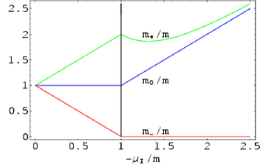
Figure 2.3: Pion masses as a function of the isospin chemical potential at tree-level

We can identify the $\pi_{3}=\pi_{0}$ field, as in [KT01], through its mass at $|\mu_{\mbox{\tiny I}}|=m$ and because it is diagonal in the propagator matrix. Therefore, there will be no difficulties in handling this propagator,

$$D_{DJ}(p)_{\mbox{\tiny$00$}}=\frac{i}{p^{2}-\mu_{\mbox{\tiny I}}^{2}+i\epsilon}+2\pi n_{B}(p_{0})\delta(p^{2}-\mu_{\mbox{\tiny I}}^{2}).$$ (2.36)

Unfortunately, this is not the case for the charged pions, which are mixed in a non-trivial way.

The free propagator for the charged pions in momentum space is

$$\tilde{\bm{D}}=\frac{i}{[p^{4}-p^{2}\mu_{\mbox{\tiny I}}^{2}s^{2}-4\mu_{\mbox{\tiny I}}^{2}c^{2}p_{0}^{2}]}\left(\begin{array}[]{cc}p^{2}&-2i|\mu_{\mbox{\tiny I}}|cp_{0}\\ 2i|\mu_{\mbox{\tiny I}}|cp_{0}&p^{2}-\mu_{\mbox{\tiny I}}^{2}s^{2}\\ \end{array}\right)$$ (2.37)

with $\tilde{\bm{D}}_{ij}\equiv\bm{D}_{ij\neq 3}$. The Dolan-Jackiw propagators can be constructed with the general formula indicated in Eq. (1.53).

The main difficulty with this matrix propagator is that it is very cumbersome to use it in the different loop corrections. This fact motivates to proceed in a systematic way, through an expansion in a new appropriate smallness parameter, namely $s$ when $|\mu_{\mbox{\tiny I}}|\gtrsim m$ or $c$ when $|\mu_{\mbox{\tiny I}}|\gg m$.

It is not difficult to realize that the different vertices that appear in our Lagrangian will correspond to different powers of $c$ or $s$, depending on the case. Although it could appear as a trivial correction, we will keep only the zeroth order in all calculations. As we will see, this procedure is not trivial at all and provides us with interesting information about the behavior of the pion masses as function of temperature and isospin chemical potential.

If we scale all the parameters with $|\mu_{\mbox{\tiny$I$}}|$ in all structures needed for one-loop corrections, we have that:

Propagators $$\rightarrow D(p;T,\mu_{\mbox{\tiny$I$}};m)=\frac{1}{\mu_{\mbox{\tiny$I$}}^{2}}\bar{\bm{D}}(\bar{p};\bar{T},c)$$ (2.38)

$$l_{i}~{}\textrm{constants} \rightarrow l_{i}(\Lambda)=\frac{\gamma_{i}}{32\pi^{2}}\left[\bar{l}_{i}-\lambda-\ln(c\bar{\Lambda}^{2})\right]$$ (2.39)

Vertices $$\rightarrow V_{n,m}(p;\mu_{\mbox{\tiny$I$}};f,m,\Lambda)=\frac{|\mu_{\mbox{\tiny$I$}}|^{n}}{f^{m+n-4}}v_{n,m}(\bar{p};\bar{\Lambda},c)$$ (2.40)

Integrals $$\rightarrow \int\frac{d^{d}k}{(2\pi)^{d}}\Lambda^{4-d}=\mu_{\mbox{\tiny$I$}}^{4}\int\frac{d^{d}\bar{k}}{(2\pi)^{d}}\bar{\Lambda}^{4-d}$$ (2.41)

Corrections $$\rightarrow \Sigma(p_{0};T,\mu_{\mbox{\tiny$I$}};f,m,\Lambda)=\frac{\mu_{\mbox{\tiny I}}^{4}}{(4\pi f)^{2}}\sigma(\bar{p}_{0};\bar{T},c;\bar{\Lambda})$$ (2.42)

where from now on the bar on a parameter means that it is scaled with $|\mu_{\mbox{\tiny$I$}}|$. It is possible then to expand the propagator in powers of $s^{n}$ for$|\mu_{\mbox{\tiny$I$}}|\gtrsim m$ and $c^{n}$ when $|\mu_{\mbox{\tiny$I$}}|\gg m$. Doing the same with the vertices, the resulting radiative corrections will be expressed in powers of $s$ and $c$. The problem with divergences is then also fixed since they appear in powers of $c$ and $s$.

As we said before, we will keep only the $n=0$ terms in the previous expansions. This approximation is non-trivial, since it allows us to explore the behavior of the renormalized masses precisely in the vicinity of the transition point and also in the region of high values of the chemical potential. Further corrections could also be calculated, taking into account higher order vertices and propagators.

We will avoid the region where $c\sim s$ (i.e. arround $c=s=\frac{1}{\sqrt{2}}$) and consider only the region where $c\rightarrow 0$ or $s\rightarrow 0$. This excluded area becomes smaller when $n$ (the order of the expansion) starts to grow. By demanding that $c^{n+1},s^{n+1}\lesssim\frac{1}{2}(\frac{1}{\sqrt{2}})^{n+1}$, we achieve this condition. Note that if $n=0$, we would exclude the region of the chemical potential where $\sqrt{\frac{8}{7}}m^{2}\lesssim\mu_{\mbox{\tiny I}}^{2}\lesssim\sqrt{8}m^{2}$. We remark again that by going to higher orders in our expansion, the excluded region becomes smaller, so this is the best bound.

2.2.1 Propagators and vertices at order $s^{0}$

As was said before, the neutral pion propagator is diagonal with respect to the charged ones. Its propagator will be the same in both limits at any order.

The propagator for the charged pions at ${\cal O}(s^{0})$ is given by

$$\tilde{\bm{D}}=\frac{i}{[p^{4}-4\mu_{\mbox{\tiny$I$}}^{2}p_{0}^{2}]}\left(\begin{array}[]{cc}p^{2}&-2i|\mu_{\mbox{\tiny$I$}}|p_{0}\\ 2i|\mu_{\mbox{\tiny$I$}}|p_{0}&p^{2}\\ \end{array}\right)+\frac{1}{\mu_{\mbox{\tiny$I$}}^{2}}{\cal O}(s^{2})$$ (2.43)

It is more convenient to work with the combination of fields

$$\tilde{\pi}_{\pm}={\textstyle\frac{1}{\sqrt{2}}}(\tilde{\pi}_{{\mbox{\tiny$1$}}}\mp i\tilde{\pi}_{{\mbox{\tiny$2$}}}),$$ (2.44)

where the tilde tilde convention was described in equation (2.27) We remark that the $\tilde{\pi}_{\pm}$ fields do not correspond to the physical charged pion fields but to a combination of them. This fact is a consequence of the non-trivial vacuum structure in this phase. This combination is also not trivial due to derivative terms and the inverse D’Alembertian operator. I would like to mention that, in the first phase ($\mu_{\mbox{\tiny I}}<m$), the $\pi_{\pm}$ correspond effectively to the charged pions and the propagator becomes anti-diagonal. Then, the inverse propagator for charged pions are

$$i\tilde{\bm{D}}^{-1}=i\left(\begin{array}[]{cc}D^{-1}_{\mbox{\tiny$++$}}&D^{-1}_{\mbox{\tiny$+-$}}\\ &\\ D^{-1}_{\mbox{\tiny$-+$}}&D^{-1}_{\mbox{\tiny$--$}}\end{array}\right)=\left(\begin{array}[]{cc}-{\textstyle\frac{1}{2}}\mu_{\mbox{\tiny$I$}}^{2}s^{2}&p^{2}+2|\mu_{\mbox{\tiny$I$}}|cp_{0}-{\textstyle\frac{1}{2}}\mu_{\mbox{\tiny$I$}}^{2}s^{2}\\ &\\ p^{2}-2|\mu_{\mbox{\tiny$I$}}|cp_{0}-{\textstyle\frac{1}{2}}\mu_{\mbox{\tiny$I$}}^{2}s^{2}&-{\textstyle\frac{1}{2}}\mu_{\mbox{\tiny$I$}}^{2}s^{2}\end{array}\right)$$ (2.45)

and the free propagator matrix is

$$\tilde{\bm{D}}=i\left(\begin{array}[]{cc}0&\frac{1}{p^{2}-2|\mu_{\mbox{\tiny$I$}}|p_{0}}\\ \frac{1}{p^{2}+2|\mu_{\mbox{\tiny$I$}}|p_{0}}&0\\ \end{array}\right)+\frac{1}{\mu_{\mbox{\tiny$I$}}^{2}}{\cal O}(s).$$ (2.46)

The Dolan-Jackiw propagators for charged pions, including isospin chemical potential (enough for one-loop calculations), are

$$D_{DJ}(p)_{{\mbox{\tiny$+-$}}} = \frac{i}{p^{2}-2|\mu_{\mbox{\tiny$I$}}|p_{0}+i\epsilon}+2\pi n_{B}(|p_{0}|)\delta(p^{2}-2|\mu_{\mbox{\tiny$I$}}|p_{0})+\frac{1}{\mu_{\mbox{\tiny$I$}}^{2}}{\cal O}(s^{2}),$$ (2.47)

$$D_{DJ}(p)_{\mbox{\tiny$-+$}} = D_{DJ}(-p)_{\mbox{\tiny$+-$}},$$ (2.48)

and the other propagators, $\bar{D}_{\mbox{\tiny$++$}}$ and $\bar{D}_{\mbox{\tiny$--$}}$ are of order $s^{2}$, so we will neglect them. Diagrammatically, the propagators in this limit are the same as in the first phase (see Fig. 2.1). Note that, in the case where $|\mu_{\mbox{\tiny I}}|=m$, the fields $\tilde{\pi}^{\pm}$ can be identified as the physical fields $\pi^{\pm}$.

The relevant vertices at order $s^{0}$ are

$$V_{2,4}^{\mbox{\tiny$0000$}} = i\frac{\mu_{\mbox{\tiny I}}^{2}}{f^{2}}$$ (2.49)

$$V_{2,4}^{\mbox{\tiny$00+-$}} = \frac{i}{3f^{2}}\Big{\{}2pq+2p_{\mbox{\tiny$+$}}p_{\mbox{\tiny$-$}}-\big{[}p+q\big{]}\big{[}p_{\mbox{\tiny$+$}}+p_{\mbox{\tiny$-$}}\big{]}+|\mu_{\mbox{\tiny I}}|\big{[}p_{\mbox{\tiny$+$}}^{0}-p_{\mbox{\tiny$-$}}^{0}\big{]}-\mu_{\mbox{\tiny I}}^{2}\Big{\}}$$ (2.50)

$$V_{2,4}^{{\mbox{\tiny$++--$}}} = \frac{i}{3f^{2}}\Big{\{}-2p_{\mbox{\tiny$+$}}q_{\mbox{\tiny$+$}}-2p_{\mbox{\tiny$-$}}q_{\mbox{\tiny$-$}}+\big{[}p_{\mbox{\tiny$+$}}+q_{\mbox{\tiny$+$}}\big{]}\big{[}p_{\mbox{\tiny$-$}}+q_{\mbox{\tiny$-$}}\big{]}$$ (2.51)

$$\hskip 56.9055pt-4|\mu_{\mbox{\tiny I}}|\big{[}p_{\mbox{\tiny$+$}}^{0}+q_{\mbox{\tiny$+$}}^{0}-p_{\mbox{\tiny$-$}}^{0}-q_{\mbox{\tiny$-$}}^{0}\big{]}-6\mu_{\mbox{\tiny I}}^{2}\Big{\}}$$

$$V_{4,2}^{{\mbox{\tiny$00$}}} = -2i\frac{\mu_{\mbox{\tiny I}}^{2}}{f^{2}}\Big{\{}2pql_{4}+\mu_{\mbox{\tiny I}}^{2}(l_{3}+l_{4}-{\epsilon_{ud}}^{2}l_{7})\Big{\}}$$ (2.52)

$$V_{4,2}^{{\mbox{\tiny$-+$}}} = -2i\frac{\mu_{\mbox{\tiny I}}^{2}}{f^{2}}\Big{\{}\big{[}p_{\mbox{\tiny$+$}}p_{\mbox{\tiny$-$}}+|\mu_{\mbox{\tiny I}}|(p_{\mbox{\tiny$+$}}^{0}-p_{\mbox{\tiny$-$}}^{0})]l_{4}+\mu_{\mbox{\tiny I}}^{2}l_{3}\Big{\}},$$ (2.53)

which, diagrammatically, are the same as the first phase (Fig. 2.2), where $p$ and $q$ denote the external momenta of $\pi^{0}$ legs and $p_{\pm}$ and $q_{\pm}$ denote the external momenta of the $\pi^{\pm}$ leg. In all cases, the momentum emerges from the vertex. These vertices include higher terms of order $s$ and $s^{2}$, and other vertices also appear: $v_{2,2}^{{\mbox{\tiny$\pm\pm$}}}$, $v_{2,4}^{{\mbox{\tiny$00\pm\pm$}}}$, $v_{2,4}^{{\mbox{\tiny$\mp\pm\pm\pm$}}}$ of ${\cal O}(s^{2})$ and $v_{2,3}^{\mbox{\tiny$\mp\pm\pm$}}$,$v_{2,3}^{\mbox{\tiny$00\pm$}}$, $v_{4,1}^{\mbox{\tiny$\pm$}}$ of ${\cal O}(s)$. As was said, however, since we are working at zeroth order, these terms will not be considered in the analysis.

2.2.2 Propagators and vertices at order $c^{0}$

Proceeding in the same way as in the $|\mu_{I}|\gtrsim m$ case, the propagator of the charged pions $\tilde{\pi}_{{\mbox{\tiny$1$}}}$ and $\tilde{\pi}_{{\mbox{\tiny$2$}}}$ at zero temperature at ${\cal O}(c^{0})$ in the region $|\mu_{\mbox{\tiny I}}|\gg m$ is

$$\tilde{\bm{D}}=i\left(\begin{array}[]{cc}\frac{1}{p^{2}-\mu_{I}^{2}}&0\\ 0&\frac{1}{p^{2}}\\ \end{array}\right)+\frac{1}{\mu_{I}^{2}}{\cal O}(c).$$ (2.54)

A was said before, the $D_{{\mbox{\tiny$00$}}}$ propagator in Eq. (2.36) remains the same in all cases. The Dolan-Jackiw propagators for charged pions are

$$D_{DJ}(p)_{\mbox{\tiny$11$}} = D_{DJ}(p)_{\mbox{\tiny$00$}}+\frac{1}{\mu_{I}^{2}}{\cal O}(c^{2}),$$ (2.55)

$$D_{DJ}(p)_{\mbox{\tiny$22$}} = \frac{i}{p^{2}+i\epsilon}+2\pi n_{B}(|p^{0}|)\delta(p^{2})+\frac{1}{\mu_{I}^{2}}{\cal O}(c^{2}),$$ (2.56)

and the propagators $\bar{D}_{{\mbox{\tiny$12$}}}$ and $\bar{D}_{{\mbox{\tiny$21$}}}$ are of order $c$. In the case of a propagator with zero mass, it is necessary to introduce a small fictitious mass as a regulator, i.e. $D_{{\mbox{\tiny$22$}}}^{-1}=\lim_{\eta\to 0}(p^{2}-\eta^{2})$. Note that, in the chiral limit ($c=0$), the fields $\pi_{{\mbox{\tiny$1$}}}$ and $\pi_{{\mbox{\tiny$0$}}}$ have the same behavior. The other components of the propagator matrix are of order $c$. Diagrammatically, we will denote the $D_{{\mbox{\tiny$11$}}}$ propagator with a line and $D_{{\mbox{\tiny$22$}}}$ with a dashed line, as we can see in Figure 2.4. Note that when $|\mu_{\mbox{\tiny I}}|\rightarrow\infty$, the fields $\tilde{\pi}^{1}$ and $\tilde{\pi}^{2}$ can be identified as the physical fields $\pi^{+}$ and $\pi^{-}$, respectively.

Figure 2.4: Propagators in the second phase for $|\mu_{\mbox{\tiny I}}|\gg m$.

The relevant vertices at ${\cal O}(c^{0})$ are indicated in Figure 2.5 with the analytical expressions

$$V_{2,3}^{{\mbox{\tiny$002$}}} = V_{2,3}^{{\mbox{\tiny$112$}}}=\frac{2|\mu_{\mbox{\tiny I}}|}{f}p_{\mbox{\tiny$(2)$}}^{0}$$ (2.57)

$$V_{2,4}^{{\mbox{\tiny$0000$}}} = i\frac{\mu_{I}^{2}}{f^{2}}$$ (2.58)

$$V_{2,4}^{{\mbox{\tiny$0011$}}} = \frac{i}{3f^{2}}\Big{\{}[2p_{\mbox{\tiny$(0)$}}q_{\mbox{\tiny$(0)$}}+2p_{\mbox{\tiny$(1)$}}q_{\mbox{\tiny$(1)$}}-\big{[}p_{\mbox{\tiny$(0)$}}+q_{\mbox{\tiny$(0)$}}\big{]}\big{[}p_{\mbox{\tiny$(1)$}}+q_{\mbox{\tiny$(1)$}}\big{]}+4\mu_{\mbox{\tiny I}}^{2}\Big{\}}$$ (2.59)

$$V_{2,4}^{{\mbox{\tiny$0022$}}} = \frac{i}{3f^{2}}\Big{\{}[2p_{\mbox{\tiny$(0)$}}q_{\mbox{\tiny$(0)$}}+2p_{\mbox{\tiny$(2)$}}q_{\mbox{\tiny$(2)$}}-\big{[}p_{\mbox{\tiny$(0)$}}+q_{\mbox{\tiny$(0)$}}\big{]}\big{[}p_{\mbox{\tiny$(2)$}}+q_{\mbox{\tiny$(2)$}}\big{]}+2\mu_{\mbox{\tiny I}}^{2}\Big{\}}$$ (2.60)

$$V_{2,4}^{{\mbox{\tiny$1122$}}} = \frac{i}{3f^{2}}\Big{\{}[2p_{\mbox{\tiny$(1)$}}q_{\mbox{\tiny$(1)$}}+2p_{\mbox{\tiny$(2)$}}q_{\mbox{\tiny$(2)$}}-\big{[}p_{\mbox{\tiny$(1)$}}+q_{\mbox{\tiny$(1)$}}\big{]}\big{[}p_{\mbox{\tiny$(2)$}}+q_{\mbox{\tiny$(2)$}}\big{]}+2\mu_{\mbox{\tiny I}}^{2}\Big{\}}$$ (2.61)

$$V_{4,2}^{\mbox{\tiny$00$}} = V_{4,2}^{{\mbox{\tiny$11$}}}=-4i\frac{\mu_{I}^{2}}{f^{2}}\Big{\{}pql_{1}+p^{0}q^{0}l_{2}+\mu_{\mbox{\tiny I}}^{2}(l_{1}+l_{2})\Big{\}}$$ (2.62)

$$V_{4,2}^{{\mbox{\tiny$22$}}} = -i4\frac{\mu_{\mbox{\tiny I}}^{2}}{f^{2}}\big{[}pq+2p^{0}q^{0}\big{]}(l_{1}+l_{2}).$$ (2.63)

These vertices include higher corrections of order $c$ and $c^{2}$. As in the $|\mu_{\mbox{\tiny I}}|\gtrsim m$ case, other vertices of higher order in powers of $c$ also appear: $\bar{v}_{2,2}^{{\mbox{\tiny$$12$$}}}$, $v_{2,3}^{{\mbox{\tiny$$001$$}}}$, $v_{2,3}^{{\mbox{\tiny$$111$$}}}$, $v_{2,3}^{{\mbox{\tiny$$122$$}}}$, $v_{2,4}^{{\mbox{\tiny$$0012$$}}}$, $v_{2,4}^{{\mbox{\tiny$$1112$$}}}$, $v_{2,4}^{{\mbox{\tiny$$1222$$}}}$, $v_{4,2}^{{\mbox{\tiny$$12$$}}}$, of ${\cal O}(c)$.

Figure 2.5: Vertices in the second phase for $|\mu_{\mbox{\tiny I}}|\gg m$). The double line denotes the $\pi^{0}$ leg. The single line represents the $\tilde{\pi}^{1}$ and the dashed line represent the $\tilde{\pi}^{2}$ leg.

Chapter 3 Thermal pions in the first phase

This chapter will show how to compute radiative corrections to the masses, condensates and to the PCAC relation which allows us to extract the pion decay constant.

3.1 Masses

In the previous section, we extracted from the effective Lagrangian the different vertices and propagators involved in the self-energy corrections. Using the fact that the anti-diagonal terms of the propagator matrix are the same, except that they have opposite flow of momentum,

$$\Sigma(p)_{\mbox{\tiny$ij$}}=\Sigma(-p)_{\mbox{\tiny$ji$}},$$ (3.1)

we just need to calculate $\Sigma_{\mbox{\tiny$00$}}$ and $\Sigma_{\mbox{\tiny$-+$}}$. The loop contributions to these self-energies are shown in Fig. 3.1

     a.

     b.

Figure 3.1: Loop contributions to a. $\Sigma_{\mbox{\tiny$00$}}$ and b. $\Sigma_{\mbox{\tiny$-+$}}$

The calculation of the different loop corrections is standard. For denominators of the form $(k+bu)^{2}-a^{2}$ (or delta functions in the thermal insertions), we just change the variables of integration $k_{\mu}+bu_{\mu}\rightarrow k^{\prime}_{\mu}$. The calculation of the different kinds of integrals can be found in appendices B.4 and B.5.

Defining $\underline{\lambda}\equiv\lambda-\ln(m^{2}/\Lambda^{2})$, the resulting self-energy corrections are

$$\Sigma(p)_{\mbox{\tiny$00$}} = \alpha\Big{\{}p^{2}\big{[}{\textstyle\frac{4}{3}}\underline{\lambda}-2\bar{l}_{4}+{\textstyle\frac{8}{3}}I\big{]}-m^{2}\big{[}{\textstyle\frac{4}{3}}\underline{\lambda}-2\bar{l}_{4}+{\textstyle\frac{1}{2}}\bar{l}_{3}+32\pi^{2}\epsilon_{ud}^{2}l_{7}+2I_{0}-{\textstyle\frac{4}{3}}I\big{]}\Big{\}},$$

$$\Sigma(p)_{\mbox{\tiny$-+$}} = \alpha\Big{\{}(p+\mu_{\mbox{\tiny I}}u)^{2}\big{[}{\textstyle\frac{4}{3}}\underline{\lambda}-2\bar{l}_{4}+{\textstyle\frac{4}{3}}(I_{0}+I)\big{]}+8(p_{0}+\mu_{\mbox{\tiny I}})\epsilon(\mu_{\mbox{\tiny I}})mJ$$ (3.3)

$$\hskip 113.81102pt-m^{2}\big{[}{\textstyle\frac{4}{3}}\underline{\lambda}-2\bar{l}_{4}+{\textstyle\frac{1}{2}}\bar{l}_{3}-{\textstyle\frac{2}{3}}(I_{0}-2I)\big{]}\Big{\}},$$

$$\Sigma(p)_{\mbox{\tiny$+-$}} = \Sigma(-p)_{\mbox{\tiny$-+$}},$$ (3.4)

where $\alpha=(m/4\pi f)^{2}$ is the perturbative term that fixes the scale of energies in the theory (for energies below $4\pi f$). The functions $I$, $J$ and $I_{n}$ are defined as follows:

$$I = \int_{1}^{\infty}dx\sqrt{x^{2}-1}[n_{B}(mx-|\mu_{\mbox{\tiny I}}|)+n_{B}(mx+|\mu_{\mbox{\tiny I}}|)]$$ (3.5)

$$J = \int_{1}^{\infty}dxx\sqrt{x^{2}-1}[n_{B}(mx-|\mu_{\mbox{\tiny I}}|)-n_{B}(mx+|\mu_{\mbox{\tiny I}}|)]$$ (3.6)

$$I_{n} = \int_{1}^{\infty}dxx^{2n}\sqrt{x^{2}-1}~{}2n_{B}(mx).$$ (3.7)

In all these radiative corrections, since the loops do not carry external momentum, it is not necessary to set $\bm{p}=0$. The resulting self-energy corrections are proportional to $p^{2}$, $p_{0}$ and constants. Proceeding with the renormalization of the corrected propagators, described in section 1.1.3, we choose the renormalization constants in such a way that they absorb corrections proportional to $p^{2}$. Taking

$$Z_{0} = 1+\alpha\big{[}{\textstyle\frac{4}{3}}\underline{\lambda}-2\bar{l}_{4}+{\textstyle\frac{8}{3}}I\big{]},$$ (3.8)

$$Z_{\pm} = 1+\alpha\big{[}{\textstyle\frac{4}{3}}\underline{\lambda}-2\bar{l}_{4}+{\textstyle\frac{4}{3}}(I_{0}+I)\big{]},$$ (3.9)

we have that

$$\Sigma_{R}(p)_{\mbox{\tiny$00$}} = \alpha m^{2}\big{[}-{\textstyle\frac{1}{2}}\bar{l}_{3}-32\pi^{2}\epsilon_{ud}^{2}l_{7}-2I_{0}+4I\big{]},$$ (3.10)

$$\Sigma_{R}(p)_{\mbox{\tiny$-+$}} = \alpha\Big{\{}(p_{0}+\mu_{\mbox{\tiny I}})\epsilon(\mu_{\mbox{\tiny I}})8mJ+m^{2}\big{[}-{\textstyle\frac{1}{2}}\bar{l}_{3}+2I_{0}\big{]}\Big{\}},$$ (3.11)

$$\Sigma_{R}(p)_{\mbox{\tiny$+-$}} = \Sigma_{R}(-p)_{\mbox{\tiny$-+$}}.$$ (3.12)

It is important to remark that radiative corrections will leave a dependence on the chemical potential for the pion mass only for finite values of temperature. In a strict sense, this procedure does not allow us to say anything new about an eventual chemical potential dependence of the masses at $T=0$ (cold matter), which is already included in ${\cal L}_{2}$.

There are no significant difficulties in extracting the masses from the renormalized propagator matrix, since there are no mixed terms, so the determinant of the renormalized propagator is

$$\left|\bm{D}_{R}^{-1}(p)\right|=D_{R}^{-1}(p)_{\mbox{\tiny$00$}}~{}D_{R}^{-1}(p)_{\mbox{\tiny$-+$}}~{}D_{R}^{-1}(p)_{\mbox{\tiny$+-$}}.$$ (3.13)

For finite $T$ and $\mu_{I}$, we find the following expressions for the masses :

$$m_{\pi^{0}}(T,\mu_{\mbox{\tiny I}}) = m\Big{\{}1+\alpha\big{[}-\bar{l}_{3}/4-16\pi^{2}\epsilon_{ud}^{2}l_{7}-I_{0}+2I\big{]}\Big{\}},$$ (3.14)

$$m_{\pi^{+}}(T,\mu_{\mbox{\tiny I}}) = m\Big{\{}1+\alpha\big{[}-\bar{l}_{3}/4+I_{0}+4\epsilon(\mu_{\mbox{\tiny I}})J\big{]}\Big{\}}-\mu_{\mbox{\tiny I}},$$ (3.15)

$$m_{\pi^{-}}(T,\mu_{\mbox{\tiny I}}) = m\Big{\{}1+\alpha\big{[}-\bar{l}_{3}/4+I_{0}-4\epsilon(\mu_{\mbox{\tiny I}})J\big{]}\Big{\}}+\mu_{\mbox{\tiny I}}.$$ (3.16)

The term $16\pi^{2}{\epsilon_{ud}}^{2}l_{7}$ that appear in the $m_{\pi^{0}}$ corrections, which value runs between 0.03 and 0.35 can be neglected.

We can see that, at zero temperature and chemical potential, we obtain the usual pion mass

$$m_{\pi}=m[1-\alpha\bar{l}_{3}/4]\approx 140~{}\mbox{MeV}.$$ (3.17)

The different values for the tree-level constants can be found in App. B.2.

If the chemical potential of the charged pions vanishes, i.e for symmetric matter, at finite $T$ we get the well known result

$$m_{\pi}(T)=m\Big{\{}1+\alpha\big{[}-\bar{l}_{3}/4+I_{0}\big{]}\Big{\}}$$ (3.18)

of chiral perturbation theory [GL87a], see also [Lar86, CL90]. However, due to radiative corrections to the neutral pion propagator, its mass will acquire a non-trivial chemical potential dependence for finite values of temperature.

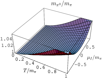
Figure 3.2: $m_{\pi^{0}}$ as a function of $T$ and $\mu_{\mbox{\tiny I}}$ in units of $m_{\pi}$.

Figure 3.2 shows the dependence of the $\pi^{0}$ mass as a function of temperature and isospin chemical potential. It is a growing function of both variables, temperature and $|\mu_{\mbox{\tiny I}}|$.

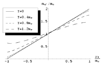
Figure 3.3: $m_{\pi^{-}}$ as a function of $\mu_{\mbox{\tiny I}}$ for fixed values of $T$ in units of $m_{\pi}$.

From Figure 3.3 we see that, at zero temperature, we agree with the usual prediction, $m_{\pi^{-}}=m_{\pi}+\mu_{\mbox{\tiny I}}$. In fact, at zero temperature, the $\pi^{-}$ should condense when $\mu_{\mbox{\tiny I}}=-m_{\pi}$ (the inverse situation occurs for $\pi^{+}$). Now, this situation changes if temperature starts to grow. The condensation point no longer occurs at $\mu_{\mbox{\tiny I}}=-m_{\pi}$, but it moves to the left, i.e. to a bigger (in absolute value) chemical potential. In the vicinity of $\mu_{\mbox{\tiny I}}=m_{\pi}$ the mass starts to decrease. This figure shows the $\pi^{-}$ mass in the normal phase only, $|\mu_{\mbox{\tiny I}}|<m_{\pi}$. Even though we can consider higher values for the isospin chemical potential in the first phase, since $m>m_{\pi}$ (see appendix B.2), this situation will be discussed in the next chapter.

For the case of the $\pi^{+}$ mass, the behavior is the same, exchanging $\mu_{\mbox{\tiny I}}$ for $-\mu_{\mbox{\tiny I}}$.

3.2 Decay constant

In connection with the behavior of $f_{\pi}(T,\mu_{\mbox{\tiny I}})$ when $\mu_{\mbox{\tiny I}}<m_{\pi}$, we have made use of PCAC, which provides us with a relation between the renormalized propagator and the pion decay constant.

The axial current is obtained as the functional derivative of the action with respect to $a_{\mu}^{a}$, with $a_{\mu}=a_{\mu}^{a}\tau^{a}/2$

$$A_{\mu}^{a}=\frac{\delta S_{\chi}}{\delta a_{\mu}^{a}}(M,0,\mu_{\mbox{\tiny I}}u{\textstyle\frac{1}{2}}\tau_{3},0)$$ (3.19)

The expansion of the axial current in terms of powers of the pion fields can be found in detail in Appendix A.2.1. Defining $A^{\pm}_{\mu}\equiv\frac{1}{\sqrt{2}}\big{(}A^{1}_{\mu}\mp iA^{2}_{\mu}\big{)}$, the axial current is

$$A_{(1,1)}^{0} = -f\partial\pi^{0}$$ (3.20)

$$A_{(1,1)}^{\pm} = -f(\partial_{I}\pi)^{\pm}$$

$$A_{(1,3)}^{0} = \frac{2}{3f}\big{[}2|\pi|^{2}\partial\pi^{0}-\pi^{0}\partial|\pi|^{2}\big{]}$$ (3.21)

$$A_{(1,3)}^{\pm} = \frac{1}{3f}\big{[}2(\pi_{0}^{2}+2|\pi|^{2})(\partial_{I}\pi)_{\pm}-\pi_{\pm}\partial(\pi_{0}^{2}+2|\pi|^{2})\big{]}$$ (3.22)

$$A_{(3,1)}^{0} = -\frac{1}{f}2m^{2}l_{4}\partial\pi^{0}$$ (3.23)

$$A_{(3,1)}^{\pm} = -\frac{1}{f}2m^{2}l_{4}(\partial_{I}\pi)^{\pm}$$ (3.24)

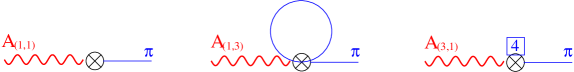
Figure 3.4: Diagramatic contribution to the PCAC relation at one-loop corrections.

Saturating the axial current with a single pion (the reduction formula can be found in Appendix B.7), we obtain

$$\langle\!\langle 0|A_{\mu}^{0}|\pi_{R}^{0}(p)\rangle\!\rangle = ip_{\mu}f\Big{\{}\sqrt{Z_{0}}+\alpha\big{[}-{\textstyle\frac{2}{3}}\underline{\lambda}+2\bar{l}_{4}-{\textstyle\frac{16}{3}}I\big{]}\Big{\}},$$ (3.25)

$$\langle\!\langle 0|A^{\pm}|\pi_{R}^{\mp}(p)\rangle\!\rangle = i(p\pm\mu_{\mbox{\tiny I}}u)f\Big{\{}\sqrt{Z_{\pm}}+\alpha\big{[}-{\textstyle\frac{2}{3}}\underline{\lambda}+2\bar{l}_{4}-{\textstyle\frac{8}{3}}(I_{0}+I)\big{]}\Big{\}}$$ (3.26)

$$\mp iu_{\mu}f\epsilon(\mu_{\mbox{\tiny I}})\alpha 8mJ.$$

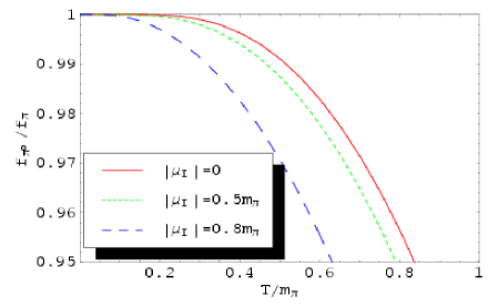
a. b.

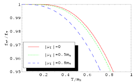
Figure 3.5: a. Neutral pion decay constant and b. charged pions decay constant at finite temperature and isospin chemical potential

The different contributions to the PCAC relation in the expansion of the axial current are shown in Figure 3.4. Using the values of the renormalization constants $Z_{a}$ in equations (3.8) and (3.9), the renormalized PCAC relation is

$$\langle\!\langle 0|A^{0}|\pi_{R}^{0}(p)\rangle\!\rangle = ipf\Big{\{}1+\alpha\big{[}\bar{l}_{4}-4I\big{]}\Big{\}},$$ (3.27)

$$\langle\!\langle 0|A^{\pm}|\pi_{R}^{\mp}(p)\rangle\!\rangle = i(p\pm\mu_{\mbox{\tiny I}}u)\Big{\{}1+\alpha\big{[}\bar{l}_{4}-2(I+I_{0})\big{]}\Big{\}}\mp iu\epsilon(\mu_{\mbox{\tiny I}})8\alpha fmJ.$$ (3.28)

Then, we define the effective decay constant as the part proportional to $p_{\mu}$, so

$$f_{\pi^{0}}(T,\mu_{I}) \equiv f\Big{\{}1+\alpha\big{[}\bar{l}_{4}-4I\big{]}\Big{\}},$$

$$f_{\pi^{\pm}}(T,\mu_{I}) \equiv f\Big{\{}1+\alpha\big{[}\bar{l}_{4}-2(I+I_{0})\big{]}\Big{\}}.$$ (3.29)

We can see that, at zero temperature and chemical potential, we obtain the usual pion decay constant

$$f_{\pi}=f\big{[}1+\alpha\bar{l}_{4}\big{]}\approx 92.5\mbox{MeV}.$$ (3.30)

For an increasing chemical potential, the couplings $f_{\pi}(T,\mu_{\mbox{\tiny I}})$ decrease faster (Fig. 3.5). This effect is enhanced for $f_{\pi_{0}}(T,\mu_{\mbox{\tiny I}})$ (Fig. 3.5.a) and is related to the fact that $f_{\pi^{0}}(T,\mu_{\mbox{\tiny I}})$ only receives radiative corrections from charged pion loops; in contrast, $f_{\pi^{\pm}}(T,\mu_{\mbox{\tiny I}})$ receives both loop contributions, from charged pions and for neutral pions. For the case of zero chemical potential, $f_{\pi}(T)$ is again the same one for the three pions,

$$f_{\pi}(T)=f\left[1+\alpha\left(\bar{l}_{4}-4I_{0}\right)\right].$$ (3.31)

3.3 Condensates.

There are three kinds of condensates relevant for the present analysis: the chiral condensate $\langle\!\langle\bar{q}q\rangle\!\rangle$, responsible for the spontaneous chiral symmetry breaking; the pion condensate $\langle\!\langle\bm{\pi}\rangle\!\rangle$, which gives us information about the pions in the condensed phase; and the isospin number density $\langle\!\langle n_{I}\rangle\!\rangle$, which tells us about the difference of $u$ and $d$ baryon number inside the thermal bath. The expansions of the currents are explained in detail in Appendix A.2. In the case of the first phase, as is expected, the pion condensate is equal to zero.

3.3.1 Chiral condensate.

The chiral condensate can be defined as the expectation value of the scalar current in the vacuum, $\langle\!\langle\bar{q}q\rangle\!\rangle=\langle\!\langle 0|J_{s}|0\rangle\!\rangle$, with the scalar current for massive quarks at finite isospin chemical potential defined as

$$J_{s}=\frac{\delta S_{\chi}}{\delta s^{0}}(M,0,{\textstyle\frac{1}{2}}\mu_{\mbox{\tiny I}}u\tau_{3},0)$$ (3.32)

The components needed for radiative corrections are

$$\langle\!\langle J_{s(1,0)}\rangle\!\rangle = -2Bf^{2}$$ (3.33)

$$\langle\!\langle J_{s(1,2)}\rangle\!\rangle = B\langle\!\langle 0|\pi_{0}^{2}+2|\pi|^{2}|0\rangle\!\rangle$$ (3.34)

$$\langle\!\langle J_{s(3,0)}\rangle\!\rangle = -4Bm^{2}(l_{3}+l_{4}+\tilde{h}_{1}).$$ (3.35)

Using the fact that

$$\langle\!\langle 0|\pi_{a}(x)\pi_{b}(x)|0\rangle\!\rangle=\langle\!\langle 0|T\pi_{a}(x)\pi_{b}(y)|0\rangle\!\rangle_{y=x},$$ (3.36)

the corrected chiral condensate turns out to be

$$\langle\!\langle\bar{q}q\rangle\!\rangle(T,\mu_{\mbox{\tiny I}})=-2Bf^{2}\left\{1-\alpha\left[{\textstyle\frac{1}{2}}\bar{l}_{3}-2\bar{l}_{4}-32\pi^{2}\tilde{h}_{1}+2I_{0}+4I\right]\right\},$$ (3.37)

where the chiral condensate at zero temperature and chemical potential is

$$\langle\bar{q}q\rangle=-2Bf^{2}\big{[}1-\alpha\big{(}{\textstyle\frac{1}{2}}\bar{l}_{3}-2\bar{l}_{4}-32\pi^{2}\tilde{h}_{1}\big{)}\big{]},$$ (3.38)

and the chiral condensate at finite temperature and zero chemical potential is

$$\langle\!\langle\bar{q}q\rangle\!\rangle(T)=-2Bf^{2}\left\{1-\alpha\left[{\textstyle\frac{1}{2}}\bar{l}_{3}-2\bar{l}_{4}-32\pi^{2}\tilde{h}_{1}+6I_{0}\right]\right\}.$$ (3.39)

The constant $\tilde{h}_{1}$, as was said before, is model dependent. If we accept the G-MOR relation

$$m_{\pi}^{2}f_{\pi}^{2}=-\frac{1}{2}(m_{u}+m_{d})\langle\bar{q}q\rangle,$$ (3.40)

neglecting the term $\epsilon_{ud}^{2}l_{7}$ that appears in the $m_{\pi^{0}}$ corrections, we find from equations (3.17) and (3.30) that

$$m_{\pi}^{2}f_{\pi}^{2}=(m_{u}+m_{d})Bf^{2}\big{[}1-\alpha({\textstyle\frac{1}{2}}\bar{l}_{3}-2\bar{l}_{4})\big{]}.$$ (3.41)

Comparing with eq. (3.38), if we consider the G-MOR relation as valid, we can set $\tilde{h}_{1}=0$.

Figure 3.6 shows the chiral condensate at finite temperature and isospin chemical potential. It has a similar behavior as the pion decay constants in Figure 3.5.

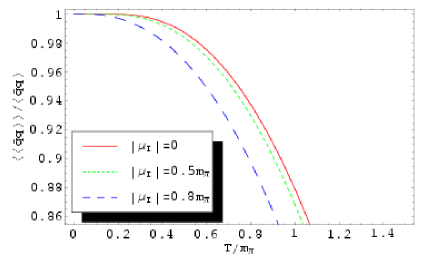
Figure 3.6: Quark condensate as a function of the temperature and the isospin chemical potential

G-MOR relation at finite temperature and isospin chemical potential

If we set $\tilde{h}_{1}=0$, $\epsilon_{ud}^{2}l_{7}\sim 0$, from equations (3.18) and (3.31) we obtain

$$m_{\pi}(T)^{2}f_{\pi}(T)^{2}=\left[1-\alpha\left({\textstyle\frac{1}{2}}\bar{l}_{3}-2\bar{l}_{4}+6I_{0}\right)\right].$$ (3.42)

Compared with equation (3.39) we can see that the G-MOR relation is still valid.

At finite chemical potential, however, this relation in not possible, since the states are not degenerate. This suggests to extend this relation using the average value of the results.

First of all, we have to take into account that the tree-level part of this average cannot depend on the chemical potential. Observing equations (3.15) and (3.16), we can see that the only possibility is to use the average of the pion masses and the pion decay constants. Defining

$$\overline{m}_{\pi}(T,\mu_{\mbox{\tiny I}}) \equiv {\textstyle\frac{1}{3}}\left[m_{\pi^{+}}(T,\mu_{\mbox{\tiny I}})+m_{\pi^{-}}(T,\mu_{\mbox{\tiny I}})+m_{\pi^{0}}(T,\mu_{\mbox{\tiny I}})\right]$$ (3.43)

$$= m\left\{1+\alpha\left[-{\textstyle\frac{1}{4}}\bar{l}_{3}-{\textstyle\frac{1}{3}}32\pi^{2}\epsilon_{ud}^{2}l_{7}+{\textstyle\frac{1}{3}}(I_{0}+2I)\right]\right\},$$

$$\overline{f}_{\pi}(T,\mu_{\mbox{\tiny I}}) \equiv {\textstyle\frac{1}{3}}\left[f_{\pi^{+}}(T,\mu_{\mbox{\tiny I}})+f_{\pi^{-}}(T,\mu_{\mbox{\tiny I}})+f_{\pi^{0}}(T,\mu_{\mbox{\tiny I}})\right]$$ (3.44)

$$= f\left\{1+\alpha\left[\bar{l}_{4}-{\textstyle\frac{4}{3}}(I_{0}+2I)\right]\right\},$$

and combining the quadratic terms, we find

$$\overline{m}_{\pi}(T,\mu_{\mbox{\tiny I}})^{2}\overline{f}_{\pi}(T,\mu_{\mbox{\tiny I}})^{2}=(m_{u}+m_{d})Bf^{2}\left\{1+\alpha\left[-{\textstyle\frac{1}{2}}\bar{l}_{3}+2\bar{l}_{4}-{\textstyle\frac{1}{3}}32\pi^{2}\epsilon_{ud}^{2}l_{7}-2I_{0}-4I\right]\right\}.$$ (3.45)

This result is exactly $-{\textstyle\frac{1}{2}}(m_{u}+m_{d})\langle\!\langle\bar{q}q\rangle\!\rangle$ in equation (3.37) but with $\tilde{h}_{1}={\textstyle\frac{1}{3}}\epsilon_{ud}^{2}l_{7}$. We can say that the generalized G-MOR relation is

$$\overline{m}_{\pi}^{2}\overline{f}_{\pi}^{2}=-{\textstyle\frac{1}{2}}(m_{u}+m_{d})\langle\!\langle\bar{q}q\rangle\!\rangle.$$ (3.46)

3.3.2 Isospin-number density.

The isospin-number density condensate gives us information about the baryon number difference between $u$ and $d$ quarks in the thermal vacuum or populated vacuum. The isospin-number density is defined as the 0-Lorentz and 3-isospin component of the vector current

$$n_{I}\equiv{\textstyle\frac{1}{2}}q^{\dagger}\tau^{3}q=V_{0}^{3}.$$ (3.47)

We need to calculate the expectation value of the vector current in the vacuum. We will see that the only non-vanishing component of the vector current in the vacuum is the isospin-number density.

Considering the expansion of the vector current explained in appendix A.2.3 and using the fact that

$$\langle\!\langle 0|\pi_{a}|0\rangle\!\rangle=0,\qquad\langle\!\langle 0|\pi_{a\neq 3}\pi_{3}|0\rangle\!\rangle=0,$$ (3.48)

we find that the only non-zero component of the vector current in the vacuum, for the first phase case, is

$$\langle\!\langle\bm{V}_{(1,2)\mu}\rangle\!\rangle=\langle\!\langle 0|-i(\pi_{\mbox{\tiny$+$}}\partial_{\mu}\pi_{\mbox{\tiny$-$}}-\pi_{\mbox{\tiny$-$}}\partial_{\mu}\pi_{\mbox{\tiny$+$}})+2\mu_{\mbox{\tiny I}}|\pi|^{2}u_{\mu}|0\rangle\!\rangle\bm{e}_{3}.$$ (3.49)

Using the fact that

$$\langle\!\langle 0|\pi^{a}(x)\partial\pi^{b}(x)|0\rangle\!\rangle=\Big{[}\partial_{y}\langle\!\langle 0|T\pi^{a}(x)\pi^{b}(y)|0\rangle\!\rangle\Big{]}_{y=x},$$ (3.50)

$$\langle\!\langle\bm{V}_{\mu}\rangle\!\rangle=8mf^{2}\alpha\epsilon(\mu_{\mbox{\tiny I}})Ju_{\mu}\bm{e}_{3}~{}=~{}\langle\!\langle n_{I}\rangle\!\rangle u_{\mu}\bm{e}_{3}.$$ (3.51)

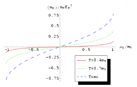
Figure 3.7: Isospin-number density condensate as a function of the isospin chemical potential for different values of the temperature.

Figure 3.7 shows the isospin-number density expectation value in the thermal vacuum. It gets a non vanishing value only inside the thermal bath.

If we compare the results of the PCAC relation for charged pions in equation (3.26), we find that the term proportional to $u_{\mu}$ is exactly the isospin-number density condensate

$$\langle\!\langle 0|A_{\mu}^{\pm}|\pi^{\mp}\rangle\!\rangle=i(p_{\mu}\pm\mu_{\mbox{\tiny I}}u_{\mu})f_{\pi^{\pm}}(T,\mu_{\mbox{\tiny I}})\mp iu_{\mu}\langle\!\langle n_{I}\rangle\!\rangle.$$ (3.52)

Chapter 4 Thermal pions in the second phase for $|\mu_{\mbox{\tiny I}}|\gtrsim m$

In chapter 2, I presented a systematic expansion method for radiative calculations in the second phase. For the case of the chemical potential near the transition point between the two phases, it is possible to expand the radiative corrections in powers of $s^{2}$:

$$\Sigma(p;f,m;T,\mu_{\mbox{\tiny I}})=\alpha^{\prime}\sum_{n=0}\sigma_{n}(\bar{p},\bar{T})s^{2n}.$$ (4.1)

If we consider the lowest order in this expansion, ${\cal O}(s^{0})$, we find that the vertices and propagators are the same as in the case of the first phase. The only difference is that the factors $m$ are changed by $|\mu_{\mbox{\tiny I}}|$. I remark that in this phase a negative chemical potential $\mu_{\mbox{\tiny I}}=-|\mu_{\mbox{\tiny I}}|$, will be considered where the negative pion will condense.

4.1 Masses

Proceeding with the relevant vertices and propagators, the loop corrections to the pion propagator matrix are shown in Figures 2.1 and 2.2, respectively.

Defining $\underline{\lambda}^{\prime}=\lambda-\ln(\mu_{\mbox{\tiny I}}^{2}/\Lambda^{2})$, the self-energy is

$$\Sigma(p)_{{\mbox{\tiny$00$}}} = \alpha^{\prime}\Big{\{}-\mu_{\mbox{\tiny$I$}}^{2}\big{[}{\textstyle\frac{4}{3}}\underline{\lambda}+{\textstyle\frac{1}{2}}\bar{l}_{3}-2\bar{l}_{4}+32\pi^{2}\epsilon-{ud}^{2}l_{7}+2I^{\prime}_{0}-{\textstyle\frac{4}{3}}I^{\prime}\big{]}$$ (4.2)

$$\hskip 170.71652pt+p^{2}\big{[}{\textstyle\frac{4}{3}}\underline{\lambda}-2\bar{l}_{4}+{\textstyle\frac{8}{3}}I^{\prime}\big{]}\Big{\}},$$

$$\Sigma(p)_{{\mbox{\tiny$-+$}}} = \alpha^{\prime}\Big{\{}-\mu_{\mbox{\tiny$I$}}^{2}\big{[}{\textstyle\frac{1}{2}}\bar{l}_{3}+32\pi^{2}\epsilon_{ud}^{2}l_{7}-2I^{\prime}_{0}-8J^{\prime}\big{]}+p^{2}\big{[}{\textstyle\frac{4}{3}}\underline{\lambda}-2\bar{l}_{4}+{\textstyle\frac{4}{3}}I^{\prime}_{0}+{\textstyle\frac{4}{3}}I^{\prime}\big{]}$$ (4.3)

$$\hskip 128.0374pt-2p_{0}|\mu_{\mbox{\tiny$I$}}|\big{[}{\textstyle\frac{4}{3}}\underline{\lambda}-2\bar{l}_{4}+{\textstyle\frac{4}{3}}I^{\prime}_{0}+{\textstyle\frac{4}{3}}I^{\prime}+4J^{\prime}\big{]}\Big{\}},$$

$$\Sigma(p)_{{\mbox{\tiny$+-$}}} = \Sigma(-p)_{{\mbox{\tiny$-+$}}}.$$ (4.4)

These self-energies include also higher correction terms of ${\cal O}(s^{2})$. Now $\alpha^{\prime}=(\mu_{\mbox{\tiny I}}/4\pi f)^{2}$ is the perturbative term, and the functions $I^{\prime}$, $J^{\prime}$, $I^{\prime}_{n}$ are defined as follows:

$$I^{\prime} \equiv \int_{1}^{\infty}dx\sqrt{x^{2}-1}\Big{[}n_{B}\big{(}|\mu_{\mbox{\tiny I}}|(x-1)\big{)}+n_{B}\big{(}|\mu_{\mbox{\tiny I}}|(x+1)\big{)}\Big{]},$$ (4.5)

$$J^{\prime} \equiv \int_{1}^{\infty}dxx\sqrt{x^{2}-1}\Big{[}n_{B}\big{(}|\mu_{\mbox{\tiny I}}|(x-1)\big{)}-n_{B}\big{(}|\mu_{\mbox{\tiny I}}|(x+1)\big{)}\Big{]},$$ (4.6)

$$I^{\prime}_{n} \equiv \int_{1}^{\infty}dx\sqrt{x^{2}-1}x^{2n}2n_{B}\big{(}|\mu_{\mbox{\tiny$I$}}|x\big{)}.$$ (4.7)

Note that these definitions are almost the same ones we used in the first phase. Here, however, the term that multiplies $x$ in the argument of the Bose-Einstein distribution is $\mu_{\mbox{\tiny I}}$ instead of $m$.

Following the prescription, indicated in section 1.1.3, that the renormalized self-energy does not depend on $p^{2}$, we have that the renormalization constants are

$$Z_{0} = 1+\alpha^{\prime}\big{[}{\textstyle\frac{4}{3}}\underline{\lambda}-2\bar{l}_{4}+{\textstyle\frac{8}{3}}I^{\prime}\big{]},$$

$$Z_{\pm} = 1+\alpha^{\prime}\big{[}{\textstyle\frac{4}{3}}\underline{\lambda}-2\bar{l}_{4}+\frac{4}{3}I^{\prime}_{0}+{\textstyle\frac{4}{3}}I^{\prime}\big{]},$$ (4.8)

and the renormalized self-energy corrections are then

$$\Sigma_{R{\mbox{\tiny$00$}}} = \mu_{\mbox{\tiny I}}^{2}\alpha^{\prime}\big{[}-{\textstyle\frac{1}{2}}\bar{l}_{3}-32\pi^{2}\epsilon_{ud}^{2}l_{7}-2I^{\prime}_{0}+4I^{\prime}\big{]},$$

$$\Sigma_{R}(p_{0})_{\mbox{\tiny$-+$}} = \alpha^{\prime}\Big{\{}\mu_{\mbox{\tiny$I$}}^{2}\big{[}-{\textstyle\frac{1}{2}}\bar{l}_{3}+2I^{\prime}_{0}+8J^{\prime}\big{]}-8|\mu_{\mbox{\tiny$I$}}|J^{\prime}p_{0}\Big{\}},$$

$$\Sigma_{R}(p_{0})_{\mbox{\tiny$+-$}} = \Sigma_{R}(-p_{0})_{\mbox{\tiny$-+$}},$$ (4.9)

plus higher corrections of order $\mu_{\mbox{\tiny I}}^{2}\alpha^{\prime}s^{2}$. We will use these results to extract the renormalized temperature- and chemical potential-dependent masses.

To extract the $m_{\pi^{\mbox{\tiny$0$}}}$ mass, we do not need any further effort, since it is already diagonal in the matrix propagator, and its renormalized self-energy is constant in the external momenta, i.e., it does not depend on $p_{0}$:

$$m_{\pi^{\mbox{\tiny$0$}}}=|\mu_{\mbox{\tiny I}}|\Big{\{}1+\alpha^{\prime}\big{[}-{\textstyle\frac{1}{4}}\bar{l}_{3}-16\pi^{2}\epsilon_{ud}^{2}l_{7}-I^{\prime}_{0}+2I^{\prime}\big{]}\Big{\}}.$$ (4.10)

For the case of $m_{\pi^{\mbox{\tiny$\pm$}}}$, the vanishing determinant of the charged matrix propagator, provides us with a second-order equation in powers of $p_{0}^{2}$:

$$p_{0}^{4}-p_{0}^{2}\Big{[}m_{+}^{2}+2\Sigma_{R{\mbox{\tiny$-+$}}}^{\mbox{\tiny$0$}}+4|\mu_{\mbox{\tiny I}}|c\Sigma_{R{\mbox{\tiny$-+$}}}^{\mbox{\tiny$1$}}+(\Sigma_{R{\mbox{\tiny$-+$}}}^{\mbox{\tiny$1$}})^{2}\Big{]}+s^{2}\mu_{\mbox{\tiny I}}^{2}\Sigma_{R{\mbox{\tiny$-+$}}}^{\mbox{\tiny$0$}}+(\Sigma_{R{\mbox{\tiny$-+$}}}^{\mbox{\tiny$0$}})^{2}=0.$$ (4.11)

The solution of this equation gives the $\pi^{\pm}$ masses, recognizing them respectively according to the tree-level case. We can write the expression for the masses in a more compact way, by expanding around the $m_{+}$ term that appears in the last equation. The $\pi^{+}$ mass is given by

$$m_{\pi^{+}}=m_{+}+\alpha^{\prime}|\mu_{\mbox{\tiny I}}|\big{[}-{\textstyle\frac{1}{4}}\bar{l}_{3}+I^{\prime}_{0}-4J^{\prime}+{\cal O}(s^{2})\big{]}.$$ (4.12)

Some care has to be taken in the extraction of the $\pi^{-}$ mass. For the case of $m_{\pi^{0}}$ and $m_{\pi^{+}}$, since they have a tree-level mass, it is possible to consider them as

$$m_{R}(T,\mu_{\mbox{\tiny I}})=m_{t}(\mu_{\mbox{\tiny I}})\left[1+\alpha^{\prime}\sigma(T,s)\right],$$ (4.13)

and, then, we can expand the corrections in terms of $s$ (or $c$ in the other limit). For the case of the $\pi^{-}$ mass, if we consider the expansion in mass corrections explained in chapter 1.1.3, calculating the determinant of the propagator matrix, at the lowest order, we obtain a second-order equation for the $\delta m_{-}$ mass correction (which is the $\pi^{-}$ mass since it does not have a tree-level mass). The result will be of the form

$$|\mu_{\mbox{\tiny I}}|\delta m_{-}=s^{2}\Sigma_{A}+\sqrt{s^{2}\mu_{\mbox{\tiny I}}^{2}\Sigma_{B}+(s^{2}\Sigma_{A})^{2}+\Sigma_{C}\Sigma_{D}+\Sigma_{E}^{2}}.$$ (4.14)

This mixes terms of order $\alpha^{\prime}$ and $\sqrt{{\cal O}(\alpha^{\prime})+{\cal O}(\alpha^{\prime 2})}$, so all these self-energy terms must be expanded independently in powers of $s$ (or $c$). With this criterion in mind, the $\pi^{-}$ mass is then

$$m_{\pi^{-}}(T,\mu_{\mbox{\tiny I}})=\theta(T_{c}){\textstyle\frac{1}{2}}\sqrt{s^{2}\mu_{\mbox{\tiny I}}^{2}\Sigma_{R{\mbox{\tiny$-+$}}}^{\mbox{\tiny$0$}}+(\Sigma_{R{\mbox{\tiny$-+$}}}^{\mbox{\tiny$0$}})^{2}},$$ (4.15)

with

$$\Sigma_{R{\mbox{\tiny$-+$}}}^{\mbox{\tiny$0$}}=\alpha^{\prime}[-{\textstyle\frac{1}{2}}\bar{l}_{3}+2I^{\prime}_{0}+8J^{\prime}],$$ (4.16)

and $T_{c}$ is the critical temperature, where the $\pi^{-}$ mass is zero at the transition point from the first to the second phase, i.e., when $\mu_{\mbox{\tiny I}}=m$:

$$m_{\pi^{-}}(T_{c},m)=0,\qquad T_{c}\approx 0.135m_{\pi}=18.9\mbox{MeV}$$ (4.17)

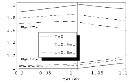
Figure 4.1: $m_{\pi^{0}}$ and $m_{\pi^{+}}$ as a function of high values of the isospin chemical potential at different values of temperature. All parameters are scaled with $m_{\pi}$

To start the discussion, I would like to mention that, near the transition point, $m_{\pi^{+}}$ decreases, as in the tree-level approximation, and this behavior is enforced with temperature. In this region, $m_{\pi^{0}}$ grows with both parameters (see Figure 4.1).

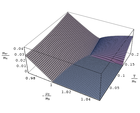
Figure 4.2: $m_{\pi^{-}}(T,\mu_{\mbox{\tiny I}})$. All the parameters are scaled with $m_{\pi}$

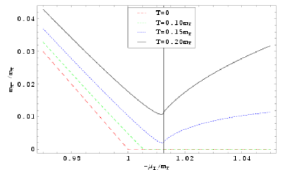
Figure 4.3: $m_{\pi^{-}}$ plot versus isospin chemical potential for different temperatures. All values are scaled with $m_{\pi}$. The vertical line corresponds to $\mu_{\mbox{\tiny I}}=m$.

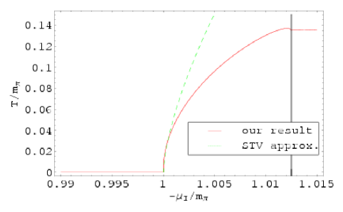
Figure 4.4: Phase diagram of the condensation point of temperature versus isospin chemical potential. The dashed line corresponds to the approximation made by Splittorff, Toublan and Veerbarschot [STV02b].

For $m_{\pi^{-}}$, according to Figures 4.2 and 4.3, we see that a certain critical temperature must be reached before the $\pi^{-}$ is removed from the condensed state. This is precisely the condition that determines the phase transition curve (Fig. 4.4).

Starting from the first phase, according to the previous chapter, for $T<m_{\pi}$, it is possible to find, at first order in $T$, an expression for the transition line $\mu_{\mbox{\tiny I}}(T)$ that coincides with the results given in eq. (8.91) from [STV02b]. In Fig. 4.4, the dashed line corresponds to this approximation, valid at low temperature. However, this result gives us the transition line from the viewpoint of the first phase.

The reader could think from Fig. 4.4 that the critical temperature remains constant in the second phase. However, the temperature actually rises as a function of the chemical potential, in the form

$$T_{trans}(\mu_{\mbox{\tiny I}})=\frac{T_{c}}{m}|\mu_{\mbox{\tiny I}}|\approx 0.134|\mu_{\mbox{\tiny I}}|.$$ (4.18)

The slope is very smooth, and therefore we cannot appreciate this behavior from the values shown in the figure. This growing behavior of the critical temperature is of course consistent with general statements about phase transitions in the Ginzburg-Landau theory and it has been actually calculated in the lattice for two or three color QCD. Nevertheless, if we consider the thermal corrections in the second phase, it happens that the condensation phenomenon starts to disappear for a certain value of $T>18.9$MeV near the transition point, leaving a kind of superfluid state which includes the condensed as well as the normal phase (massive pion modes).

4.2 Condensates.

As was said at the beginning of this chapter, the different propagators and vertices are almost the same as in the first phase if we consider the zeroth order in the radiative corrections (just changing $m$ by $|\mu_{\mbox{\tiny I}}|$ and $\mu_{\mbox{\tiny I}}$ by $-\mu_{\mbox{\tiny I}}$). In this case, the same occurs, as in the expansion of the different currents.

4.2.1 Chiral condensate.

Following the same procedure in the case of the first phase, the non-vanishing components of the chiral condensate at order $s^{0}$ are

$$\langle\!\langle J_{s(1,0)}\rangle\!\rangle = -2Bf^{2}c,$$ (4.19)

$$\langle\!\langle J_{s(1,3)}\rangle\!\rangle = Bc\langle\!\langle 0|\pi_{0}^{2}+2|\tilde{\pi}|^{2}|0\rangle\!\rangle,$$ (4.20)

$$\langle\!\langle J_{s(1,0)}\rangle\!\rangle = -4B\mu_{\mbox{\tiny I}}^{2}c(l_{3}+l_{4}+\tilde{h}_{1}).$$ (4.21)

The term $c$ must be kept because it is a global constant.

The resulting chiral condensate at finite temperature and isospin chemical potential is then

$$\langle\!\langle\bar{q}q\rangle\!\rangle=-2Bf^{2}c\{1+\alpha^{\prime}[-{\textstyle\frac{1}{2}}\bar{l}_{3}+2\bar{l}_{4}-2I^{\prime}_{0}-4I^{\prime}\}.$$ (4.22)

In Figure 4.5, we can see the transition of the chiral condensate from the first phase to the second phase. Now, the chiral condensate in the second phase tends to decrease abruptly with the chemical potential. This effect is enhanced by temperature..

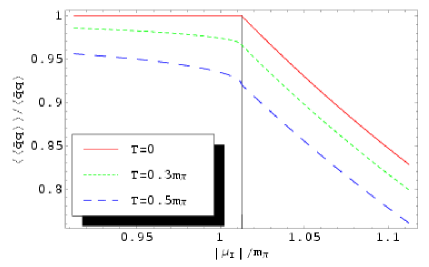
Figure 4.5: Chiral condensate as a function of the isospin chemical potential for different values of the temperature. The vertical line denotes the transition point between the two phases.

4.2.2 Isospin-number density.

The non-vanishing components of the condensed vector current at order $s^{0}$ are

$$\langle\!\langle\bm{V}\rangle\!\rangle_{(1,0)} = -f^{2}|\mu_{\mbox{\tiny I}}|s^{2}{\bf e}_{3}u,$$ (4.23)

$$\langle\!\langle\bm{V}\rangle\!\rangle_{(1,2)} = \langle\!\langle 0|-i(\tilde{\pi}_{1}\partial\tilde{\pi}_{2}-\tilde{\pi}_{2}\partial\tilde{\pi}_{1})-2|\mu_{\mbox{\tiny I}}||\tilde{\pi}|^{2}u|0\rangle\!\rangle{\bf e}_{3}.$$ (4.24)

Like in the case fot the calculation of $m_{\pi^{-}}$, we have to keep the tree-level part proportional to $s^{2}$.

The isospin-number density condensate at finite temperature and chemical potential is then

$$\langle\!\langle n_{I}\rangle\!\rangle=-|\mu_{\mbox{\tiny I}}|f^{2}[s^{2}+8\alpha^{\prime}J^{\prime}].$$ (4.25)

In Figure 4.6, we can see the transition of the isospin number density from the first phase to the second phase. Like the chiral condensate, in the second phase $\langle\!\langle n_{I}\rangle\!\rangle$ tends to decrease abruptly with the chemical potential. Once again this effect is enhanced by temperature.

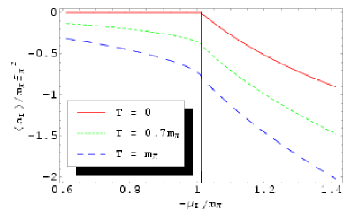
Figure 4.6: Isospin number density as a function of the isospin chemical potential for different values of the temperature.

4.2.3 Pion condensate.

Now, in the second phase, the pion condensate is finite and give us important information about the condensed phase. The pion condensate is defined as

$$\langle\!\langle\pi^{a}\rangle\!\rangle\equiv\langle\!\langle 0|\bar{q}i\gamma_{5}\tau^{a}q|0\rangle\!\rangle=\langle\!\langle 0|J_{p}^{a}|0\rangle\!\rangle,$$ (4.26)

and is, like the other condensates, a QCD vacuum-state operator with the same quantum numbers of the pion field. From Appendix A.2.4, the non-vanishing components of the pion condensates are

$$\langle\!\langle\bm{J}_{p(1,0)}\rangle\!\rangle = -2Bf^{2}s\tilde{\bf e}_{1}$$ (4.27)

$$\langle\!\langle\bm{J}_{p(1,3)}\rangle\!\rangle = Bc\langle\!\langle 0|\pi_{0}^{2}+2|\pi|^{2}|0\rangle\!\rangle\tilde{\bf e}_{1}$$ (4.28)

$$\langle\!\langle\bm{J}_{p(1,0)}\rangle\!\rangle = -4B\mu_{\mbox{\tiny I}}^{2}c(l_{3}+l_{4})\tilde{\bf e}_{1}.$$ (4.29)

As we did for the chiral condensate, we must keep the term $s$, since it is a global factor. We can see that the pion condensate is oriented in the direction ${\bf e}_{1}$, i.e., $\langle\!\langle\bm{\pi}\rangle\!\rangle=\langle\!\langle\tilde{\pi}_{1}\rangle\!\rangle\tilde{\bf e}_{1}$.

Proceeding in the same way as we did with the other condensates, the pion condensate at finite temperature and isospin chemical potential is

$$\langle\!\langle\tilde{\pi}_{1}\rangle\!\rangle=2Bf^{2}s\{1+\alpha^{\prime}[-{\textstyle\frac{1}{2}}\bar{l}_{3}+2\bar{l}_{4}-2I^{\prime}_{0}-4I^{\prime}]\}.$$ (4.30)

It is important to recall that the pion condensates, like the chiral condensate, give an information about the quarks condensed in the vacuum; in this case the pion condensate is a mixture of $\bar{u}\gamma_{5}d$ and $\bar{d}\gamma_{5}u$. This condensate breaks parity.

Note that this result is basically the same as the chiral condensate (except the global factors $s$ and $-c$) if we neglect the term $\tilde{h}_{1}$. Then the chiral condensate and pion condensate satisfy the relation

$$s\langle\!\langle\bar{q}q\rangle\!\rangle+c\langle\!\langle\tilde{\pi}_{1}\rangle\!\rangle=0.$$ (4.31)

We will see that this relation is valid in the limit when $|\mu_{\mbox{\tiny I}}|\gg m$.

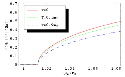
Figure 4.7: Pion condensate as a function of the isospin chemical potential for different values of the temperature. The vertical line denotes the transition point between the two phases.

Figure 4.7 shows the behavior of the pion condensate at finite temperature and isospin chemical potential. If we compare with Figure 4.5, we can see that the chiral condensate diminishes with the chemical potential in a similar rate as the pion condensate. This means that the quarks in the chiral condensate mix together to form mixed $u$-$d$ pseudo-scalar Cooper-pairs state. Due to the thermal bath, both chiral and pion condensates decrease, as expected, due to the increase of the $\pi^{-}$ mass due to the thermal bath.

Chapter 5 Thermal pions in the second phase for $|\mu_{\mbox{\tiny I}}|\gg m$

In this chapter, we will finish the analysis of the in-medium radiative correction to the masses and condensates in the region of high isospin chemical potential. As in the previous section, we will expand the different corrections to the propagators and the condensates, but this time in powers of $c$. Nevertheless, we have to include a logarithmic term in the expansion since loop corrections give rise to terms of the form $\lambda-\ln(\mu_{\mbox{\tiny I}}^{2}/\Lambda^{2})$, which cancel with the terms $\lambda-\ln(m^{2}/\Lambda^{2})$ coming from the $l_{i}$ coupling constants. The radiative corrections can be expanded as

$$\Sigma(p;T,\mu_{\mbox{\tiny I}};m,f)=\alpha^{\prime}\sum_{n=0}\left[\sigma_{n}(\bar{p},\bar{T})+\sigma_{n}^{\mbox{\tiny log}}(\bar{p})\ln c\right]c^{n}.$$ (5.1)

5.1 Masses

As we did for the $|\mu_{\mbox{\tiny I}}|\gtrsim m$ case, we use the relevant vertices and propagators to compute the self-energy corrections. In our approximation (${\cal O}(c^{0})$), the corrections to the $D_{{\mbox{\tiny$00$}}}$ and $D_{{\mbox{\tiny$11$}}}$ are the same. This happens because the vertices and propagators used in the loop corrections differ in quantities of higher order than $c$.

The loop corrections are shown in figure 5.1.a, for $D_{{\mbox{\tiny$00$}}}$ (which are the same as those of $D_{{\mbox{\tiny$11$}}}$, exchanging the double line for a single line), and figure 5.1.b for $D_{{\mbox{\tiny$22$}}}$.

a.

b.

Figure 5.1: Loop contributions to a. $\Sigma_{{\mbox{\tiny$00$}}}$ (or $\Sigma_{{\mbox{\tiny$11$}}}$) and b. $\Sigma_{{\mbox{\tiny$22$}}}$ at order $c^{0}$

Note that, in this region, tadpole diagrams appear, which are absent in the previous case. However, at the order $c^{0}$, it turns out that these tadpoles vanish, because the vertex is proportional to $p_{0}$, and the tail of the tadpole does not carry momentum. At the order $c$, non-vanishing tadpole diagrams will appear (and also new ${\cal L}_{4}$ corrections). Nevertheless, for high values of the chemical potential, the leading behavior will be given by our approximation.

The self-energy corrections are

$$\Sigma(p_{0})_{\mbox{\tiny$00$}} = \alpha^{\prime}\mu_{\mbox{\tiny I}}^{2}\Big{\{}(p_{0}^{2}-1)\big{[}{\textstyle\frac{2}{3}}\underline{\lambda}^{\prime}+2\ln c-{\textstyle\frac{2}{3}}\bar{l}_{1}-{\textstyle\frac{4}{3}}\bar{l}_{2}+{\textstyle\frac{4}{3}}+{\textstyle\frac{4}{3}}I^{\prime}_{0}+{\textstyle\frac{4}{9}}\pi^{2}T^{2}\big{]}$$ (5.2)

$$+{\textstyle\frac{4}{3}}-4I^{\prime}_{0}+2A_{1}(p_{0})+16B_{0}(p_{0})+16B_{1}(p_{0})-32\pi iC_{1}(p_{0})\Big{\}},$$

$$\Sigma(p_{0})_{\mbox{\tiny$11$}} = \Sigma(p_{0})_{\mbox{\tiny$00$}},$$ (5.3)

$$\Sigma(p_{0})_{\mbox{\tiny$22$}} = 2\alpha^{\prime}\mu_{\mbox{\tiny I}}^{2}\Big{\{}p_{0}^{2}\big{[}{\textstyle\frac{2}{3}}\underline{\lambda}^{\prime}-\bar{l}_{1}-2\bar{l}_{2}+3\ln c+2-{\textstyle\frac{4}{3}}I^{\prime}_{0}\big{]}$$ (5.4)

$$\hskip 42.67912pt+2A_{2}(p_{0})+16B_{2}(p_{0})-32\pi iC_{2}(p_{0})\Big{\}},$$

plus corrections of order $\alpha^{\prime}\mu_{\mbox{\tiny I}}^{2}c^{2}$. The functions $A_{n}$, $B_{n}$, $C_{n}$ are defined as

$$A_{1}(\bar{p}_{0}) = \int_{0}^{1}dx\big{[}3\bar{p}_{0}^{2}x^{2}+(\bar{p}_{0}^{2}-1)x\big{]}\ln\big{[}\bar{p}_{0}^{2}(x^{2}-x)+x-i\epsilon\big{]},$$ (5.5)

$$A_{2}(\bar{p}_{0}) = \int_{0}^{1}dx\bar{p}_{0}^{2}\ln\big{[}\bar{p}_{0}^{2}(x^{2}-x)+1-i\epsilon\big{]},$$ (5.6)

$$B_{0}(\bar{p}_{0}) = \int_{0}^{\infty}dxxn_{B}(|\mu_{\mbox{\tiny I}}|x)\left[\frac{x^{2}}{\bar{p}_{0}^{2}-2\bar{p}_{0}x-1+i\epsilon}+x\rightarrow-x\right],$$ (5.7)

$$B_{1}(\bar{p}_{0}) = \int_{1}^{\infty}dx\sqrt{x^{2}-1}n_{B}(|\mu_{\mbox{\tiny I}}|x)\left[\frac{(\bar{p}_{0}-x)^{2}}{\bar{p}_{0}^{2}-2\bar{p}_{0}x+1+i\epsilon}+x\rightarrow-x\right],$$ (5.8)

$$B_{2}(\bar{p}_{0}) = \int_{1}^{\infty}dx\sqrt{x^{2}-1}n_{B}(|\mu_{\mbox{\tiny I}}|x)\left[\frac{\bar{p}_{0}^{2}}{\bar{p}_{0}^{2}-2\bar{p}_{0}x+i\epsilon}+x\rightarrow-x\right],$$ (5.9)

$$C_{1}(\bar{p}_{0}) = \left|\frac{\bar{p}_{0}^{2}-1}{2\bar{p}_{0}}\right|n_{B}\!\!\left(\left|\frac{\bar{p}_{0}^{2}-1}{2\bar{p}_{0}}\right|\right)n_{B}\!\!\left(\left|\frac{\bar{p}_{0}^{2}+1}{2\bar{p}_{0}}\right|\right),$$ (5.10)

$$C_{2}(\bar{p}_{0}) = \big{[}\theta(\bar{p}_{0}-2)+\theta(-\bar{p}_{0}-2)\big{]}\bar{p}_{0}^{2}\sqrt{(\bar{p}_{0}/2)^{2}-1}n_{B}(|\bar{p}_{0}/2|)^{2}.$$ (5.11)

As we can see from the previous equations, it is highly non-trivial to identify the renormalized mass, as was the case in the region $|\mu_{\mbox{\tiny I}}|\gtrsim m$. Therefore, we need to expand the propagator, as was explained in section 1.1.3, around the tree-level masses, identifying the term proportional to $p_{0}^{2}$, or in this case $(m_{t}+\delta m)^{2}$.

For the case of $\Sigma_{R{\mbox{\tiny$00$}}}$, it is enough to evaluate $\Sigma_{\mbox{\tiny$00$}}$ with $p_{0}=m_{\pi^{0}}=m_{0}+\delta m_{0}$, because $D_{R{\mbox{\tiny$00$}}}^{-1}$ is diagonal with respect to the charged-pion propagator. We expand around $m_{0}$ and renormalize it, according to section 1.1.3. $\Sigma_{R{\mbox{\tiny$11$}}}$ and $\Sigma_{R{\mbox{\tiny$22$}}}$ need to be evaluated for two values, $m_{\pi^{\pm}}=m_{\pm}+\delta m_{\pm}$. The expansion in mass corrections of the functions (5.5) - (5.11) is explained in Appendix B.6.

The renormalization constants for the different masses are (evaluated at these masses)

$$Z_{0}[m_{0}] = 1+2\alpha^{\prime}\Big{\{}{\textstyle\frac{1}{3}}\big{[}\underline{\lambda}+2\ln c-\bar{l}_{1}-2\bar{l}_{2}\big{]}-7+{\textstyle\frac{38}{9}}\pi^{2}{\textstyle\frac{T^{2}}{\mu_{\mbox{\tiny I}}^{2}}}$$ (5.12)

$$\hskip 85.35826pt-{\textstyle\frac{34}{3}}I^{\prime}_{0}-2K_{21}-16\pi i{\textstyle\frac{T}{|\mu_{\mbox{\tiny I}}|}}n_{B}(|\mu_{\mbox{\tiny I}}|)\Big{\}},$$

$$Z_{1}[m_{+}] = Z_{0}+{\cal O}(\alpha^{\prime}c^{2}),$$ (5.13)

$$Z_{1}[m_{-}] = 1+{\textstyle\frac{2}{3}}\alpha^{\prime}\Big{\{}\underline{\lambda}+3\ln c-\bar{l}_{1}-2\bar{l}_{2}+{\textstyle\frac{3}{4}}+{\textstyle\frac{2}{3}}\pi^{2}{\textstyle\frac{T^{2}}{\mu_{\mbox{\tiny I}}^{2}}}$$ (5.14)

$$\hskip 56.9055pt-{\textstyle\frac{16}{5}}\pi^{4}{\textstyle\frac{T^{4}}{\mu_{\mbox{\tiny I}}^{4}}}-{\textstyle\frac{512}{21}}\pi^{6}{\textstyle\frac{T^{6}}{\mu_{\mbox{\tiny I}}^{6}}}-{\textstyle\frac{34}{3}}I^{\prime}_{0}-6K_{21}\Big{\}},$$

$$Z_{2}[m_{+}] = 1+2\alpha^{\prime}\Big{\{}{\textstyle\frac{2}{3}}\underline{\lambda}\bar{l}_{1}-2\bar{l}_{2}+3\ln c+{\textstyle\frac{4}{3}}-{\textstyle\frac{10\pi}{9\sqrt{3}}}-8K_{10}-2K_{12}\Big{\}},$$ (5.15)

$$Z_{2}[m_{-}] = 1+2\alpha^{\prime}\Big{\{}{\textstyle\frac{2}{3}}\underline{\lambda}\bar{l}_{1}-2\bar{l}_{2}+3\ln c+2-{\textstyle\frac{4}{3}}I^{\prime}_{0}-8K_{00}\Big{\}},$$ (5.16)

where the mass inside the brackets is the mass around which the self-energy expansion was computed. The function $K_{nm}$ is defined as

$$K_{nm}\equiv\int_{1}^{\infty}dx\frac{\sqrt{x^{2}-1}n_{B}(|\mu_{\mbox{\tiny I}}|x)}{\big{[}x^{2}-(n/2)^{2}\big{]}^{m+1}}.$$ (5.17)

The self-energy corrections, associated with the different tree-level pion masses, as functions of the corresponding renormalized masses, are

$$\Sigma_{R}(m_{\pi^{0}})_{\mbox{\tiny$00$}} = 4\alpha^{\prime}|\mu_{\mbox{\tiny I}}|\Big{\{}\big{[}6-{\textstyle\frac{14}{3}}\pi^{2}{\textstyle\frac{T^{2}}{\mu_{\mbox{\tiny I}}^{2}}}+13I^{\prime}_{0}+2K_{21}$$ (5.18)

$$\hskip 42.67912pt+16\pi i{\textstyle\frac{T}{|\mu_{\mbox{\tiny I}}|}}n_{B}(|\mu_{\mbox{\tiny I}}|)\big{]}(m_{\pi^{0}}-|\mu_{\mbox{\tiny I}}|)+3I^{\prime}_{0}\Big{\}},$$

$$\Sigma_{R}(m_{\pi^{+}})_{\mbox{\tiny$11$}} = \Sigma_{R}(m_{\pi^{+}})_{\mbox{\tiny$00$}}+\mu_{\mbox{\tiny I}}^{2}{\cal O}(\alpha^{\prime}c^{2}),$$ (5.19)

$$\Sigma_{R}(m_{\pi^{-}})_{\mbox{\tiny$11$}} = -2\alpha^{\prime}\mu_{\mbox{\tiny I}}^{2}\Big{\{}{\textstyle\frac{1}{6}}+{\textstyle\frac{512}{63}}\pi^{6}{\textstyle\frac{T^{6}}{\mu_{\mbox{\tiny I}}^{6}}}+16I^{\prime}_{0}-8I^{\prime}_{1}-2K_{21}\Big{\}},$$ (5.20)

$$\Sigma_{R}(m_{\pi^{+}})_{\mbox{\tiny$22$}} = 2\alpha^{\prime}|\mu_{\mbox{\tiny I}}|\Big{\{}\big{[}-{\textstyle\frac{2}{3}}-{\textstyle\frac{4\pi}{9\sqrt{3}}}+16K_{10}-5K_{11}\big{]}|\mu_{\mbox{\tiny I}}|$$ (5.21)

$$\hskip 42.67912pt+\big{[}-{\textstyle\frac{8}{3}}+{\textstyle\frac{32\pi}{9\sqrt{3}}}+20K_{11}+3K_{12}\big{]}m_{\pi^{+}}\Big{\}},$$

$$\Sigma_{R}(m_{\pi^{-}})_{\mbox{\tiny$22$}} = \mu_{\mbox{\tiny I}}^{2}{\cal O}(\alpha^{\prime}c^{2}).$$ (5.22)

Note that the self-energy corrections actually have the form $\Sigma_{R}(m_{\pi^{i}})=\Sigma_{R}^{\mbox{\tiny$0$}}[m_{i}]+\Sigma_{R}^{\mbox{\tiny$1$}}[m_{i}]m_{\pi^{i}}$ presented in Section 1.1.3.

Since we have already expanded the self-energy corrections in powers of the mass corrections $(\delta m_{i})^{n}$, we can neglect higher terms in the determinant of the propagator, finding the solution for $\delta m_{i}$ from the pole condition. For $m_{\pi^{0}}$ and $m_{\pi^{+}}$, the corrections $\delta m_{0}$ and $\delta m_{+}$ are of order $\mu_{\mbox{\tiny I}}\alpha^{\prime}$ (neglecting terms of order $\alpha^{\prime}c$). For $m_{\pi^{-}}$, because there is no finite tree-level mass, we need to keep terms of the order $\alpha^{\prime 2}$ in the expansion; i.e. we need to consider, in principle, $(\delta m_{-})^{2}\sim\mu_{\mbox{\tiny I}}\alpha^{\prime 1/2}$. Remembering that $\Sigma_{R}^{\mbox{\tiny$0$}}$ is of order $\mu_{\mbox{\tiny I}}^{2}\alpha^{\prime}$, and $\Sigma_{R}^{\mbox{\tiny$1$}}$ of order $\mu_{\mbox{\tiny I}}\alpha^{\prime}$, we can expand the propagator, neglecting higher order terms.

The resulting expressions for the renormalized masses are surprisingly simple. Many terms vanish, including also some complex contributions.

$$m_{\pi^{0}} = |\mu_{\mbox{\tiny I}}|\big{[}1+6\alpha^{\prime}I^{\prime}_{0}\big{]}$$ (5.23)

$$m_{\pi^{+}} = |\mu_{\mbox{\tiny I}}|\big{[}\sqrt{1+3c^{2}}+6\alpha^{\prime}I^{\prime}_{0}\big{]}$$ (5.24)

$$m_{\pi^{-}} = \mu_{\mbox{\tiny I}}{\cal O}(\alpha^{\prime}c^{2}).$$ (5.25)

Note that $m_{\pi^{-}}$ vanishes once again in this region, i.e., the pion condenses again, in spite of the fact that the thermal corrected mass started to grow near the phase transition point. This behavior, however, could be just a fictitious result from our expansion up to order $c^{0}$.

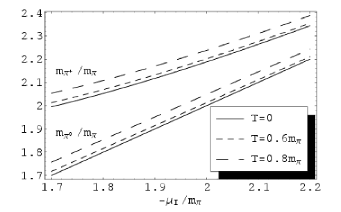
Figure 5.2: $m_{\pi^{0}}$ and $m_{\pi^{+}}$ as a function of high values of the isospin chemical potential at different values of temperature.

In this region, $m_{\pi^{0}}$ increases monotonically both with temperature and chemical potential. $m_{\pi^{+}}$, as the temperature and the chemical potential rise, becomes asymptotically close to $m_{\pi^{0}}$, as was expected (see figure. 5.2). In contrast with the first region, the $\pi^{+}$ mass grows with temperature, and a crossover occurs somewhere in the intermediate region of the chemical potential for the temperature dependence, since near the phase transition point we have $m_{\pi^{+}}(T_{1},\mu_{\mbox{\tiny I}})>m_{\pi^{+}}(T_{2},\mu_{\mbox{\tiny I}})$, and this behavior changes in the high chemical potential region in such a way that $m_{\pi^{+}}(T_{1},\mu_{\mbox{\tiny I}})<m_{\pi^{+}}(T_{2},\mu_{\mbox{\tiny I}})$.

5.2 Condensates

5.2.1 Chiral condensate

The non-vanishing components of the chiral condensate, neglecting higher corrections of order $c^{2}$, are

$$\langle\!\langle J_{s}\rangle\!\rangle_{(1,0)} = -2Bf^{2}c,$$ (5.26)

$$\langle\!\langle J_{s}\rangle\!\rangle_{(1,2)} = Bc\langle\!\langle 0|\pi_{0}^{2}+\tilde{\pi}_{1}^{2}+\tilde{\pi}_{2}^{2}|0\rangle\!\rangle,$$ (5.27)

$$\langle\!\langle J_{s}\rangle\!\rangle_{(3,0)} = -2Bf^{2}\mu_{\mbox{\tiny I}}^{2}c(l_{4}+2\tilde{h}_{1}),$$ (5.28)

keeping the global term $c$. Following the same procedure as in the previous chapters, the chiral condensate at finite temperature and isospin chemical potential is

$$\langle\!\langle\bar{q}q\rangle\!\rangle=-2Bf^{2}c\left\{1+\alpha^{\prime}\left[\bar{l}_{4}+32\pi^{2}\tilde{h}_{1}+2\ln c-4I^{\prime}_{0}-\frac{2}{3}\left(\frac{\pi T}{\mu_{\mbox{\tiny I}}}\right)^{2}\right]\right\}.$$ (5.29)

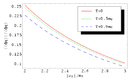
Figure 5.3: Chiral condensate as a function of the isospin chemical potential for different values of the temperature for high values of the chemical potential.

Figure 5.3 shows the chiral condensate behavior at finite temperature for high values of the chemical potential. It continues decreasing with both parameters.

5.2.2 Isospin-number density.

The non-vanishing components of the vector current, within the thermal vacuum, neglecting higher corrections of order $c^{2}$, are

$$\langle\!\langle\bm{V}_{\mu}\rangle\!\rangle_{(1,0)} = -|\mu_{\mbox{\tiny I}}|f^{2}s^{2}u_{\mu}{\bf e}_{3},$$ (5.30)

$$\langle\!\langle\bm{V}_{\mu}\rangle\!\rangle_{(1,2)} = |\mu_{\mbox{\tiny I}}|s^{2}\langle\!\langle 0|\pi_{0}^{2}+\tilde{\pi}_{1}^{2}|0\rangle\!\rangle u_{\mu}{\bf e}_{3},$$ (5.31)

$$\langle\!\langle\bm{V}_{\mu}\rangle\!\rangle_{(3,0)} = -4|\mu_{\mbox{\tiny I}}|^{3}s^{2}(l_{1}+l_{2})u_{\mu}{\bf e}_{3}.$$ (5.32)

The isospin-number density is then

$$\langle\!\langle n_{I}\rangle\!\rangle=-|\mu_{\mbox{\tiny I}}|f^{2}s^{2}\left\{1+2\alpha^{\prime}\left[{\textstyle\frac{1}{3}}\bar{l}_{1}+{\textstyle\frac{2}{3}}\bar{l}_{2}+2\ln c-4I^{\prime}_{0}\right]\right\}.$$ (5.33)

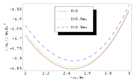
Figure 5.4: Isospin-number density as a function of the isospin chemical potential at different values of the temperature in the high chemical potential limit.

Figure 5.4 shows the isospin-number density for different temperatures and high values of the isospin chemical potential. Due to the logarithmic term, it starts to grow again with the chemical potential. As in the case of the $\pi^{+}$ mass in this high chemical potential limit, it grows with temperature, in contrast to the $|\mu_{\mbox{\tiny I}}|\sim m$ case. A crossover of the different temperature lines must occur somewhere in the intermediate region of the chemical potential.

5.2.3 Pion condensate.

The non-vanishing components of the pseudo-scalar current, within the thermal vacuum and neglecting higher corrections of order $c^{2}$, are

$$\langle\!\langle\bm{J}_{p(1,0)}\rangle\!\rangle = 2Bf^{2}s\tilde{\bf e}_{1},$$ (5.34)

$$\langle\!\langle\bm{J}_{p(1,3)}\rangle\!\rangle = -Bs\langle\!\langle 0|\pi_{0}^{2}+\tilde{\pi}_{1}^{2}+\tilde{\pi}_{2}^{2}\rangle\!\rangle\tilde{\bf e}_{1},$$ (5.35)

$$\langle\!\langle\bm{J}_{p(1,3)}\rangle\!\rangle = 2\mu_{\mbox{\tiny I}}^{2}Bsl_{4}.$$ (5.36)

The pion condensate is then

$$\langle\!\langle\bm{\pi}\rangle\!\rangle=2Bf^{2}s\left\{1+\alpha^{\prime}\left[\bar{l}_{4}+2\ln c-4I^{\prime}_{0}-\left(\frac{\pi T}{\mu_{\mbox{\tiny I}}}\right)^{2}\right]\right\}.$$ (5.37)

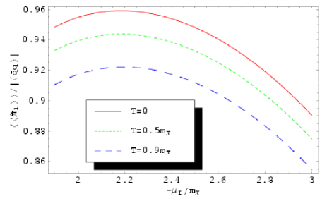
Figure 5.5: Pion condensate as a function of the isospin chemical potential for different temperatures in the limit of high chemical potential.

Figure 5.5 shows the pion condensate at finite temperature and high values of the chemical potential. Like the isospin chemical potential, it has a deflection and starts to decrease, due to the logarithmic terms. Comparing with equation (5.29), if we neglect the term $\tilde{h}_{1}$, the pion condensate and the chiral condensate follow the relation $s\langle\!\langle\bar{q}q\rangle\!\rangle+c\langle\!\langle\tilde{\pi}_{1}\rangle\!\rangle=0$, as was the case in the region $|\mu_{\mbox{\tiny I}}|\gtrsim m$.

Chapter 6 Conclusions

In this thesis, different aspects of pion dynamics within a thermal bath at finite isospin chemical potential were developed in the frame of Chiral Perturbation Theory and Thermo-field Dynamics. The extraction of the pion masses, pion decay constants, and different condensates were analyzed under these conditions in order to get a physical insight about the pion properties in a hot and dense pion gas.

First, an expansion criterion was developed to calculate radiative corrections when the chemical potential becomes bigger than the pion mass (second phase), separating the analysis for the two cases, $|\mu_{\mbox{\tiny I}}|\gtrsim m$ and $|\mu_{\mbox{\tiny I}}|\gg m$. Nevertheless, in our analysis we restrict ourselves to $|\mu_{\mbox{\tiny I}}|\leq m_{\eta}$ in order to avoid strangeness effects. We also considered the so called first phase $|\mu_{\mbox{\tiny I}}|<m$, finding also corrections to masses and decay constants.

Then we calculated the three pion masses at finite temperature and isospin chemical potential. Each of the three masses behaves differently under the introduction of the isospin chemical potential. For values of the chemical potential near the tree-level pion mass, one of the charged pions will condense (in this case, the $\pi^{-}$ when $\mu_{\mbox{\tiny I}}$ becomes negative). The condensation produces a symmetry breaking in the flavor group SU(2)$\rightarrow$U(1), inducing a two-phase structure. However, the thermal bath shifts the condensation point with respect to the tree-level case. It was also possible to extract the decay constants(which now are different for the $\pi^{0}$ and the $\pi^{\pm}$), the chiral condensate and the isospin number density. In the case of the masses, the decay constants and the chiral condensate, it was possible to re define and generalize the G-MOR relation for finite isospin chemical potential.

The fact that the charged pions acquire a shifted mass at zero temperature is a special property of the pions. Except for the charged pion masses, the isospin chemical potential effects appear only for finite temperature; this is also known as the “isospin chemical potential silver blaze problem” [Coh04] which indicates that at zero temperature nothing happens, unless the isospin chemical potential becomes bigger than the pion mass.

Then, we proceed with the consideration of pion masses and condensates for isospin chemical potential values in the vicinity of the transition point. It was possible to find the transition where the $\pi^{-}$ mass vanishes. For a certain temperature $T_{c}$, which depends on $\mu_{\mbox{\tiny I}}$, a normal phase and a condensed phase, as in a superfluid, coexist. With increasing temperature, the thermal $\pi^{-}$ mass grows and thus the pion condensate and the chiral condensate start to decrease. As the temperature and chemical potential increase, the isospin number density (absolute value) grows more rapidly than in the first phase.

Finally, in chapter 5, the pion behavior for the high isospin chemical potential values was studied, obtaining the pion masses and condensates. According to our results, the $\pi^{-}$ normal phase dissappears once again, but this is an artifact of the approximation involved.

A further analysis should include aditional corrections due to higher order diagrams in our expansion parameter. The extension of the present discussion to the strange meson sector could also be interesting to pursue.

Appendix A Expansion in Terms of Pion Fields.

This appendix summarizes the main steps in the construction of the moment expansion of the chiral Lagrangian and currents in both phases. Here we will use the vacuum expectation value in the second phase

$$\bar{U}=e^{i\tilde{\tau}_{1}\varphi}=\cos\varphi+i\tilde{\tau}_{1}\sin\varphi\equiv c+i\tilde{\tau}_{1}s,$$ (A.1)

where for any vector, the $\tilde{\mbox{v}}_{i}$ components refers to the components of the vector rotated in an azimutal angle $\phi$:

$$\tilde{\mbox{v}}_{1}=\mbox{v}_{1}\cos\phi+\mbox{v}_{2}\sin\phi,\qquad\tilde{\mbox{v}}_{2}=-\mbox{v}_{1}\sin\phi+\mbox{v}_{2}\cos\phi,\qquad\tilde{\mbox{v}}_{3}=v_{3}.$$ (A.2)

For the case of the first phase we only have to set $\varphi=0$ (i.e. $c=1$, $s=0$) and $\phi=0$ in all the results of this appendix.

The unitary $U$ fields can be expressed as

$$U=U_{0}+i\bm{\tau}\cdot\bm{U}=U_{0}+i\tilde{\bm{\tau}}\cdot\tilde{\bm{U}},$$ (A.3)

which satisfy the unitarity relation $U_{0}^{2}+\tilde{\bm{U}}^{2}=1$. On the other side, the field $U$ is defined as $U=\bar{U}^{\mbox{\tiny$1/2$}}e^{i\xi}\bar{U}^{\mbox{\tiny$1/2$}}$, with

$$\xi=\bm{\tau}\cdot\bm{\xi}\equiv\bm{\tau}\cdot\frac{\bm{\pi}}{f},\qquad\mbox{and}\qquad\bar{U}^{\mbox{\tiny$1/2$}}=e^{i\tilde{\tau}_{1}\varphi/2}=\cos{\textstyle\frac{\varphi}{2}}+i\tilde{\tau}_{1}\sin{\textstyle\frac{\varphi}{2}}.$$ (A.4)

The exponential can be expanded in terms of the $\xi$ fields. Using the fact that $\xi^{2}=\bm{\xi}^{2}$ we have that

$$e^{i\xi}=\sum_{n=0}\frac{(-\bm{\xi}^{2})^{n}}{(2n)!}+i\xi\sum_{n=0}\frac{(-\bm{\xi}^{2})^{n}}{(2n+1)!}.$$ (A.5)

Now putting the previous equation between the vacuum field $\bar{U}^{\mbox{\tiny$1/2$}}$

$$U=\big{(}c+i\tilde{\tau}_{1}s\big{)}\sum_{n=0}\frac{(-\bm{\xi}^{2})^{n}}{(2n)!}+i\big{(}\xi+is\tilde{\xi}_{1}+(c-1)\tilde{\tau}_{1}\tilde{\xi}_{1}\big{)}\sum_{n=0}\frac{(-\bm{\xi}^{2})^{n}}{(2n+1)!}$$ (A.6)

then

$$U_{0} = c\sum_{n=0}\frac{(-\bm{\xi}^{2})^{n}}{(2n)!}-s\tilde{\xi}_{1}\sum_{n=0}\frac{(-\bm{\xi}^{2})^{n}}{(2n+1)!}$$ (A.7)

$$\tilde{\bm{U}} = s\tilde{\bm{e_{1}}}\sum_{n=0}\frac{(-\bm{\xi}^{2})n}{(2n)!}+\big{(}\bm{\xi}+(c-1)\tilde{\xi}_{1}\tilde{\bm{e_{1}}}\big{)}\sum_{n=0}\frac{(-\bm{\xi}^{2})n}{(2n+1)!}.$$ (A.8)

As we need the terms only up to ${\cal O}(\xi^{4})$, the previous expression reduces to

U_0 &= c-s~ξ_1 -12cξ^2 +16s~ξ_1ξ^2 +124cξ^4
~U = (s +c~ξ_1 -12sξ^2 -16c~ξ_1ξ^2 +124sξ^4)~e_1 +(~ξ_2~e_2 +ξ_3e_3)(1-16ξ^2)
$+$ terms of ${\cal O}(\xi^{5})$.

Another important thing to keep in mind is the fact that the terms $L_{\mu\nu}$ and $R_{\mu\nu}$ vanish for the values of the external fields $v={\textstyle\frac{1}{2}}\mu_{\mbox{\tiny I}}\tau_{3}u$ and $a=0$.

A.1 Expansion of the Chiral Lagrangian

The lagrangian with massive quarks at finite isospin chemical potential is

$${\cal L}_{2}(M,0,{\textstyle\frac{1}{2}}\mu_{\mbox{\tiny I}}\tau_{3}u,0) = \frac{f^{2}}{4}Tr\left[(D_{\mu}U)^{\dagger}D^{\mu}U+2BM(U^{\dagger}+U)\right]$$ (A.9)

$${\cal L}_{4}(M,0,{\textstyle\frac{1}{2}}\mu_{\mbox{\tiny I}}\tau_{3}u,0) = {\textstyle\frac{1}{4}}l_{1}\left(Tr\left[(D_{\mu}U)^{\dagger}D^{\mu}U\right]\right)^{2}$$

$$+{\textstyle\frac{1}{4}}l_{2}Tr\left[(D_{\mu}U)^{\dagger}D_{\nu}U\right]Tr\left[(D^{\mu}U)^{\dagger}D^{\nu}U\right]$$

$$+{\textstyle\frac{1}{4}}(l_{3}+l_{4})\left(Tr\left[BM(U^{\dagger}+U)\right]\right)^{2}$$

$$+{\textstyle\frac{1}{4}}l_{4}Tr\left[(D_{\mu}U)^{\dagger}D^{\mu}U\right]Tr\left[BM(U^{\dagger}+U)\right]$$

$$-{\textstyle\frac{1}{4}}l_{7}\left(Tr\left[BM(U^{\dagger}-U)\right]\right)^{2}$$

$$+\mbox{constants}$$

with the covariant derivative

$$DU=\partial U-i\mu_{\mbox{\tiny I}}u[{\textstyle\frac{1}{2}}\tau_{3},U]=\partial U_{0}+i\bm{\tau}\cdot(\partial\bm{U}-\mu_{\mbox{\tiny I}}u\bm{U}\times\bm{e_{3}})$$ (A.11)

First of all, we need to compute the traces. It is enough to calculate the traces of the main structures of the Lagrangian: $Tr[(D_{\mu}U)^{\dagger}D_{\nu}U]$, $Tr[M(U^{\dagger}+U)]$, and $Tr[M(U^{\dagger}+U)]^{2}$.

Using the shape of the covariat derivative in Eq. (A.11)

$$Tr\left[(D_{\mu}U)^{\dagger}D_{\nu}U\right] = Tr\left[\left\{\partial_{\mu}U_{0}-i\bm{\tau}\cdot(\partial_{\mu}\bm{U}-\mu_{\mbox{\tiny I}}u_{\mu}\tilde{\bm{U}}\times\bm{e_{3}})\right\}\Big{\{}h.c.,\quad\mu\leftrightarrow\nu\Big{\}}\right]$$ (A.12)

$$= 2\big{[}\partial_{\mu}U_{0}\partial_{\nu}U_{0}+(\partial_{\mu}\bm{U}-\mu_{\mbox{\tiny I}}u_{\mu}\bm{U}\times\bm{e_{3}})\cdot(\mu\rightarrow\nu)\big{]}$$

$$= 2\big{[}\partial_{\mu}U_{0}\partial_{\nu}U_{0}+\partial_{\mu}\bm{U}\cdot\partial_{\mu}\bm{U}+\mu_{\mbox{\tiny I}}^{2}(\tilde{U}_{1}^{2}+\tilde{U}_{2}^{2})u_{\mu}u_{\nu}$$

$$\hskip 56.9055pt+\mu_{\mbox{\tiny I}}(\{\tilde{U}_{1}\partial_{\nu}\tilde{U}_{2}-\tilde{U}_{2}\partial_{\nu}\tilde{U}_{1}\}u_{\mu}+\mu\leftrightarrow\nu)\big{]}.$$

Now, using the fact that

$$BM=B\big{[}{\textstyle\frac{1}{2}}(m_{u}+m_{d})+{\textstyle\frac{1}{2}}(m_{u}-m_{d})\tau_{3}\big{]}={\textstyle\frac{1}{2}}m^{2}(1+\epsilon_{ud}\tau_{3}),$$ (A.13)

the other terms we want to calculate are

$$Tr\left[BM(U^{\dagger}+U)\right] = Tr\left[2BMU_{0}\right]=2m^{2}U_{0}$$ (A.14)

$$Tr\left[BM(U^{\dagger}-U)\right]^{2} = Tr\left[-2iBM\bm{\tau}\cdot\bm{U}\right]^{2}=-4m^{4}\epsilon_{ud}^{2}U_{3}^{2}.$$ (A.15)

A.1.1 ${\cal L}_{2}$ up to order $\pi^{4}$

Now we are going to expand the the structures that appear in ${\cal L}_{2}$, $Tr[(D_{\mu}U)^{\dagger}D^{\mu}U]$ and $Tr[M(U^{\dagger}+U)]$, neglecting higher terms of ${\cal O}(\xi^{5})$. From Eq. (A.12)

$$Tr\left[(D_{\mu}U)^{\dagger}D^{\mu}U\right]=2\big{[}(\partial U_{0})^{2}+(\partial\bm{U})^{2}+2\mu_{\mbox{\tiny I}}(\tilde{U}_{1}\partial_{0}\tilde{U}_{2}-\tilde{U}_{2}\partial_{0}\tilde{U}_{1})+\mu_{\mbox{\tiny I}}^{2}(\tilde{U}_{1}^{2}+\tilde{U}_{2}^{2})\big{]}.$$ (A.16)

Using the results of Eqs. (A) and (A)

$$(\partial U_{0})^{2}+(\partial\tilde{\bm{U}})^{2} = (\partial\bm{\xi})^{2}-{\textstyle\frac{1}{3}}(\partial\bm{\xi})^{2}\bm{\xi}^{2}+{\textstyle\frac{1}{3}}(\bm{\xi}\cdot\partial\bm{\xi})^{2}$$ (A.17)

$$\tilde{U}_{1}\partial_{0}\tilde{U}_{2}-\tilde{U}_{2}\partial_{0}\tilde{U}_{1} = s\partial_{0}\tilde{\xi}_{2}+c(\tilde{\xi}_{1}\partial_{0}\tilde{\xi}_{2}-\tilde{\xi}_{2}\partial_{0}\tilde{\xi}_{1})-{\textstyle\frac{2}{3}}s(\partial_{0}\tilde{\xi}_{2}\bm{\xi}^{2}-\tilde{\xi}_{2}\bm{\xi}\cdot\partial_{0}\bm{\xi})$$ (A.18)

$$-{\textstyle\frac{1}{3}}c(\tilde{\xi}_{1}\partial_{0}\tilde{\xi}_{2}-\tilde{\xi}_{2}\partial_{0}\tilde{\xi}_{1})\bm{\xi}^{2}$$

$$\tilde{U}_{1}^{2}+\tilde{U}_{2}^{2} = s^{2}+2cs\tilde{\xi}_{1}+c^{2}\tilde{\xi}_{1}^{2}+\tilde{\xi}_{2}^{2}-s^{2}\bm{\xi}^{2}$$ (A.19)

$$-{\textstyle\frac{4}{3}}cs\tilde{\xi}_{1}\bm{\xi}^{2}-{\textstyle\frac{1}{3}}(c^{2}\tilde{\xi}_{1}^{2}+\tilde{\xi}_{2}^{2}-s^{2}\bm{\xi}^{2})\bm{\xi}^{2}.$$

Even though we neglect constants and total derivative terms in the lagrangian, we will keep them in the previous equation for further considerations in ${\cal L}_{4}$.

For the case of $Tr[M(U^{\dagger}+U)]$, from Eq. (A.14), we just need to replace the results of Eq. (A).

A.1.2 ${\cal L}_{4}$ up to order $\pi^{2}$

In the next part, the structures of the ${\cal L}_{4}$ Lagrangian will be expanded in order of apparition from Eq. (A.1), neglecting higher terms of ${\cal O}(\xi^{3})$. In this case the resulting constant terms and total derivative terms will be neglected, since they do not contribute. It will be used also the fact that $\tilde{\xi}_{1}\partial_{0}\tilde{\xi}_{2}=-\tilde{\xi}_{2}\partial_{0}\tilde{\xi}_{1}$ + a total derivative.

Using the results of Eqs. (A.16)-(A.19) up to order $\xi^{2}$

$$Tr\left[(D_{\mu}U)^{\dagger}D^{\mu}U\right]^{2} = 4\big{[}(\partial\bm{\xi})^{2}-{\textstyle\frac{1}{3}}(\partial\bm{\xi})^{2}+2\mu_{\mbox{\tiny I}}\{s\partial_{0}\tilde{\xi}_{2}+c(\tilde{\xi}_{1}\partial_{0}\tilde{\xi}_{2}-\tilde{\xi}_{2}\partial_{0}\tilde{\xi}_{1})\}$$

$$+\mu_{\mbox{\tiny I}}^{2}[s^{2}+2cs\tilde{\xi}_{1}-s^{2}\bm{\xi}^{2}+c^{2}\tilde{\xi}_{1}^{2}]\big{]}^{2}$$

$$= 8\mu_{\mbox{\tiny I}}^{2}s^{2}\big{[}2\mu_{\mbox{\tiny I}}^{2}cs\tilde{\xi}_{1}+(\partial\bm{\xi})^{2}+2(\partial_{0}\tilde{\xi}_{2})^{2}+8\mu_{\mbox{\tiny I}}c\tilde{\xi}_{1}\partial_{0}\tilde{\xi}_{2}$$

$$\qquad-\mu_{\mbox{\tiny I}}^{2}s^{2}\bm{\xi}^{2}+3\mu_{\mbox{\tiny I}}^{2}c^{2}\tilde{\xi}_{1}^{2}+\mu_{\mbox{\tiny I}}^{2}\tilde{\xi}_{2}^{2}\big{]}$$

$$+{\cal O}(\xi^{3})+\mbox{tot. deriv.}+\mbox{const.}$$

Using Eq. (A.12) and inserting Eqs. (A) and (A) up to order $\xi^{2}$

$$Tr\left[(D_{\mu}U)^{\dagger}D_{\nu}U\right]^{2} = 4\big{[}\partial_{\mu}\bm{\xi}\cdot\partial_{\nu}\bm{\xi}+\mu_{\mbox{\tiny I}}^{2}\{s^{2}+2cs\tilde{\xi}_{1}+c^{2}\tilde{\xi}_{1}^{2}+\tilde{\xi}_{2}^{2}-s^{2}\bm{\xi}^{2}\}u_{\mu}u_{\nu}$$

$$+\mu_{\mbox{\tiny I}}\{[s\partial_{\mu}\tilde{\xi}_{2}+c(\tilde{\xi}_{1}\partial_{\mu}\tilde{\xi}_{2}-\tilde{\xi}_{2}\partial_{\mu}\tilde{\xi}_{1})]u_{\nu}+\mu\leftrightarrow\nu\}\big{]}^{2}$$

$$= 8\mu_{\mbox{\tiny I}}^{2}s^{2}\big{[}2\mu_{\mbox{\tiny I}}^{2}cs\tilde{\xi}_{1}+(\partial_{0}\bm{\xi})^{2}+(\partial\tilde{\xi}_{2})^{2}+(\partial_{0}\tilde{\xi}_{2})^{2}$$

$$\qquad+8\mu_{\mbox{\tiny I}}c\tilde{\xi}_{1}\partial_{0}\tilde{\xi}_{2}+\mu_{\mbox{\tiny I}}^{2}(3c^{2}\tilde{\xi}_{1}^{2}+\tilde{\xi}_{2}^{2}-s^{2}\bm{\xi}^{2})\big{]}$$

$$+{\cal O}(\xi^{3})+\mbox{tot. deriv.}+\mbox{const.}$$

From Eq. (A.14) and Eq. (A) up to order $\xi^{2}$

$$Tr\left[BM(U^{\dagger}+U)\right] = 4m^{4}\left[c-s\tilde{\xi}_{1}-{\textstyle\frac{1}{2}}c\bm{\xi}^{2}\right]^{2}$$ (A.22)

$$= -4m^{4}\left[2cs\tilde{\xi}_{1}+c^{2}\bm{\xi}^{2}-s^{2}\tilde{\xi}_{1}^{2}\right]+{\cal O}(\xi^{3})+\mbox{const.}$$

From Eqs. (A.16)-(A.19), Eq. (A.14) and Eq. (A) up to order $\xi^{2}$

$$Tr\left[(D_{\mu}U)^{\dagger}D^{\mu}U\right]Tr\left[BM(U^{\dagger}+U)\right]$$

$$\qquad=4m^{2}[(\partial\bm{\xi})^{2}+2\mu_{\mbox{\tiny I}}\{s\partial_{0}\tilde{\xi}_{2}+c(\tilde{\xi}_{1}\partial_{0}\tilde{\xi}_{2}-\tilde{\xi}_{2}\partial_{0}\tilde{\xi}_{1})\}$$

$$\qquad\qquad\quad+\mu_{\mbox{\tiny I}}^{2}\{s^{2}+2cs\tilde{\xi}_{1}+c^{2}\tilde{\xi}_{1}^{2}+\tilde{\xi}_{2}^{2}-s^{2}\bm{\xi}^{2}\}][c-s\tilde{\xi}_{1}-{\textstyle\frac{1}{2}}c\bm{\xi}^{2}]$$

$$\qquad=-4m^{2}[\mu_{\mbox{\tiny I}}^{2}s(1-3c^{2})\tilde{\xi}_{1}+2\mu_{\mbox{\tiny I}}(1-3c^{2}\tilde{\xi}_{1}\partial_{0}\tilde{\xi}_{2}-c(\partial\bm{\xi})^{2}$$

$$\qquad\qquad\qquad+\mu_{\mbox{\tiny I}}^{2}c\{{\textstyle\frac{3}{2}}s^{2}\bm{\xi}^{2}-(1-3s^{2})\tilde{\xi}_{1}^{2}+\tilde{\xi}_{2}^{2}\}]$$ (A.23)

$$\qquad\quad+{\cal O}(\xi^{3})+\mbox{tot. deriv.}+\mbox{const.}$$

From Eqs. (A.15) and (A) up to order $\xi^{2}$

$$Tr\left[BM(U^{\dagger}-U)\right]^{2}=-4M^{4}\epsilon_{ud}^{2}\xi_{3}^{2}+{\cal O}(\xi^{3})$$ (A.24)

A.2 Expansion of currents

In this section the currents that will be used in this thesis to obtain information on condensates and on the decay constant will be expand in terms of pion fields.

The currents are sorted in powers of momentum

$$J=J_{(1)}+J_{(3)}+\cdots$$ (A.25)

For the case of the PCAC relation, we need to expand the axial current up to order $\pi^{3}$ in $A_{(1)}$ and order $\pi$ in $A_{(3)}$. As this relation will be used only in the first phase, it will be calculated only with the values $c=1$ and $s=0$. So, the effective axial current will be of the form

$$A_{\mbox{\small eff}}=A_{(1,1)}+A_{(1,3)}+A_{(3,1)}$$ (A.26)

For the case of currents that will be used in the calculation of condensates, an expansion will be developed in the second phase as I did the previous section,. In the case of the first phase, we just need to take the terms $c=1$ and $s=0$.

For one loop corrections to the condensates, we need to expand up to order $\pi^{2}$ in $J_{(1)}$ and order zero in $J_{(3)}$ according to the power counting in chapter 1.1.2. The effective current in this case will be

$$J_{\mbox{\small eff}}=J_{(1,0)}+J_{(1,1)}+J_{(1,2)}+J_{(3,0)},$$ (A.27)

and then, the respective condensate is

$$\langle\!\langle J\rangle\!\rangle=\langle\!\langle 0|J_{(1,0)}|0\rangle\!\rangle+\langle\!\langle 0|J_{(1,2)}|0\rangle\!\rangle+\langle\!\langle 0|J_{(3,0)}|0\rangle\!\rangle.$$ (A.28)

A.2.1 Axial current.

As was said before, we need the axial current in the first phase, to get, via the PCAC relation, the pion decay constant. Since it will be saturated with a single pion, we need to expand it up to order $(\pi)^{3}$. The axial current for massive quarks at finite chemical potential is

$$A_{\mu}^{a}=\frac{\delta S_{\chi}}{\delta a_{\mu}^{a}}(M,0,{\textstyle\frac{1}{2}}\mu_{\mbox{\tiny I}}u\tau_{3},0).$$ (A.29)

The expressions for $A_{(1)}$ and $A_{(3)}$ with finite quark masses and finite chemical potential are

$$A_{(1)\mu}^{a} = \frac{f^{2}}{4}Tr\left[i\big{\{}{\textstyle\frac{1}{2}}\tau^{a},U^{\dagger}\big{\}}D^{\mu}U~{}+h.c.\right]$$ (A.30)

$$A_{(3)\mu}^{a} = {\textstyle\frac{1}{2}}l_{1}Tr\left[i\big{\{}{\textstyle\frac{1}{2}}\tau^{a},U^{\dagger}\big{\}}D^{\mu}U~{}+h.c.\right]Tr\left[(D_{\alpha}U)^{\dagger}D^{\alpha}U\right]$$ (A.31)

$$+{\textstyle\frac{1}{2}}l_{2}Tr\left[i\big{\{}{\textstyle\frac{1}{2}}\tau^{a},U^{\dagger}\big{\}}D_{\beta}U\delta^{\mu}_{\alpha}~{}+h.c.,~{}\alpha\leftrightarrow\beta\right]Tr\left[(D^{\alpha}U)^{\dagger}D^{\beta}U\right]$$

$$+{\textstyle\frac{1}{4}}l_{4}Tr\left[i\big{\{}{\textstyle\frac{1}{2}}\tau^{a},U^{\dagger}\big{\}}D^{\mu}U~{}+h.c.\right]Tr\left[BM(U^{\dagger}+U)\right].$$

First we need to calculate the trace of the following term

$$Tr\left[i\big{\{}{\textstyle\frac{1}{2}}\tau^{a},U^{\dagger}\big{\}}DU\right] = Tr\left[\big{\{}i\tau^{a}U_{0}+U^{a}\big{\}}\big{\{}\partial U_{0}+i\bm{\tau}\cdot[\partial\bm{U}-\mu_{\mbox{\tiny I}}u\bm{U}\times{\bf e}_{3}]\big{\}}\right]$$ (A.32)

$$= 2\left[\bm{U}\partial U_{0}-U_{0}\partial\bm{U}+\mu_{\mbox{\tiny I}}uU_{0}\bm{U}\times{\bf e}_{3}\right]^{a}.$$

Using the expansion of the fields in equations (A) and (A) up to order $\xi^{3}$ with $c=1$ and $s=0$ we get

$$Tr\left[i\big{\{}{\textstyle\frac{1}{2}}\bm{\tau},U^{\dagger}\big{\}}DU\right]=-2\left[\partial\bm{\xi}-\mu_{\mbox{\tiny I}}u\bm{\xi}\times{\bf e}_{3}\right]\left[1-{\textstyle\frac{2}{3}}\bm{\xi}^{2}\right]-{\textstyle\frac{4}{3}}\bm{\xi}(\bm{\xi}\cdot\partial\bm{\xi}).$$ (A.33)

This expression starts with terms of order $\xi$. In the case of $A_{(3)}$, we need just expressions up to order $\xi$, but from equation (A.12) we can see that the term $Tr\big{[}(D_{\mu}U)^{\dagger}D_{\nu}U\big{]}$ is of order $\xi^{2}$. Then we can neglect the terms proportional to $l_{1}$ and $l_{2}$, and using eq. (A.14) we obtain

$$\bm{A}_{(1)} = -f^{2}\left\{\left[\partial\bm{\xi}-\mu_{\mbox{\tiny I}}u\bm{\xi}\times{\bf e}_{3}\right]\left[1-{\textstyle\frac{2}{3}}\bm{\xi}^{2}\right]+{\textstyle\frac{2}{3}}\bm{\xi}(\bm{\xi}\cdot\partial\bm{\xi})\right\}$$ (A.34)

$$\bm{A}_{(3)} = -2l_{4}m^{2}\left[\partial\bm{\xi}-\mu_{\mbox{\tiny I}}u\bm{\xi}\times{\bf e}_{3}\right]$$ (A.35)

A.2.2 Scalar current.

We need the scalar current to calculate radiative corrections to the quark condensate (or chiral condensate) defined as

$$\langle\!\langle\bar{q}q\rangle\!\rangle\equiv\langle\!\langle 0|\bar{q}q|0\rangle\!\rangle=\langle\!\langle 0|J_{s}|0\rangle\!\rangle$$ (A.36)

The scalar current for massive quarks and finite isospin chemical potential is

$$J_{s}=-\frac{\delta S\chi}{\delta s^{0}}(M,0,{\textstyle\frac{1}{2}}\mu_{\mbox{\tiny I}}u\tau_{3},0).$$ (A.37)

The expressions for $J_{s(1)}$ and $J_{s(3)}$ with finite quark masses and finite chemical potential are

$$J_{s(1)} = -{\textstyle\frac{1}{2}}f^{2}BTr\big{[}U^{\dagger}+U\big{]}$$ (A.38)

$$J_{s(3)} = -{\textstyle\frac{1}{2}}(l_{3}+l_{4})BTr\big{[}U^{\dagger}+U\big{]}Tr\big{[}BM(U^{\dagger}+U)\big{]}$$

$$-{\textstyle\frac{1}{4}}l_{4}BTr\big{[}(D_{\mu}U)^{\dagger}D^{\mu}U\big{]}Tr\big{[}U^{\dagger}+U\big{]}$$

$$-4\tilde{h}_{1}BTr\big{[}BM\big{]}$$

For $J_{s(2)}$, expanded up to oreder $(\pi)^{2}$, we use the results of equation (A)

$$J_{s(1)}=-2f^{2}BU_{0}=-2f^{2}B\left(c-s\tilde{\xi}_{1}-{\textstyle\frac{1}{2}}c\bm{\xi}^{2}\right)$$ (A.40)

$J_{s(3)}$ at order $(\pi)^{0}$ is just setting the fields $U=\bar{U}$. Then using the equation (A.16), with $\bar{U}=c+i\tilde{\tau}_{1}s$

$$J_{s(3,0)} = -4(l_{3}+l_{4})Bm^{2}\bar{U}_{0}^{2}-2l_{4}B\mu_{\mbox{\tiny I}}^{2}(\tilde{\bar{U}}_{1}^{2}+\tilde{\bar{U}}_{2}^{2})\bar{U}_{0}-4\tilde{h}_{1}Bm^{2}$$ (A.41)

$$= -2B\big{[}2(l_{3}+l_{4})m^{2}c^{2}+l_{4}\mu_{\mbox{\tiny I}}^{2}s^{2}c+2\tilde{h}_{1}m^{2}\big{]}.$$

A.2.3 Vector current.

The vector current will be used to calculate the isospin number density condensate, where

$$\langle\!\langle n_{I}\rangle\!\rangle\equiv\langle\!\langle 0|{\textstyle\frac{1}{2}}q^{\dagger}\tau_{3}q|0\rangle\!\rangle=\langle\!\langle 0|V_{0}^{3}|0\rangle\!\rangle.$$ (A.42)

The pseudo-scalar current for massive quarks at finite isospin chemical potential is

$$V_{\mu}^{a}=\frac{\delta S_{\chi}}{\delta v_{\mu}^{a}}(M,0,{\textstyle\frac{1}{2}}\mu_{\mbox{\tiny I}}u\tau_{3},0)$$ (A.43)

The expressions for $V_{(1)\mu}^{a}$ and $V_{(3)_{\mu}}^{a}$ are

$$V_{(1)\mu}^{a} = \frac{f^{2}}{4}Tr\left[-i\big{[}{\textstyle\frac{1}{2}}\tau^{a},U^{\dagger}\big{]}D^{\mu}U~{}+h.c.\right]$$ (A.44)

$$V_{(3)\mu}^{a} = {\textstyle\frac{1}{2}}l_{1}Tr\left[-i\big{[}{\textstyle\frac{1}{2}}\tau^{a},U^{\dagger}\big{]}D^{\mu}U~{}+h.c.\right]Tr\left[(D_{\alpha}U)^{\dagger}D^{\alpha}U\right]$$ (A.45)

$$+{\textstyle\frac{1}{2}}l_{2}Tr\left[-i\big{[}{\textstyle\frac{1}{2}}\tau^{a},U^{\dagger}\big{]}D_{\beta}U\delta^{\mu}_{\alpha}~{}+h.c.,~{}\alpha\leftrightarrow\beta\right]Tr\left[(D^{\alpha}U)^{\dagger}D^{\beta}U\right]$$

$$+{\textstyle\frac{1}{4}}l_{4}Tr\left[-i\big{[}{\textstyle\frac{1}{2}}\tau^{a},U^{\dagger}\big{]}D^{\mu}U~{}+h.c.\right]Tr\left[BM(U^{\dagger}+U)\right]$$

First we need to calculate the trace of the following term

$$Tr\left[-i\big{[}{\textstyle\frac{1}{2}}\tau^{2},U^{\dagger}\big{]}DU\right] = Tr\left[-i\big{(}\bm{U}\times\bm{\tau}\big{)}^{a}\big{\{}\partial U_{0}+i\bm{\tau}\cdot[\partial\bm{U}-\mu_{\mbox{\tiny I}}u\bm{U}\times{\bf e}_{3}]\big{\}}\right]$$ (A.46)

$$= 2\left[\bm{U}\times\partial\bm{U}-\mu_{\mbox{\tiny I}}u\bm{U}\times\big{(}\bm{U}\times{\bf e}_{3}\big{)}\right]^{a}$$

Expanding up to order $\xi^{2}$

$$Tr\left[-i\big{[}{\textstyle\frac{1}{2}}\bm{\tau},U^{\dagger}\big{]}DU\right]$$

$$\quad=2\left[-\mu_{\mbox{\tiny I}}s\xi_{3}u+\tilde{\xi}_{2}\partial\xi_{3}-\xi_{3}\partial\tilde{\xi}_{2}-\mu_{\mbox{\tiny I}}c\tilde{\xi}_{1}\xi_{3}\right]\tilde{\bf e}_{1}$$

$$\qquad+2\left[-s\partial\tilde{\xi}_{2}+c\xi_{3}\partial\tilde{\xi}_{1}-c\tilde{\xi}_{1}\partial\xi_{3}-\mu_{\mbox{\tiny I}}\tilde{\xi}_{2}\xi_{3}u\right]\tilde{\bf e}_{2}$$

$$\qquad+2\Big{[}\mu_{\mbox{\tiny I}}s^{2}u+2\mu_{\mbox{\tiny I}}cs\tilde{\xi}_{1}u+s\partial\tilde{\xi}_{2}+c\tilde{\xi}_{1}\partial\tilde{\xi}_{2}-c\tilde{\xi}_{2}\partial\tilde{\xi}_{1}$$ (A.47)

$$\hskip 142.26378pt-\mu_{\mbox{\tiny I}}\left(s^{2}\bm{\xi}^{2}-c^{2}\tilde{\xi}_{1}^{2}-\tilde{\xi}_{2}^{2}\right)u\Big{]}{\bf e}_{3},$$

we see that we only need to replace it to obtain $V_{(1)\mu}^{a}$ up to order $\xi^{2}$. For the case of $V_{(3,0)\mu}^{a}$ we only need to set $\xi=0$. Using equation (A.14) and (A.12), we get

$$\bm{V}_{(3,0)\mu}=2s^{2}\left[2\mu_{\mbox{\tiny I}}^{2}s^{2}(l_{1}+l_{2})+m^{2}l_{4}\right]{\bf e}_{3}u_{\mu}.$$ (A.48)

A.2.4 Pseudo-scalar current.

The pseudo-scalar current will be used to calculate the pion condensate, where

$$\langle\!\langle\pi^{a}\rangle\!\rangle\equiv\langle\!\langle 0|{\textstyle\frac{1}{2}}i\bar{q}\gamma_{5}\tau^{a}q|0\rangle\!\rangle=\langle\!\langle 0|J_{p}^{a}|0\rangle\!\rangle.$$ (A.49)

The pseudo-scalar current for massive quarks at finite isospin chemical potential is

$$J_{p}^{a}=\frac{\delta S_{\chi}}{\delta p^{a}}(M,0,{\textstyle\frac{1}{2}}\mu_{\mbox{\tiny I}}u\tau_{3},0)$$ (A.50)

The expressions for $J_{p(1)}^{a}$ and $J_{p(3)}^{a}$ are

$$J_{p(1)}^{a} = {\textstyle\frac{1}{2}}f^{2}BTr\left[i\tau^{a}(U^{\dagger}-U)\right]$$ (A.51)

$$J_{p(3)}^{a} = {\textstyle\frac{1}{2}}(l_{3}+l_{4})BTr\left[i\tau^{a}(U^{\dagger}-U)\right]Tr\left[BM(U^{\dagger}+U)\right]$$ (A.52)

$$+{\textstyle\frac{1}{4}}l_{4}BTr\left[i\tau^{a}(U^{\dagger}-U)\right]Tr\left[(D_{\mu}U)^{\dagger}D^{\mu}U\right].$$

Considering

$$Tr\left[i\tau^{a}(U^{\dagger}-U)\right]=2U^{a},$$ (A.53)

then the expansion of $J_{p(1)}^{a}$ up to order $\xi^{2}$ corresponds just to re placethe expansion of $U^{a}$ (eq. (A) and $J_{p(3,0)}^{a}$ replacing the previous equation, equation (A.14) and (A.12) with $\xi=0$

$$\bm{J}_{p(1)} = 2Bf^{2}\left[\left(s+c\tilde{\xi}_{1}-{\textstyle\frac{1}{2}}s\bm{\xi}^{2}\right)\tilde{\bf e}_{1}+\tilde{\xi}_{2}\tilde{\bf e}_{2}+\xi_{3}{\bf e}_{3}+{\cal O}(\xi^{3})\right]$$ (A.54)

$$\bm{J}_{p(3,0)} = 2Bs\left[2m^{2}c(l_{3}+l_{4})+\mu_{\mbox{\tiny I}}^{2}s^{2}l_{4}\right]\tilde{\bf e}_{1}$$ (A.55)

Appendix B Some useful formulas, identities and constants

B.1 $l_{i}$ constants

The $\bar{l}_{i}$ coupling constants are defined as the value of the corresponding couplings at the scale $\Lambda=m$, subtracting the divergent part proportional to $\lambda$:

$$l_{i}(\Lambda)=\frac{\gamma_{i}}{32\pi^{2}}\left[\bar{l}_{i}+\ln\frac{m^{2}}{\Lambda^{2}}-\lambda\right],$$ (B.1)

with

$$\lambda=\frac{2}{4-d}+\ln 4\pi+\Gamma^{\prime}(1)+1$$ (B.2)

for $i=1,\dots,6$. The table B.1 was obtained from [Sch02]; it shows the different $l_{i}(\Lambda)$ and $l_{7}$ constants evaluated at the scale $\Lambda=m$, the corresponding $\gamma_{i}$ factors and indicates also from which processes they where obtained. The other constants, $\tilde{h}_{i}$, that appear in the chiral ${\cal L}_{4}$ Lagrangian, are model dependent and do not involve divergences.

$\bar{l}_{i}$	Value	Obtained from	$\gamma_{i}$
	$-2.23\pm 3.7$ [GL84]	$\pi\pi$ D-wave scattering lengths ${\cal O}(P^{4})$
	$-1.7\pm 1.0$ [BCG94]	$\pi\pi$ and $K_{l4}$
$\bar{l}_{1}$	$-1.5$ [BCE+97]	$\pi\pi$ D-wave scattering lengths ${\cal O}(P^{6})$	$1/3$
	$-1.8$ [CGL01]	$\pi\pi$ scattering ${\cal O}(P^{4})$ + Roy equations
	$-0.4\pm 0.6$ [CGL01]	$\pi\pi$ scattering ${\cal O}(P^{6})$ + Roy equations
	$6.03\pm 1.3$ [GL84]	$\pi\pi$ D-wave scattering lengths ${\cal O}(P^{4})$
	$6.1\pm 0.5$ [BCG94]	$\pi\pi$ and $K_{l4}$
$\bar{l}_{2}$	$4.5$ [BCE+97]	$\pi\pi$ D-wave scattering lengths ${\cal O}(P^{6})$	$2/3$
	$5.4$ [CGL01]	$\pi\pi$ scattering ${\cal O}(P^{4})$ + Roy equations
	$4.3\pm 0.1$ [CGL01]	$\pi\pi$ scattering ${\cal O}(P^{6})$ + Roy equations
	$2.9\pm 2.4$ [GL84]	SU(3) mass formulae
$\bar{l}_{3}$	$|\bar{l}_{3}|<16$ [CGL01]	$K_{l4}$ decay	$-1/2$
	$4.3\pm 0.9$ [GL84]	$F_{K}/F_{\pi}$
$\bar{l}_{4}$	$4.4\pm 0.3$ [BCT98]	scalar form factor ${\cal O}(P^{6})$	2
	$4.4\pm 0.2$ [CGL01]	$\pi\pi$ scattering ${\cal O}(P^{6})$ + Roy equations
	$13.9\pm 1.3$ [GL84]	$\pi\rightarrow e\nu\gamma$ ${\cal O}(P^{4})$
$\bar{l}_{5}$	$13.0\pm 0.9$ [BCT98]	$\pi\rightarrow e\nu\gamma$ ${\cal O}(P^{6})$	$-1/6$
	$16.5\pm 1.1$ [GL84]	$\langle r^{2}\rangle_{\pi}$ ${\cal O}(P^{4})$
$\bar{l}_{6}$	$16.0\pm 0.5\pm 0.7$ [BCT98]	vector form factor ${\cal O}(P^{6})$	$-1/3$
$l_{7}$	$\sim 5\times 10^{-3}$ [GL84]	$\pi^{0}-\eta$ mixing	0

Table B.1: $l_{i}$ constants values.

B.2 $f$, $B$ and $\epsilon_{ud}$.

The one-loop corrections for the pion mass and the pion decay constant are

$$m_{\pi} = m[1-\alpha\bar{l}_{3}/4]~{}~{}\approx~{}~{}139.57~{}\mbox{MeV}$$ (B.3)

$$f_{\pi} = f[1+\alpha\bar{l}_{4}]~{}~{}\approx~{}~{}92.42~{}\mbox{MeV},$$ (B.4)

with $\alpha=(m/4\pi f)^{2}$. From these definitions and with the value of $\bar{l}_{3}$ and $\bar{l}_{4}$ it is easy to derive the value of the tree-level pion mass and decay constant.

$$\alpha \approx 0.017$$ (B.5)

$$m \approx 141~{}\mbox{MeV}$$ (B.6)

$$f \approx 86~{}\mbox{MeV}.$$ (B.7)

From the definition of the tree-level mass, $m^{2}=B(m_{u}+m_{d})$, using the current-quark masses values we can extract the value of $B$

$$m_{u}+m_{d}=5~{}\mbox{to}~{}11~{}\mbox{MeV}\qquad\Longrightarrow\qquad B\approx 1.8~{}\mbox{to}~{}4~{}\mbox{GeV}$$ (B.8)

From the value of the light quark mass ratios, we can evaluate the $\epsilon_{ud}$ constant

$$\frac{m_{u}}{m_{d}}=0.2~{}\mbox{to}~{}0.7\qquad\Longrightarrow\qquad\epsilon_{ud}=\frac{m_{u}-m_{d}}{m_{u}+m_{d}}=-0.2~{}\mbox{to}~{}-0.7$$ (B.9)

B.3 Functions and definitions

The functions involved in the radiative corrections in the first phase are

$$\alpha = (m/4\pi f)^{2}$$ (B.10)

$$\underline{\lambda} = \lambda-\ln(m^{2}/\Lambda^{2})$$ (B.11)

$$I = \int_{1}^{\infty}dx\sqrt{x^{2}-1}[n_{B}(mx-|\mu_{\mbox{\tiny I}}|)+n_{B}(mx+|\mu_{\mbox{\tiny I}}|)]$$ (B.12)

$$J = \int_{1}^{\infty}dxx\sqrt{x^{2}-1}[n_{B}(mx-|\mu_{\mbox{\tiny I}}|)-n_{B}(mx+|\mu_{\mbox{\tiny I}}|)]$$ (B.13)

$$I_{n} = \int_{1}^{\infty}dxx^{2n}\sqrt{x^{2}-1}~{}2n_{B}(mx)$$ (B.14)

being $\alpha$ the perturbative parameter. These integrals do not depend on the chemical potential sign, and grow with both, temperature and chemical potential

In the case of the second phase, we denote the same functions with a prime: $\alpha^{\prime}$, $I^{\prime}$, $J^{\prime}$, $I^{\prime}_{n}$ which are the same functions, but with $|\mu_{\mbox{\tiny I}}$ instead of $m$.

$$\alpha^{\prime} = (\mu_{\mbox{\tiny I}}/4\pi f)^{2}$$ (B.15)

$$\underline{\lambda}^{\prime} = \lambda-\ln(\mu_{\mbox{\tiny I}}^{2}/\Lambda^{2})$$ (B.16)

$$I^{\prime} = \int_{1}^{\infty}dx\sqrt{x^{2}-1}\big{[}n_{B}\big{(}|\mu_{\mbox{\tiny I}}|(x-1)\big{)}+n_{B}\big{(}|\mu_{\mbox{\tiny I}}|(x+1)\big{)}\big{]}$$ (B.17)

$$J^{\prime} = \int_{1}^{\infty}dxx\sqrt{x^{2}-1}\big{[}n_{B}\big{(}|\mu_{\mbox{\tiny I}}|(x-1)\big{)}-n_{B}\big{(}|\mu_{\mbox{\tiny I}}|(x+1)\big{)}\big{]}$$ (B.18)

$$I^{\prime}_{n} = \int_{1}^{\infty}dxx^{2n}\sqrt{x^{2}-1}~{}2n_{B}(|\mu_{\mbox{\tiny I}}|x).$$ (B.19)

These integrals are also growing functions of the temperature but decrease with the chemical potential.

Other intermediate function that appears in the self-energy corrections for $|\mu_{\mbox{\tiny I}}|\gg m$ is

$$K_{mn}=\int_{1}^{\infty}dx\frac{\sqrt{x^{2}-1}~{}n_{B}(|\mu_{\mbox{\tiny I}}|x)}{\big{[}x^{2}-(n/2)^{2}\big{]}^{m+1}}$$ (B.20)

B.4 Dimensional Regularization

In the case of a loop formed by one free-propagator and without thermal insertions: , the different integrals that appear are

$$\Lambda^{4-d}\int\frac{d^{d}k}{(2\pi)^{d}}\frac{i}{k^{2}-\Delta} = \frac{\Delta}{(4\pi)^{2}}\left[\ln\frac{\Delta}{\Lambda^{2}}-\lambda\right]$$ (B.21)

$$\Lambda^{4-d}\int\frac{d^{d}k}{(2\pi)^{d}}\frac{ik^{2}}{k^{2}-\Delta} = \frac{\Delta^{2}}{(4\pi)^{2}}\left[\ln\frac{\Delta}{\Lambda^{2}}-\lambda\right]$$ (B.22)

$$\Lambda^{4-d}\int\frac{d^{d}k}{(2\pi)^{d}}\frac{ik^{\mu}k^{\nu}}{k^{2}-\Delta} = \frac{g^{\mu\nu}\Delta^{2}}{4(4\pi)^{2}}\left[\ln\frac{\Delta}{\Lambda^{2}}-\frac{1}{2}-\lambda\right]$$ (B.23)

In the case of a loop formed with two free-propagators and without thermal insertions: , first we combine the denominators of the propagators using Feynman’s identity

$$\frac{1}{AB}=\int_{0}^{1}dx\frac{1}{[xA+(1-x)B]^{2}},$$ (B.24)

then, the different integrals that appear are

$$\Lambda^{4-d}\int\frac{d^{d}k}{(2\pi)^{d}}\frac{i}{[k^{2}-\Delta]^{2}} = \frac{1}{(4\pi)^{2}}\left[\ln\frac{\Delta}{\Lambda^{2}}+1-\lambda\right]$$ (B.25)

$$\Lambda^{4-d}\int\frac{d^{d}k}{(2\pi)^{d}}\frac{ik^{2}}{[k^{2}-\Delta]^{2}} = \frac{2\Delta}{(4\pi)^{2}}\left[\ln\frac{\Delta}{\Lambda^{2}}+\frac{1}{2}-\lambda\right]$$ (B.26)

$$\Lambda^{4-d}\int\frac{d^{d}k}{(2\pi)^{d}}\frac{ik^{\mu}k^{\nu}}{[k^{2}-\Delta]^{2}} = \frac{g^{\mu\nu}\Delta}{2(4\pi)^{2}}\left[\ln\frac{\Delta}{\Lambda^{2}}-\lambda\right].$$ (B.27)

Integrals proportional to $k^{\mu}$ are equal to zero. The diagrams with thermal insertions do not need to be regularized.

B.5 Diagrams with one thermal insertions.

In the case of a loop formed by one thermal insertion (and without free-propagator): , the general integral that appear is

$$F_{n}(a,b) \equiv \int\frac{d^{4}k}{(2\pi)^{3}}k_{0}^{n}n_{B}(|k_{0}-b|)\delta(k^{2}-a^{2})$$ (B.28)

$$= \frac{4a^{2+n}}{(4\pi)^{2}}\int_{1}^{\infty}dxx^{n}\sqrt{x^{2}-1}\big{[}n_{B}(|ax-b|)+(-)^{n}n_{B}(|ax+b|)\big{]}.$$

Table B.2 shows the function $F_{n}$ with the parameters $a$ and $b$ evaluated at values that appear in the self-energy corrections.

$$\begin{array}[]{|rcl|rcl|}\hline\cr\mbox{First phase}&&&\mbox{Second phase}&&\\ \hline\cr&&&&&\\ F_{0}(m,\pm\mu_{\mbox{\tiny I}})&=&\frac{4m^{2}}{(4\pi)^{2}}I&F_{0}(|\mu_{\mbox{\tiny I}}|,\pm|\mu_{\mbox{\tiny I}}|)&=&\frac{4\mu_{\mbox{\tiny I}}^{2}}{(4\pi)^{2}}I^{\prime}\\ &&&&&\\ \hline\cr&&&&&\\ F_{1}(m,\pm\mu_{\mbox{\tiny I}})&=&\pm\epsilon(\mu_{\mbox{\tiny I}})\frac{4m^{3}}{(4\pi)^{2}}J&F_{1}(|\mu_{\mbox{\tiny I}}|,\pm|\mu_{\mbox{\tiny I}}|)&=&\pm\frac{4|\mu_{\mbox{\tiny I}}|^{3}}{(4\pi)^{2}}J^{\prime}\\ &&&&&\\ \hline\cr&&&&&\\ F_{0}(m,0)&=&\frac{4m^{2}}{(4\pi)^{2}}I_{0}&F_{2m}(|\mu_{\mbox{\tiny I}}|,0)&=&\frac{4\mu_{\mbox{\tiny I}}^{2}}{(4\pi)^{2}}\mu_{\mbox{\tiny I}}^{2m}I^{\prime}_{m}\\ &&&&&\\ \hline\cr&&&&&\\ &&&F_{2m}(0,0)&=&\frac{8(2m)!}{(4\pi)^{2}}\zeta(2m+1)T^{2m+2}\\ &&&&&\\ \hline\cr\end{array}$$

Table B.2: $F_{n}$ evaluated with the different values that appear in the self-energy corrections.

$F_{2m+1}(a,0)$ and integrals proportional to $k_{i}$ are equal to zero.

B.6 Diagrams with two Dolan-Jackiw propagators.

The apparition of vertex with three legs in the second phase, in the high isospin chemical potential limit, produces loops with two DJp.

$$i~{}\includegraphics[scale={.6}]{figures/00c0022.eps} = \alpha^{\prime}\mu_{\mbox{\tiny I}}^{2}\left[(\bar{p}_{0}^{2}+1)\underline{\lambda}^{\prime}+{\textstyle\frac{4}{3}}\bar{p}_{0}^{2}+2A_{1}(\bar{p}_{0})\right]$$ (B.29)

$$i~{}\includegraphics[scale={.6}]{figures/00c00t22.eps} = 16\alpha^{\prime}\mu_{\mbox{\tiny I}}^{2}B_{0}(\bar{p}_{0})$$ (B.30)

$$i~{}\includegraphics[scale={.6}]{figures/00c22t00.eps} = 16\alpha^{\prime}\mu_{\mbox{\tiny I}}^{2}B_{1}(\bar{p}_{0})$$ (B.31)

$$i~{}\includegraphics[scale={.6}]{figures/00ct0022.eps} = -32\pi i\alpha^{\prime}\mu_{\mbox{\tiny I}}^{2}C_{1}(\bar{p}_{0})$$ (B.32)

$$i~{}\includegraphics[scale={.6}]{figures/22c0000.eps}~{}=~{}i~{}\includegraphics[scale={.6}]{figures/22c1111.eps} = 2\alpha^{\prime}\mu_{\mbox{\tiny I}}^{2}\left[\bar{p}_{0}^{2}(1-\underline{\lambda}^{\prime})+A_{2}(\bar{p}_{0})\right]$$ (B.33)

$$i~{}\includegraphics[scale={.6}]{figures/22c00t00.eps}~{}=~{}i~{}\includegraphics[scale={.6}]{figures/22c11t11.eps} = 8\alpha^{\prime}\mu_{\mbox{\tiny I}}^{2}B_{2}(\bar{p}_{0})$$ (B.34)

$$i~{}\includegraphics[scale={.6}]{figures/22ct0000.eps}~{}=~{}i~{}\includegraphics[scale={.6}]{figures/22ct1111.eps} = -32\pi i\alpha^{\prime}\mu_{\mbox{\tiny I}}^{2}C_{2}(\bar{p}_{0})$$ (B.35)

with

$$A_{1}(\bar{p}_{0}) = \int_{0}^{1}dx\big{[}3\bar{p}_{0}^{2}x^{2}+(\bar{p}_{0}^{2}-1)x\big{]}\ln\big{[}\bar{p}_{0}^{2}(x^{2}-x)+x-i\epsilon\big{]}$$ (B.36)

$$A_{2}(\bar{p}_{0}) = \int_{0}^{1}dx\bar{p}_{0}^{2}\ln\big{[}\bar{p}_{0}^{2}(x^{2}-x)+1-i\epsilon\big{]}$$ (B.37)

$$B_{0}(\bar{p}_{0}) = \int_{0}^{\infty}dxxn_{B}(|\mu_{\mbox{\tiny I}}|x)\left[\frac{x^{2}}{\bar{p}_{0}^{2}-2\bar{p}_{0}x-1+i\epsilon}+x\rightarrow-x\right]$$ (B.38)

$$B_{1}(\bar{p}_{0}) = \int_{1}^{\infty}dx\sqrt{x^{2}-1}n_{B}(|\mu_{\mbox{\tiny I}}|x)\left[\frac{(\bar{p}_{0}-x)^{2}}{\bar{p}_{0}^{2}-2\bar{p}_{0}x+1+i\epsilon}+x\rightarrow-x\right]$$ (B.39)

$$B_{2}(\bar{p}_{0}) = \int_{1}^{\infty}dx\sqrt{x^{2}-1}n_{B}(|\mu_{\mbox{\tiny I}}|x)\left[\frac{\bar{p}_{0}^{2}}{\bar{p}_{0}^{2}-2\bar{p}_{0}x+i\epsilon}+x\rightarrow-x\right]$$ (B.40)

$$C_{1}(\bar{p}_{0}) = \left|\frac{\bar{p}_{0}^{2}-1}{2\bar{p}_{0}}\right|n_{B}\!\!\left(\left|\frac{\bar{p}_{0}^{2}-1}{2\bar{p}_{0}}\right|\right)n_{B}\!\!\left(\left|\frac{\bar{p}_{0}^{2}+1}{2\bar{p}_{0}}\right|\right)$$ (B.41)

$$C_{2}(\bar{p}_{0}) = \big{[}\theta(\bar{p}_{0}-2)+\theta(-\bar{p}_{0}-2)\big{]}\bar{p}_{0}^{2}\sqrt{(\bar{p}_{0}/2)^{2}-1}n_{B}(|\bar{p}_{0}/2|)^{2},$$ (B.42)

where $\bar{p}_{0}\equiv p_{0}/\mu_{\mbox{\tiny I}}$.

To extract the masses, we need to expand the self energy in terms of the mass corrections around the tree-level masses. Then, we need to know the different values of the functions described in the last equations up to the second derivative in the energy, as was described in chapter 1.1.3.

$$\begin{array}[]{|l|l|l|}\hline\cr\qquad G_{n}(1)&\hskip 42.67912ptG^{\prime}_{n}(1)&\hskip 56.9055ptG^{\prime\prime}_{n}(1)\\ \hline\cr&&\\ A_{1}(1)=-\frac{2}{3}&A_{1}^{\prime}(1)=-\frac{10}{3}&A^{\prime\prime}_{1}(1)=-\frac{46}{3}\\ &&\\ \hline\cr&&\\ A_{2}(1)=-2+\frac{\pi}{\sqrt{3}}&A_{2}^{\prime}(1)=-2+\frac{2\pi}{3\sqrt{3}}&A^{\prime\prime}_{2}(1)=-\frac{2}{3}-\frac{10\pi}{9\sqrt{3}}\\ &&\\ \hline\cr&&\\ B_{0}(1)=0&B^{\prime}_{0}(1)=-\frac{1}{6}\left(\frac{\pi T}{\mu_{\mbox{\tiny I}}}\right)^{2}&B^{\prime\prime}_{0}(1)=\frac{1}{2}\left(\frac{\pi T}{\mu_{\mbox{\tiny I}}}\right)^{2}\\ &&\\ \hline\cr&&\\ B_{1}(1)=I^{\prime}_{0}&B^{\prime}_{1}(1)=I^{\prime}_{0}&B^{\prime\prime}_{1}=-3I^{\prime}_{0}-\frac{1}{2}K_{21}\\ &&\\ \hline\cr&&\\ B_{2}(1)=\frac{1}{4}K_{10}&B^{\prime}_{2}(1)=-K_{10}-\frac{1}{16}K_{12}&B^{\prime\prime}_{2}(1)=-K_{10}-\frac{5}{4}K_{11}-\frac{1}{4}K_{12}\\ &&\\ \hline\cr&&\\ C_{1}(1)=0&C^{\prime}_{1}(1)=0&C^{\prime\prime}_{1}(1)=2\frac{T}{|\mu_{\mbox{\tiny I}}|}n_{B}(|\mu_{\mbox{\tiny I}}|)\\ &&\\ \hline\cr&&\\ C_{2}(1)=0&C^{\prime}_{2}(1)=0&C^{\prime\prime}_{2}(1)=0\\ &&\\ \hline\cr\end{array}$$

Table B.3: Zero, first and second derivative of the functions $A_{n}$, $B_{n}$, $C_{n}$, evaluated with $\bar{p}_{0}=1$.

$$\begin{array}[]{|l|l|l|}\hline\cr\qquad G_{n}(0)&\quad G^{\prime}_{n}(0)&\hskip 56.9055ptG^{\prime\prime}_{n}(0)\\ \hline\cr&&\\ A_{1}(0)=\frac{1}{4}&A_{1}^{\prime}(0)=0&A^{\prime\prime}_{1}(1)=-\frac{5}{6}\\ &&\\ \hline\cr&&\\ A_{2}(0)=0&A_{2}^{\prime}(0)=0&A^{\prime\prime}_{2}(0)=0\\ &&\\ \hline\cr&&\\ B_{0}(0)=\frac{2}{15}\left(\frac{\pi T}{\mu_{\mbox{\tiny I}}}\right)^{4}&B^{\prime}_{0}(0)=0&B^{\prime\prime}_{0}(0)=-\frac{4}{15}\left(\frac{\pi T}{\mu_{\mbox{\tiny I}}}\right)^{4}-\frac{128}{63}\left(\frac{\pi T}{\mu_{\mbox{\tiny I}}}\right)^{6}\\ &&\\ \hline\cr&&\\ B_{1}(0)=I^{\prime}_{1}&B^{\prime}_{1}(0)=0&B^{\prime\prime}_{1}(0)=2I^{\prime}_{0}-10I^{\prime}_{1}+8I^{\prime}_{2}\\ &&\\ \hline\cr&&\\ B_{2}(0)=0&B^{\prime}_{2}(0)=0&B^{\prime\prime}_{2}(0)=-K_{00}\\ &&\\ \hline\cr&&\\ C_{1}(0)=0&C^{\prime}_{1}(0)=0&C^{\prime\prime}_{1}(0)=0\\ &&\\ \hline\cr&&\\ C_{2}(0)=0&C^{\prime}_{2}(0)=0&C^{\prime\prime}_{2}(0)=0\\ &&\\ \hline\cr\end{array}$$

Table B.4: Zero, first and second derivative of the functions $A_{n}$, $B_{n}$, $C_{n}$, evaluated with $\bar{p}_{0}=0$.

$$G_{n}(\bar{m}_{R})=G_{n}(\bar{m}_{t})+G^{\prime}_{n}(\bar{m}_{t})\delta m+{\textstyle\frac{1}{2}}G^{\prime\prime}_{n}(\bar{m}_{t}){\delta m}^{2}+{\cal O}({\delta m}^{3})$$ (B.43)

with $G_{n}=A_{n},B_{n}~{}\mbox{or}~{}C_{n}$. and $\bar{m}_{t}$ can be

$$\bar{m}_{0}=1,\qquad\bar{m}_{+}=\sqrt{1+3c^{2}},\qquad m_{-}=0.$$ (B.44)

As we are working in the expansion at order $c^{0}$, then $G_{n}^{(k)}(\bar{m}_{+})=G_{n}^{(k)}(1)+{\cal O}(c^{2})$. So we need to evaluate these expressions at $\bar{p}_{0}=0~{}\mbox{and}~{}1$. Tables B.3 and B.4 show the different functions and their derivatives evaluated in $\bar{p}_{0}=1$ and $\bar{p}_{0}=0$, respectively.

B.7 LSZ reduction formula for the PCAC relation.

Due to the fact that in the first phase the physical pions are identified as $\pi^{0}$, $\pi^{\pm}$ and the equations of motion do not mix these fields, the generalization of the LSZ reduction formula is

$$\langle\!\langle 0|\pi^{a_{1}}(x_{1})\pi^{a_{2}}(x_{2})\cdots\pi^{a_{n}}(x_{n})|\pi^{b}(p)\rangle\!\rangle$$

$$\qquad=i\int d^{4}xe^{ipx}\langle\!\langle 0|{\cal D}_{x}^{b}T[\pi^{a_{1}}(x_{1})\pi^{a_{2}}(x_{2})\cdots\pi^{a_{n}}(x_{n})\pi^{b}(x)]|0\rangle\!\rangle,$$ (B.45)

with $a_{i},b=0,+,-$ and where ${\cal D}$ is the Euler-Lagrange operator

$${\cal D}_{x}^{0} = -\partial^{2}-m^{2}$$ (B.46)

$${\cal D}_{x}^{\pm} = -\partial^{2}\mp 2i\mu_{\mbox{\tiny I}}\partial_{0}+\mu_{\mbox{\tiny I}}^{2}-m^{2}.$$ (B.47)

Then in the PCAC relation, the reductions made when we saturate the axial current with a single pion are

$$\langle\!\langle 0|\pi^{a}(x)|\pi^{b}(p)\rangle\!\rangle=(\delta_{b0}\delta_{a0}+\delta_{b\pm}\delta_{a\mp})e^{-ipx}$$ (B.48)

$$\langle\!\langle 0|\pi^{a_{1}}(x_{1})\pi^{a_{2}}(x_{2})\pi^{a_{3}}(x_{3})|\pi^{b}(p)\rangle\!\rangle$$

$$\qquad=(\delta_{b0}\delta_{a_{1}0}+\delta_{b\pm}\delta_{a_{1}\mp})e^{-ipx_{1}}\langle\!\langle 0|T\pi^{a_{2}}(x_{2})\pi^{a_{3}}(x_{3})|0\rangle\!\rangle$$

$$\quad\qquad+(\delta_{b0}\delta_{a_{2}0}+\delta_{b\pm}\delta_{a_{2}\mp})e^{-ipx_{2}}\langle\!\langle 0|T\pi^{a_{1}}(x_{1})\pi^{a_{3}}(x_{3})|0\rangle\!\rangle$$ (B.49)

$$\quad\qquad+(\delta_{b0}\delta_{a_{3}0}+\delta_{b\pm}\delta_{a_{3}\mp})e^{-ipx_{3}}\langle\!\langle 0|T\pi^{a_{1}}(x_{1})\pi^{a_{2}}(x_{2})|0\rangle\!\rangle.$$

List of Figures

1. 1.1 Integration path in TFD. The fields that “live” in the imaginary time $x_{0}-i\beta/2$ are called Thermal Ghosts.
2. 2.1 Propagators in the first phase (and in second phase for $|\mu_{\mbox{\tiny I}}|\gtrsim m$). The double line denotes the neutral propagator. The single line denotes the charged propagator with an arrow pointing from $+$ to $-$.
3. 2.2 Vertices in the first phase (and in second phase for $|\mu_{\mbox{\tiny I}}|\gtrsim m$). The double line denotes the neutral pion leg. The single line represents the charged pion leg with an arrow pointing outside from the vertex for the $\pi^{+}$ and into the vertex for the $\pi^{-}$ (or $\tilde{\pi}^{+}$ and $\tilde{\pi}^{-}$ in second phase for $|\mu_{\mbox{\tiny I}}|\gtrsim m$)
4. 2.3 Pion masses as a function of the isospin chemical potential at tree-level
5. 2.4 Propagators in the second phase for $|\mu_{\mbox{\tiny I}}|\gg m$.
6. 2.5 Vertices in the second phase for $|\mu_{\mbox{\tiny I}}|\gg m$). The double line denotes the $\pi^{0}$ leg. The single line represents the $\tilde{\pi}^{1}$ and the dashed line represent the $\tilde{\pi}^{2}$ leg.
7. 3.1 Loop contributions to a. $\Sigma_{\mbox{\tiny$00$}}$ and b. $\Sigma_{\mbox{\tiny$-+$}}$
8. 3.2 $m_{\pi^{0}}$ as a function of $T$ and $\mu_{\mbox{\tiny I}}$ in units of $m_{\pi}$.
9. 3.3 $m_{\pi^{-}}$ as a function of $\mu_{\mbox{\tiny I}}$ for fixed values of $T$ in units of $m_{\pi}$.
10. 3.4 Diagramatic contribution to the PCAC relation at one-loop corrections.
11. 3.5 a. Neutral pion decay constant and b. charged pions decay constant at finite temperature and isospin chemical potential
12. 3.6 Quark condensate as a function of the temperature and the isospin chemical potential
13. 3.7 Isospin-number density condensate as a function of the isospin chemical potential for different values of the temperature.
14. 4.1 $m_{\pi^{0}}$ and $m_{\pi^{+}}$ as a function of high values of the isospin chemical potential at different values of temperature. All parameters are scaled with $m_{\pi}$
15. 4.2 $m_{\pi^{-}}(T,\mu_{\mbox{\tiny I}})$. All the parameters are scaled with $m_{\pi}$
16. 4.3 $m_{\pi^{-}}$ plot versus isospin chemical potential for different temperatures. All values are scaled with $m_{\pi}$. The vertical line corresponds to $\mu_{\mbox{\tiny I}}=m$.
17. 4.4 Phase diagram of the condensation point of temperature versus isospin chemical potential. The dashed line corresponds to the approximation made by Splittorff, Toublan and Veerbarschot [STV02b].
18. 4.5 Chiral condensate as a function of the isospin chemical potential for different values of the temperature. The vertical line denotes the transition point between the two phases.
19. 4.6 Isospin number density as a function of the isospin chemical potential for different values of the temperature.
20. 4.7 Pion condensate as a function of the isospin chemical potential for different values of the temperature. The vertical line denotes the transition point between the two phases.
21. 5.1 Loop contributions to a. $\Sigma_{{\mbox{\tiny$00$}}}$ (or $\Sigma_{{\mbox{\tiny$11$}}}$) and b. $\Sigma_{{\mbox{\tiny$22$}}}$ at order $c^{0}$
22. 5.2 $m_{\pi^{0}}$ and $m_{\pi^{+}}$ as a function of high values of the isospin chemical potential at different values of temperature.
23. 5.3 Chiral condensate as a function of the isospin chemical potential for different values of the temperature for high values of the chemical potential.
24. 5.4 Isospin-number density as a function of the isospin chemical potential at different values of the temperature in the high chemical potential limit.
25. 5.5 Pion condensate as a function of the isospin chemical potential for different temperatures in the limit of high chemical potential.

List of Tables

1. B.1 $l_{i}$ constants values.
2. B.2 $F_{n}$ evaluated with the different values that appear in the self-energy corrections.
3. B.3 Zero, first and second derivative of the functions $A_{n}$, $B_{n}$, $C_{n}$, evaluated with $\bar{p}_{0}=1$.
4. B.4 Zero, first and second derivative of the functions $A_{n}$, $B_{n}$, $C_{n}$, evaluated with $\bar{p}_{0}=0$.

Bibliography

- [AAA02] Alejandro Ayala, Paolo Amore, and Alfredo Aranda. Pion dispersion relation at finite density and temperature. Phys. Rev., C66:045205, 2002, hep-ph/0207081.
- [Act85] A. Actor. Chemical potentials in gauge theories. Phys. Lett., B157:53–56, 1985.
- [AEGN95] R. F. Alvarez-Estrada and A. Gomez Nicola. Effective chiral lagrangian from QCD at nonzero chemical potential. Phys. Lett., B355:288–294, 1995. Erratum: Ibid, B380:491-492, 1996.
- [BCDC+92] A. Barducci, R. Casalbuoni, S. De Curtis, R. Gatto, and Giulio Pettini. Current quark mass and chiral symmetry breaking in QCD at finite temperature. Phys. Rev., D46:2203–2211, 1992.
- [BCE+97] J. Bijnens, G. Colangelo, G. Ecker, J. Gasser, and M. E. Sainio. Pion pion scattering at low energy. Nucl. Phys., B508:263–310, 1997, hep-ph/9707291. Erratum: Ibid, B517:639, 1998.
- [BCG94] J. Bijnens, G. Colangelo, and J. Gasser. K(l4) decays beyond one loop. Nucl. Phys., B427:427–454, 1994, hep-ph/9403390.
- [BCT98] J. Bijnens, G. Colangelo, and P. Talavera. The vector and scalar form factors of the pion to two loops. JHEP, 05:014, 1998, hep-ph/9805389.
- [BPRC03] A. Barducci, Giulio Pettini, L. Ravagli, and R. Casalbuoni. Ladder-QCD at finite isospin chemical potential. Phys. Lett., B564:217–224, 2003, hep-ph/0304019.
- [CGL01] G. Colangelo, J. Gasser, and H. Leutwyler. pi-pi scattering. Nucl. Phys., B603:125–179, 2001, hep-ph/0103088.
- [CL90] C. Contreras and M. Loewe. The linear sigma model and finite temperature effects. Int. J. Mod. Phys., A5:2297, 1990.
- [Coh04] Thomas D. Cohen. Qcd functional integrals for systems with nonzero chemical potential. , 2004, hep-ph/0405043.
- [CRK03] P. Costa, M. C. Ruivo, and Yu. L. Kalinovsky. Anomalous decay of pion and eta mesons at finite density. Phys. Lett., B577:129–136, 2003, hep-ph/0307164.
- [DFL96] C. A. Dominguez, M. S. Fetea, and M. Loewe. Pions at finite temperature from QCD sum rules. Phys. Lett., B387:151–154, 1996, hep-ph/9608396.
- [DJ74] L. Dolan and R. Jackiw. Symmetry behavior at finite temperature. Phys. Rev., D9:3320–3341, 1974.
- [DLR94] C. A. Dominguez, M. Loewe, and J. C. Rojas. Pion and nucleon thermal widths in the linear sigma model. Phys. Lett., B320:377–380, 1994.
- [DN03] Gerald V. Dunne and Shinsuke M. Nishigaki. 3d two-color QCD at finite temperature and baryon density. Nucl. Phys., B670:307–328, 2003, hep-ph/0306220.
- [FILM02] Elena Ferreiro, Edmond Iancu, Andrei Leonidov, and Larry McLerran. Nonlinear gluon evolution in the color glass condensate. ii. Nucl. Phys., A703:489–538, 2002, hep-ph/0109115.
- [GL84] J. Gasser and H. Leutwyler. Chiral perturbation theory to one loop. Ann. Phys., 158:142, 1984.
- [GL85] J. Gasser and H. Leutwyler. Low-energy expansion of meson form-factors. Nucl. Phys., B250:517–538, 1985.
- [GL87a] J. Gasser and H. Leutwyler. Light quarks at low temperatures. Phys. Lett., B184:83, 1987.
- [GL87b] J. Gasser and H. Leutwyler. Thermodynamics of chiral symmetry. Phys. Lett., B188:477, 1987.
- [GML60] Murray Gell-Mann and M Levy. The axial vector current in beta decay. Nuovo Cim., 16:705, 1960.
- [GMOR68] Murray Gell-Mann, R. J. Oakes, and B. Renner. Behavior of current divergences under SU(3) x SU(3). Phys. Rev., 175:2195–2199, 1968.
- [GSW62] Jeffrey Goldstone, Abdus Salam, and Steven Weinberg. Broken symmetries. Phys. Rev., 127:965–970, 1962.
- [GW73a] D. J. Gross and Frank Wilczek. Asymptotically free gauge theories. I. Phys. Rev., D8:3633–3652, 1973.
- [GW73b] D. J. Gross and Frank Wilczek. Ultraviolet behavior of non-abelian gauge theories. Phys. Rev. Lett., 30:1343–1346, 1973.
- [GW74] D. J. Gross and Frank Wilczek. Asymptotically free gauge theories. II. Phys. Rev., D9:980–993, 1974.
- [ILM01] Edmond Iancu, Andrei Leonidov, and Larry D. McLerran. Nonlinear gluon evolution in the color glass condensate. I. Nucl. Phys., A692:583–645, 2001, hep-ph/0011241.
- [Kod04] T. Kodama. Hunt for the quark-gluon plasma: 20 years later. Braz. J. Phys., 34:205–210, 2004.
- [KS02a] J. B. Kogut and D. K. Sinclair. Lattice QCD at finite isospin density at zero and finite temperature. Phys. Rev., D66:034505, 2002, hep-lat/0202028.
- [KS02b] J. B. Kogut and D. K. Sinclair. Quenched lattice QCD at finite isospin density and related theories. Phys. Rev., D66:014508, 2002, hep-lat/0201017.
- [KS04] J. B. Kogut and M. A. Stephanov. THE PHASES OF QUANTUM CHROMODYNAMICS: FROM CONFINEMENT TO EXTREME ENVIRONMENTS extreme environments. UK: Cambridge Univerity Press, 2004.
- [KST+00] J. B. Kogut, Misha A. Stephanov, D. Toublan, J. J. M. Verbaarschot, and A. Zhitnitsky. QCD-like theories at finite baryon density. Nucl. Phys., B582:477–513, 2000, hep-ph/0001171.
- [KSW85] R. L. Kobes, G. W. Semenoff, and N. Weiss. Real time feynman rules for gauge theories with fermions at finite temperature and density. Z. Phys., C29:371, 1985.
- [KT01] J. B. Kogut and D. Toublan. QCD at small non-zero quark chemical potentials. Phys. Rev., D64:034007, 2001, hep-ph/0103271.
- [KTS01] John B. Kogut, Dominique Toublan, and D. K. Sinclair. Diquark condensation at nonzero chemical potential and temperature. Phys. Lett., B514:77–87, 2001, hep-lat/0104010.
- [KTS02] John B. Kogut, Dominique Toublan, and D. K. Sinclair. The phase diagram of four flavor SU(2) lattice gauge theory at nonzero chemical potential and temperature. Nucl. Phys., B642:181–209, 2002, hep-lat/0205019.
- [KTS03] J. B. Kogut, D. Toublan, and D. K. Sinclair. The pseudo-goldstone spectrum of 2-colour QCD at finite density. Phys. Rev., D68:054507, 2003, hep-lat/0305003.
- [Kub57] Ryogo Kubo. Statistical mechanical theory of irreversible processes. 1. general theory and simple applications in magnetic and conduction problems. J. Phys. Soc. Jap., 12:570–586, 1957.
- [Lar86] Age Larsen. Symmetry restoration in the linear sigma model at finite temperature. Z. Phys., C33:291, 1986.
- [LS90] H. Leutwyler and A. V. Smilga. Nucleons at finite temperature. Nucl. Phys., B342:302–316, 1990.
- [LV03] M. Loewe and C. Villavicencio. Thermal pions at finite isospin chemical potential. Phys. Rev., D67:074034, 2003, hep-ph/0212275.
- [LV04] M. Loewe and C. Villavicencio. Thermal pion masses in the second phase: . Phys. Rev., D70:074005, 2004, hep-ph/0404232.
- [Mat55] Takeo Matsubara. A new approach to quantum statistical mechanics. Prog. Theor. Phys., 14:351–378, 1955.
- [McL04] Larry McLerran. What is the evidence for the color glass condensate? , 2004, hep-ph/0402137.
- [MOU84] H. Matsumoto, I. Ojima, and H. Umezawa. Perturbation and renormalization in thermo field dynamics. Ann. Phys., 152:348, 1984.
- [MS59] Paul C. Martin and Julian S. Schwinger. Theory of many particle systems. i. Phys. Rev., 115:1342–1373, 1959.
- [Mul85] Berndt Muller. THE PHYSICS OF THE QUARK - GLUON PLASMA. Number 225 in Lecture Notes in Physics. Verlag Berlin Heidelberg: Springer, 1985. Lectures given at Liege Univ. for 3rd Cycle F.N.R.S. of Nuclear Physics, Apr 1983.
- [Nam60] Yoichiro Nambu. Axial vector current conservation in weak interactions. Phys. Rev. Lett., 4:380–382, 1960.
- [NJL61] Yoichiro Nambu and G. Jona-Lasinio. Dynamical model of elementary particles based on an analogy with superconductivity. i. Phys. Rev., 122:345–358, 1961.
- [NRZ96] Maciej A. Nowak, Mannque Rho, and I. Zahed. CHIRAL NUCLEAR DYNAMICS. Singapore: World Scientific, 1996.
- [NS84] A. J. Niemi and G. W. Semenoff. Finite temperature quantum field theory in minkowski space. Ann. Phys., 152:105, 1984.
- [Oji81] Izumi Ojima. Gauge fields at finite temperatures: Thermo field dynamics, KMS condition and their extension to gauge theories. Ann. Phys., 137:1, 1981.
- [Pis82] Robert D. Pisarski. Phenomenology of the chiral phase transition. Phys. Lett., B110:155, 1982.
- [PLL+03] G. X. Peng, U. Lombardo, M. Loewe, H. C. Chiang, and P. Z. Ning. Chiral condensates in quark and nuclear matter. Int. J. Mod. Phys., A18:3151–3174, 2003, hep-ph/0304251.
- [PLLW03] G. X. Peng, M. Loewe, U. Lombardo, and X. J. Wen. A new treatment of the in-medium chiral condensates. , 2003, hep-ph/0309304.
- [Pol73] H. David Politzer. Reliable perturbative results for strong interactions? Phys. Rev. Lett., 30:1346–1349, 1973.
- [Sch91] A. Schenk. Absorption and dispersion of pions at finite temperature. Nucl. Phys., B363:97–116, 1991.
- [Sch93] A. Schenk. Pion propagation at finite temperature. Phys. Rev., D47:5138–5155, 1993.
- [Sch02] Stefan Scherer. Introduction to chiral perturbation theory. , 2002, hep-ph/0210398.
- [SS01] D. T. Son and Misha A. Stephanov. QCD at finite isospin density: From pion to quark antiquark condensation. Phys. Atom. Nucl., 64:834–842, 2001, hep-ph/0011365.
- [STV02a] K. Splittorff, D. Toublan, and J. J. M. Verbaarschot. Diquark condensate in QCD with two colors at next-to- leading order. Nucl. Phys., B620:290–314, 2002, hep-ph/0108040.
- [STV02b] K. Splittorff, D. Toublan, and J. J. M. Verbaarschot. Thermodynamics of chiral symmetry at low densities. Nucl. Phys., B639:524–548, 2002, hep-ph/0204076.
- [SVZ79] Mikhail A. Shifman, A. I. Vainshtein, and Valentin I. Zakharov. QCD and resonance physics. Sum rules. Nucl. Phys., B147:385–447, 1979.
- [tH78] Gerard ’t Hooft. On the phase transition towards permanent quark confinement. Nucl. Phys., B138:1, 1978.
- [tH81] Gerard ’t Hooft. Topology of the gauge condition and new confinement phases in nonabelian gauge theories. Nucl. Phys., B190:455, 1981.
- [TK03] D. Toublan and J. B. Kogut. Isospin chemical potential and the QCD phase diagram at nonzero temperature and baryon chemical potential. Phys. Lett., B564:212–216, 2003, hep-ph/0301183.
- [Tou97] D. Toublan. Pion dynamics at finite temperature. Phys. Rev., D56:5629–5645, 1997, hep-ph/9706273.
- [UMT82] H. Umezawa, H. Matsumoto, and M. Tachiki. THERMO FIELD DYNAMICS AND CONDENSED STATES. Amsterdam, Netherlands: North-holland, 1982.
- [Wei68] Steven Weinberg. Nonlinear realizations of chiral symmetry. Phys. Rev., 166:1568–1577, 1968.
- [Wei79] Steven Weinberg. Phenomenological lagrangians. Physica, A96:327, 1979.
- [Wel82] H. Arthur Weldon. Covariant calculations at finite temperature: The relativistic plasma. Phys. Rev., D26:1394, 1982.
- [YP04] D. G. Yakovlev and C. J. Pethick. Neutron star cooling. , 2004, astro-ph/0402143.