Quark gap equation within the analytic approach to QCD

Abstract

The compatibility between the QCD analytic invariant charge and chiral symmetry breaking is examined in detail. The coupling in question incorporates asymptotic freedom and infrared enhancement into a single expression, and contains only one adjustable parameter with dimension of mass. When inserted into the standard form of the quark gap-equation it gives rise to solutions displaying singular confining behavior at the origin. By relating these solutions to the pion decay constant, a rough estimate of about $880\,$MeV is obtained for the aforementioned mass-scale.

As has been advocated in recent years by a number of authors [1], a possible way for gaining further insight on the infrared sector of QCD is to resort to arguments based on the analyticity of the underlying dynamics, as captured by the corresponding dispersion relations. Jointly with the renormalization group formalism, these relations constitute the essential ingredients of the so-called “analytic approach” [1] to Quantum Field Theory (some applications of this method can be found in Refs. [1, 2, 3, 4]).

One of the most celebrated applications of this approach to QCD is related to the running coupling. In particular, one is able to extrapolate the behavior of the strong coupling from the ultraviolet region towards the infrared regime, by imposing requirements of analyticity on it or on its derivative [1, 3]. Specifically, if we apply such ideas on the perturbative expansion for the one-loop $\beta$ function, the solution for the analytic invariant charge that emerges assumes the form [3]

$$\alpha^{(1)}_{\mbox{\scriptsize an}}(k^{2})=\frac{4\pi}{\beta_{0}}\,\frac{z-1}{z\,\ln z},\qquad z=\frac{k^{2}}{\Lambda^{2}}.$$ (1)

The invariant charge (1) has the correct analytic properties in the $k^{2}$ variable, i.e., unlike its perturbative counterpart, it displays no Landau pole. In addition, it has no adjustable parameters other than a mass-scale, to be denoted by $\Lambda$, emerging, as usual, through the standard mechanism of dimensional transmutation. Moreover, the coupling of (1) incorporates asymptotic freedom and infrared enhancement into a single expression (see Figure 1). Regarding this last point, the invariant charge (1) has been shown to generate the confining static quark-antiquark potential with a quasilinear raising behavior at large distances; specifically $V(r)\simeq r/\ln r$ when $r\to\infty$ ($r$ is the dimensionless distance between quark and antiquark). Further appealing features of the analytic running coupling (1) and its applications can be found in Ref. [3]. Evidently, it would be interesting to further scrutinize the advantages and possible limitations of the analytic charge in the region where it aspires to make a difference, namely the infrared sector of QCD.

Figure 1: The analytic invariant charge (1) and the perturbative running coupling at the one-loop level (solid and dashed curves, respectively).

Chiral symmetry breaking (CSB) and dynamical mass generation are inherently non-perturbative effects, whose study in the continuum leads almost invariably to a treatment based on the Schwinger-Dyson (SD) equations of the theory. As is well known to the SD experts, the form of the solutions obtained depends crucially on the way one chooses to model the QCD running coupling at low energies. In this talk we summarize results presented in [4] on the impact of the analytic invariant charge [3] on CSB. This is accomplished by studying the solutions that emerge from the standard gap equation governing the quark propagator, when the aforementioned model for the infrared behavior of the QCD coupling is adopted.

We next proceed to the study of the gap equation. According to the standard lore, the starting point is to express the fully dressed quark propagator in the following general form [5]

$$S^{-1}(p)=i/{p}+m_{0}+\Sigma(p)=i/{p}A(p^{2})+B(p^{2}).$$ (2)

We consider the case without explicit CSB, i.e., bare mass $m_{0}=0$, and the quark mass is generated exclusively through dynamical effects. Then CSB takes place when the self-energy $\Sigma(p)$ develops a non-zero value. Traditionally one defines the quark mass function $M(p^{2})$ in terms of the functions $A(p^{2})$ and $B(p^{2})$, as $M(p^{2})=B(p^{2})/A(p^{2})$; then CSB occurs when $B(p^{2})\neq 0$.

The quark self-energy, which is represented schematically in Figure 2, can be written as

$$\Sigma(p)=\frac{4}{3}g^{2}\int\frac{d^{4}q}{(2\pi)^{4}}\gamma_{\mu}S(q)\Gamma_{\nu}(q,p)D^{\mu\nu}(k),$$ (3)

where we have used that $\sum_{a}\lambda^{a}\lambda^{a}=4/3$, $\lambda^{a}$ being the Gell-Mann matrices, and $k=p-q$. According to this equation, the self-energy $\Sigma(p)$ is dynamically determined in terms of itself, the full gluon propagator, denoted by $D_{\mu\nu}^{ab}(k)=\delta^{ab}D_{\mu\nu}(k)$, and the full quark-gluon vertex $\Gamma_{\nu}(q,p)$. Of course, both $D_{\mu\nu}^{ab}(k)$ and $\Gamma_{\nu}(q,p)$ obey their own complicated SD equation, a fact which eventually makes unavoidable the use of simplifications and further modeling of the unknown functions involved.

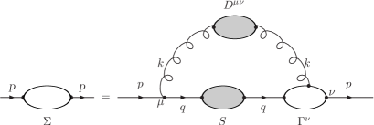
Figure 2: The SD equation (3) for the quark self-energy. The black blobs represent the fully dressed quark and gluon propagators and the white one is the proper quark-gluon vertex.

The first step toward a construction of a manageable system of equations is to ignore the ghost contributions in the quark SD equation. The latter are contained in the full gluon propagator and the full quark-gluon vertex. More specifically, the full quark-gluon vertex should satisfy the Slavnov-Taylor identity

$$i\,k^{\mu}\Gamma_{\mu}(p,q)\left[1+b(k^{2})\right]=$$ (4)

$$=\left[1-B(k,q)\right]S^{-1}(p)-S^{-1}(q)\left[1-B(k,q)\right]\!,$$

where $b(k^{2})$ is the ghost self-energy and $B(k,q)$ is the ghost-quark scattering kernel. Without ghosts, equation (4) becomes identical to the text-book QED Ward identity [6], and the quark-gluon vertex now obeys

$$i\,k^{\mu}\Gamma_{\mu}(p,q)=S^{-1}(p)-S^{-1}(q).$$ (5)

This last Ward identity enforces the equality $Z_{1}=Z_{2}$ between the vertex- and quark-wave-function renormalization constants, exactly as happens in QED. Evidently, in this treatment we are effectively assuming a theory with Abelian-like characteristics, where it is hoped that the form of the effective gluon propagator employed retains some memory of the omitted ghost effects.

The next step is to employ a “gauge technique” inspired Ansatz [7] for the unknown vertex $\Gamma_{\mu}(p,q)$. According to this technique, $\Gamma_{\mu}(p,q)$ is written in terms of $S(p)$ in such way as to satisfy by construction the Ward identity (5). Clearly, this procedure introduces the additional ambiguity of how to fix the transverse part of the vertex, which may lead in higher orders to mishandling of the overlapping divergences, but is expected to be of little consequence in the infrared. In the following analysis we will use for $\Gamma_{\mu}(p,q)$ the simple Ansatz proposed in references [6, 8]

$$i\,\Gamma_{\mu}(p,q)=iA(p^{2})\gamma_{\mu}+$$ (6)

$$+\frac{k_{\mu}}{k^{2}}\Bigl{\{}i\!\left[A(p^{2})-A(q^{2})\right]/{q}+\!\left[B(p^{2})-B(q^{2})\right]\!\Bigr{\}}.$$

Another important consequence of the forced “Abelianization” imposed on the theory establishes finally the required link between the gap equation and the effective QCD charge. In particular, since now $Z_{1}=Z_{2}$, one may define a renormalization-group-invariant quantity, to be denoted by $\alpha(k^{2})$, which is the exact analogue of the QED effective charge, namely

$$g^{2}D_{\mu\nu}(k)=\left\{\delta_{\mu\nu}-\frac{k_{\mu}k_{\nu}}{k^{2}}\right\}\frac{4\pi\alpha(k^{2})}{k^{2}}.$$ (7)

Choosing the Landau gauge leads to the further simplification

$$g^{2}D^{\mu\nu}(k)\Gamma_{\nu}(q,p)=g^{2}D^{\mu\nu}(k)A(q^{2})\gamma_{\nu},$$ (8)

since, in that case, the gluon propagator is completely transverse.

Substituting equations (2) and (8) into the quark gap equation (3), one arrives at the commonly used coupled system for the the quark self-energy in terms of $A(p^{2})$ and $B(p^{2})$ [5, 8]. The last necessary step in order to set up our final quark SD equation is to employ the usual angular approximation, which allows to handle the dependence on the angle appearing in the arguments of the various functions entering into the gap equation. Even though the robustness of this approximation has been occasionally put into doubt (see, for example, [9]), it offers the major advantage of reducing the coupled system to one single equation, since it automatically forces the relation $A(p^{2})=1$. Therefore, we can straightforwardly relate $B(p^{2})$ to the dynamical mass $M(p^{2})$:

$${\mathcal{M}}(x)=\frac{1}{\pi}\left[\frac{\alpha(x)}{x}\int_{0}^{x}\frac{y{\mathcal{M}}(y)}{y+{\mathcal{M}}^{2}(y)}dy+\right.$$

$$\left.+\int_{x}^{\infty}\frac{\alpha(y){\mathcal{M}}(y)}{y+{\mathcal{M}}^{2}(y)}dy\right],$$ (9)

where ${\mathcal{M}}(x)=M(x\Lambda^{2})/\Lambda$, $\,x=p^{2}/\Lambda^{2}$, and $y=q^{2}/\Lambda^{2}$.

Evidently, the invariant charge $\alpha(k^{2})$ lies in the heart of the above equation. Indeed, after the succession of simplifications listed above, it is the sole ingredient which remains to be modeled. It is at this point that the analytic charge $\alpha^{(1)}_{\mbox{\scriptsize an}}(k^{2})$ of (1) will enter into the game, being plugged into equation (Quark gap equation within the analytic approach to QCD) as our model for the QCD effective charge $\alpha(k^{2})$.

Before solving the resulting integral equation numerically, we can infer some qualitative conclusions about the deep infrared behavior of the solutions by differentiating both sides twice with respect to $x$ (see also references [6, 8]), thus converting (Quark gap equation within the analytic approach to QCD) into a differential equation

$${\mathcal{M}}(v)\!\left(\frac{d^{2}}{dv^{2}}+2\frac{d}{dv}\right)\!{\mathcal{M}}(v)=\frac{8}{\beta_{0}v},\;\>v\to-\infty,$$ (10)

where $v=\ln x$. This equation may be solved iteratively; the first iteration, corresponding to the leading infrared behavior of the dynamical mass function ${\mathcal{M}}(x)$, is obtained by omitting the second-order derivative in equation (10). Then, the solution is

$${\mathcal{M}}(x)\simeq\sqrt{\frac{8}{\beta_{0}}\ln|\ln x|},\qquad x\to 0.$$ (11)

The above approximate solution presents a singular behavior in the low-energy region, which can be interpreted as a hint for confinement (see additional discussion in references [4, 8, 10]).

As for the ultraviolet behavior of the solution, the conservation of the axial-vector current eventually leads, for sufficient large momenta, to

$${\mathcal{M}}(x)\simeq\frac{D}{x}(\ln x)^{\lambda-1},\qquad x\to\infty,$$ (12)

where $\lambda=12/(33-2n_{\mbox{\scriptsize f}})$ is the anomalous dimension of the mass, and $D$ is a constant independent of the renormalization point and directly related to the quark condensate (see also review [5] and references therein).

Figure 3: The dimensionless quark dynamical mass ${\mathcal{M}}(x)$, obtained from Eq. (Quark gap equation within the analytic approach to QCD) using the one-loop analytic charge (1) for $n_{\mbox{\scriptsize f}}=4$ active flavors.

The dynamical quark mass function ${\mathcal{M}}(x)$, obtained solving numerically the integral equation (Quark gap equation within the analytic approach to QCD), is presented in Figure 3. Indeed, one can see a soft enhancement of ${\mathcal{M}}(x)$ when $x\to 0$, as forecasted by Eq. (11). In order to restore a physical scale in the dimensionless mass function ${\mathcal{M}}(x)$, one has to relate the obtained solution to a QCD observable. In particular, this can be accomplished by making use of the method developed by Pagels, Stokar [11], and Cornwall [10], which provides the required link between ${\mathcal{M}}(x)$ and the pion decay constant:

$$f_{\pi}^{2}=\!\frac{3\Lambda^{2}}{4\pi^{2}}\!\!\int\limits_{0}^{\infty}\!\left[{\mathcal{M}}(y)\!-\!\frac{y}{2}\frac{d{\mathcal{M}}(y)}{dy}\right]\!\!\frac{y{\mathcal{M}}(y)\,dy}{\left[y+{\mathcal{M}}^{2}(y)\right]^{2}}.$$ (13)

Thus, the scale parameter $\Lambda$ (which is the only adjustable parameter within the approach at hand) can be evaluated by requiring the right-hand side of Eq. (13) to acquire the experimental value of the pion decay constant $f_{\pi}^{2}=(93\,\mbox{MeV})^{2}$. Ultimately, for the case of $n_{\mbox{\scriptsize f}}=4$ active flavors, this results in estimate $\Lambda=880\,$MeV. The higher loop corrections to the analytic running coupling $\alpha_{\mbox{\scriptsize an}}(k^{2})$ [3] do not alter qualitatively the picture obtained. Specifically, the confining behavior of the dynamical mass function ${\mathcal{M}}(x)$ persists, but the infrared singularity displayed is weaker than that of Eq. (11). In turn, this further elevates the estimate of the scale parameter $\Lambda$.

The conclusion that we draw from the above analysis is that the analytic invariant charge developed in Ref. [3] and the SD equations may coexist in a complementary and qualitatively consistent picture, and that the obtained value for the only free parameter turns out to be in the right ballpark.

References

- [1] D.V. Shirkov and I.L. Solovtsov, Phys. Rev. Lett. 79, 1209 (1997); D.V. Shirkov, Eur. Phys. J. C 22, 331 (2001).
- [2] K.A. Milton and I.L. Solovtsov, Phys. Rev. D 55, 5295 (1997); 59, 107701 (1999); A.P. Bakulev, S.V. Mikhailov, and N.G. Stefanis, hep-ph/0506311.
- [3] A.V. Nesterenko, Phys. Rev. D 62, 094028 (2000); 64, 116009 (2001); Int. J. Mod. Phys. A 18, 5475 (2003); Nucl. Phys. B (Proc. Suppl.) 133, 59 (2004).
- [4] A.C. Aguilar, A.V. Nesterenko, and J. Papavassiliou, J. Phys. G 31, 997 (2005).
- [5] C.D. Roberts and A.G. Williams, Prog. Part. Nucl. Phys. 33, 477 (1994).
- [6] D. Atkinson and P.W. Johnson, Phys. Rev. D 37, 2290 (1988); 37, 2296 (1988); D. Atkinson, P.W. Johnson, and K. Stam, ibid. D 37, 2996 (1988).
- [7] A. Salam, Phys. Rev. 130, 1287 (1963); A. Salam and R. Delbourgo, ibid. 135, 1398 (1964); R. Delbourgo and P. West, J. Phys. A 10, 1049 (1977); Phys. Lett. B 72, 96 (1977); R. Delbourgo and R.B. Zhang, J. Phys. A 17, 3593 (1984).
- [8] G. Krein, P. Tang, and A.G. Williams, Phys. Lett. B 215, 145 (1988).
- [9] J. Papavassiliou and J.M. Cornwall, Phys. Rev. D 44, 1285 (1991).
- [10] J.M. Cornwall, Phys. Rev. D 22, 1452 (1980).
- [11] H. Pagels and S. Stokar, Phys. Rev. D 20, 2947 (1979).