Introduction

In this talk I have discussed two issues regarding pentaquarks in chiral soliton models. First I have reviewed the relation between exotic five–quark states and radial excitations. In particular I have explained that the wave–functions of the crypto–exotic partners of the pentaquarks have significant admixture of radial excitations of the ordinary baryons and that this may have significant impact on transition magnetic moments. I have extensively described that issue before [1] and will abstain from repeating it in these proceedings. Rather, I will focus on the second topic of my talk which deals with potential differences between the bound state and rigid rotator approaches (BSA and RRA, respectively) to generate baryon states with non–zero strangeness from the classical soliton; two seemingly different treatments of the same model. It has previously been argued that the prediction of pentaquarks, i.e. exotic baryons with strangeness $S=+1$, would be a mere artifact of the RRA [2]. A major result of the investigation presented in this talk is that pentaquark states do indeed emerge in both approaches. This comparison furthermore shows how to unambiguously compute the width of pentaquarks. That computation of the width differs substantially from previous approaches based on assuming pertinent transition operators for $\Theta^{+}\to KN$ [3, 4]. Details of these studies and an exhaustive list of relevant references are contained in the recent paper [5] in collaboration with Hans Walliser.

The qualitative results, on which I focus, are model independent while quantitative results may be quite sensitive to the model parameters and/or the actual form of the chiral Lagrangian. For simplicity, our calculations in ref. [5] have been performed in the Skyrme model augmented by the Wess–Zumino and the simplest flavor symmetry breaking terms. The latter parameterizes the kaon–pion mass difference.

Chiral soliton calculations are organized in powers of $N_{C}$, the number of colors and hidden expansion parameter of QCD. The leading contribution is the classical soliton energy, $E_{\rm cl}={\cal O}(N_{C})$. The reported calculation is complete to ${\cal O}(N_{C}^{0})$, identifies the resonance contribution in kaon–nucleon scattering and provides insight in $1/N_{C}$ corrections.

Small amplitude vs. collective coordinate quantization

I start with phrasing the problem and briefly review the two popular approaches to generate baryon states with strangeness $S=\pm 1$ from a soliton configuration. Chiral soliton models are in general functionals of the chiral field, $U$, the non–linear realization of the pseudoscalar fields. Starting point in these considerations is the classical soliton, i.e. the hedgehog embedded in the isospin subgroup of flavor $SU(3)$,

$$U_{0}(\vec{x\,})={\rm exp}\left[i\vec{\tau\,}\cdot\hat{x}F(r)\right]\,,\quad r=|\vec{x\,}|$$ (1)

parameterized by the three Pauli matrices $\tau_{i}$. The essential issue, however, is the treatment of the strange degrees of freedom, the kaons.

The ansatz for small amplitude quantization of kaon modes, known as BSA, reads

$$U(\vec{x\,},t)=A_{2}(t)\sqrt{U_{0}(\vec{x\,})}\,\,{\rm exp}\left[\frac{i}{f_{\pi}}\sum_{\alpha=4}^{7}\lambda_{\alpha}\eta_{\alpha}(\vec{x\,},t)\right]\sqrt{U_{0}(\vec{x\,})}\,A_{2}^{\dagger}(t)\,,$$ (2)

where $\lambda_{\alpha}$ are Gell–Mann matrices of $SU(3)$. The small amplitude fluctuations $\eta_{\alpha}$ are treated in harmonic approximation. The pion decay constant, $f_{\pi}$ is ${\cal O}(\sqrt{N_{C}})$. Hence this harmonic expansion is complete at ${\cal O}(N_{C}^{0})$. Subleading contributions may be substantial but they are not under control in the BSA. The dynamical treatment of the collective coordinates, $A_{2}\in SU(2)$ for the spin–isospin orientation of the soliton adds some of them. Quantization of both $\eta_{\alpha}$ and $A_{2}$ results in the mass formula

$$M_{S}=E_{\rm cl}+\omega_{S}+\frac{1}{2\Theta_{\pi}}\left[c_{S}J\left(J+1\right)+\left(1-c_{S}\right)I\left(I+1\right)\right]+{\cal O}\left(\eta^{4}\right)\,.$$ (3)

for strangeness $S=\pm 1$ baryons. Here $J$ and $I$ are the spin and isospin quantum numbers of the considered baryon, respectively. The parameters in eq. (3) can be approximated as functionals of the chiral angle, $F(r)$ and are conveniently described by defining $\omega_{0}=\frac{N_{C}}{4\Theta_{K}}$,

$$\omega_{\pm}=\frac{1}{2}\left[\sqrt{\omega_{0}^{2}+\frac{3\Gamma}{2\Theta_{K}}}\pm\omega_{0}\right]\quad{\rm and}\quad c_{\pm}=1-\frac{4\Theta_{\pi}\omega_{\pm}}{8\Theta_{K}\omega_{\pm}\mp N_{C}}\,.$$ (4)

The difference between $\omega_{+}$ and $\omega_{-}$ originates from the Wess–Zumino term. Explicit expressions for the moments of inertia $\Theta_{\pi}$ (rotation in coordinate space) and $\Theta_{K}$ (rotations in $SU(3)$ flavor space) as well as the symmetry breaking parameter $\Gamma$ (proportional to $m_{K}^{2}-m_{\pi}^{2}$) may be traced from the literature [5]. They are all ${\cal O}(N_{C})$.

The second approach treats the kaon modes purely as collective excitations of the classical soliton, eq. (1). These collective modes are maintained to all orders and quantized canonically. The ansatz for this so–called rigid rotator approach (RRA) reads

$$U(\vec{x\,},t)=A_{3}(t)U_{0}(\vec{x\,})\,A_{3}^{\dagger}(t)\quad{\rm with}\quad A_{3}(t)\in SU(3)\,.$$ (5)

This parameterization describes only a limited number of soliton excitations, those that arise as a rigid rotation of the classical soliton. Though generating contributions of ${\cal O}(N_{C}^{0})$ to baryon masses it is not complete at this order, e.g. S–wave excitations are not accessible. However, since the rigid rotations are treated to any order, they control significant subleading effects on the low–lying P–wave baryons. From the ansatz, eq. (5) the Hamiltonian for the collective coordinates is straightforwardly derived. The corresponding baryon spectrum is the solution to the eigenvalue problem ($D_{ab}=\frac{1}{2}{\rm tr}[A\lambda_{a}A^{\dagger}\lambda_{b}]$)

$$\left\{\left(\frac{1}{2\Theta_{\pi}}-\frac{1}{2\Theta_{K}}\right)J(J+1)+\sum_{a=1}^{7}\frac{R_{a}^{2}}{2\Theta_{K}}+\frac{\Gamma}{2}\left(1-D_{88}\right)\right\}\Psi={\cal E}\Psi\,,\quad R_{8}\Psi=\frac{N_{C}}{2\sqrt{3}}\Psi\,,$$ (6)

in each spin–isospin channel. The $R_{a}$ denote the (intrinsic) $SU(3)$ generators conjugate to the collective rotations $A_{3}\in SU(3)$. This eigenvalue problem is (numerically) exactly solved for arbitrary (odd) $N_{C}$ and symmetry breaking $\Gamma$ by generalizing the techniques of ref. [6]. Then the eigenvalues ${\cal E}$ determine the baryon spectrum. In the flavor symmetric case the eigenstates are members of $SU(3)$ representations. For $N_{C}=3$ those are the octet and the decuplet for the low–lying $J={\textstyle\frac{1}{2}}$ and $J={\textstyle\frac{3}{2}}$ baryons, respectively. Also states in the anti–decuplet, $\mathbf{\overline{10}}$ are low–lying. Probably the lowest mass state in the $\mathbf{\overline{10}}$ is the $\Theta^{+}$ pentaquark. For arbitrary $N_{C}$ the condition on $R_{8}$ alters the allowed $SU(3)$ representations and the inclusion of flavor symmetry breaking leads to mixing of states from different representations. These effects are incorporated in the exact numerical solution. In figs. 1 and 2 I compare the spectra for the low–lying P–wave baryons obtained from eqs. (3) and (6) as functions of $N_{C}$.

             

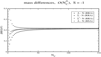
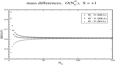
Fig. 1: Mass differences at ${\cal O}(N_{C}^{0})$ computed within the bound state and rigid rotator approaches (BSA and RRA, respectively) in the Skyrme model as functions of $N_{C}$. In the RRA they are the corresponding differences of the eigenvalues in eq. (6) while in the BSA they are extracted from eq. (3). Left panel $\Delta S=-1$; right panel $\Delta S=+1$.

             

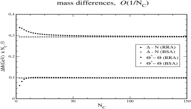
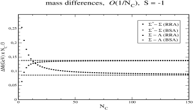
Fig. 2: Mass differences at ${\cal O}(1/N_{C})$ computed in the Skyrme model as functions of $N_{C}$. Left panel: baryons with strangeness $S=0,1$; right panel $S=-1$. See also caption of fig. 1.

Obviously the two approaches yield identical results as $N_{C}\to\infty$, as they should. This is the case for the ordinary hyperons and the pentaquarks. Fig. 2 also shows that even with flavor symmetry breaking included, the $\Delta$–nucleon mass difference is ${\cal O}(1/N_{C})$ in contrast to what is stated in ref. [7].

Constrained fluctuations and $\mathbf{\Theta^{+}}$ width

The above observed identity between BSA and RRA in the large $N_{C}$ limit has a caveat. Though $\omega_{-}<m_{K}$ corresponds to a true bound state, $\omega_{+}$ is a continuum state. Thus, a pronounced resonance structure is expected in the corresponding phase shift. However, that is not the case, as indicated in the left panel of fig. 3. The computed phase shift hardly reaches $\pi/2$ rather then quickly passing through this value. This has been used to argue that pentaquarks are a mere artifact of the RRA [2]. However, the ultimate comparison requires to generalize the RRA to the rotation–vibration approach (RVA)

$$U(\vec{x\,},t)=A_{3}(t)\sqrt{U_{0}(\vec{x\,})}\,{\rm exp}\left[\frac{i}{f_{\pi}}\sum_{\alpha=4}^{7}\lambda_{\alpha}\widetilde{\eta}_{\alpha}(\vec{x\,},t)\right]\sqrt{U_{0}(\vec{x\,})}\,A_{3}(t)^{\dagger}\,.$$ (7)

Modes that correspond to the collective rotations must be excluded from the fluctuations $\widetilde{\eta}$, i.e. the fluctuations must be orthogonal to the zero–mode $z(r)\sim{\rm sin}\left(\frac{F(r)}{2}\right)$. Imposing the corresponding constraints for these fluctuations (and their conjugate momenta) yields integro–differential equations listed in ref. [5]. For the moment let’s omit the coupling between $\widetilde{\eta}$ and the collective soliton excitations (eigenstates of eq. (6), including pentaquarks). This truncation defines the background wave–function $\overline{\eta}$ (also orthogonal to the zero mode). Treating $\overline{\eta}$ as an harmonic fluctuation provides the background phase shift shown as the blue curve in the right panel of fig. 3. Remarkably, the difference between the phase shifts of $\overline{\eta}$ and $\eta$ exhibits a clear resonance structure. It is the resonance phase shift to be associated with the $\Theta^{+}$ pentaquark in the limit $N_{C}\to\infty$.

There is an even more convincing computation of this resonance phase shift. In contrast to the parameterization, eq. (2) the ansatz, eq. (7) yields an interaction Hamiltonian that is linear in the fluctuations, generating Yukawa couplings between the collective soliton excitations and the fluctuations $\widetilde{\eta}$. In ref. [5] we have derived this Hamiltonian keeping all contributions that survive as $N_{C}\to\infty$. The corresponding Yukawa exchanges extend the integro–differential equations for $\overline{\eta}$ by a separable potential $V_{Y}$, therewith providing the equations of motion for $\widetilde{\eta}$ [5]. The equation of motion for $\widetilde{\eta}$ is solved by $\widetilde{\eta}=\eta-az$ with $a=\langle z|\eta\rangle$ for $N_{C}\to\infty$ [5], where $\eta$ is the unconstrained small amplitude fluctuation of the BSA, eq. (2). The phase shifts extracted from $\eta$ and $\widetilde{\eta}$ are identical because $z(r)$ is localized in space.

             

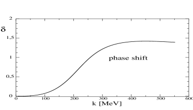
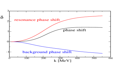
Fig. 3: Phase shift computed in the BSA (left panel) and resonance phase shift after removal of the background contribution in the RVA (right panel). Note the different scales.

Thus the BSA and RVA yield the same spectrum and are indeed equivalent in the large $N_{C}$ limit. But, the RVA provides a distinction between resonance and background contributions to the scattering amplitude. Applying the $R$–matrix formalism on top of the constrained fluctuations $\overline{\eta}$ shows that $V_{Y}$ exactly contributes the resonance phase shift shown in fig. 3 when the Yukawa coupling is computed for $N_{C}\to\infty$. This identifies the exchange of a state predicted in the RRA which thus is no artifact. In contrast, pentaquarks are also predicted by the BSA; just well hidden. However, collective coordinates are mandatory to obtain finite $N_{C}$ corrections to the BSA for the properties of $\Theta^{+}$. Though not all ${\cal O}(1/N_{C})$ operators were included in ref. [5], subleading effects have turned out to be substantial. For example, in the case $m_{K}=m_{\pi}$ the mass difference with respect to the nucleon increases by a factor two from $\omega_{0}$ to $(N_{C}+3)/4\Theta_{K}$ for $N_{C}=3$. In the realistic case with $m_{K}\neq m_{\pi}$ this mass difference is obtained from solving the eigenvalue problem, eq. (6). Furthermore, the resonance (extracted from the comparison between $\widetilde{\eta}$ and $\overline{\eta}$) becomes sharper as $N_{C}<\infty$ [5].

The separable potential $V_{Y}$ also provides the general expression for the width as a function of the kaon energy $\omega_{k}=\sqrt{k^{2}+m_{K}^{2}}$ from the $R$–matrix formalism [5]

$$\Gamma(\omega_{k})=2k\omega_{0}\left|X_{\Theta}\int_{0}^{\infty}r^{2}dr\,z(r)2\lambda(r)\overline{\eta}_{\omega_{k}}(r)+\frac{Y_{\Theta}}{\omega_{0}}\left(m_{K}^{2}-m_{\pi}^{2}\right)\int_{0}^{\infty}r^{2}dr\,z(r)\overline{\eta}_{\omega_{k}}(r)\right|^{2}\,.$$ (8)

Here $\overline{\eta}_{\omega_{k}}(r)$ is the P–wave projection of the background wave–function $\overline{\eta}$ for a prescribed energy $\omega_{k}$. Furthermore $\lambda(r)$ is a radial function that stems from the Wess–Zumino term. The matrix elements of the collective coordinate operators that enter in eq. (8) ($D_{\pm a}=D_{4a}\pm iD_{5a}$)

$$X_{\Theta}:=\sqrt{\frac{32}{N_{C}}}\langle\Theta^{+}|\sum_{\alpha,\beta=4}^{7}d_{3\alpha\beta}D_{+\alpha}R_{\beta}|n\rangle\,,\qquad Y_{\Theta}:=\sqrt{\frac{8N_{C}}{3}}\langle\Theta^{+}|\sum_{\alpha,\beta=4}^{7}d_{3\alpha\beta}D_{+\alpha}D_{8\beta}|n\rangle$$ (9)

approach unity as $N_{C}\to\infty$ in the flavor symmetric case. In general they are computed from the eigenstates of the collective coordinate Hamiltonian, eq. (6). The resulting width is shown for $N_{C}=3$ in fig. 4 for the flavor symmetric case and the physical kaon–pion mass difference.

Fig. 4: Model prediction for the decay width, $\Gamma(\omega)$ of $\Theta^{+}$ for $N_{C}=3$ as function of the kaon momentum $k=\sqrt{\omega^{2}-m_{K}^{2}}$, cf. eq. (8). Top: $m_{K}=m_{\pi}$, bottom: $m_{K}\neq m_{\pi}$.

As function of momentum, there are only minor differences between these two cases. Assuming the observed resonance to be the (disputed [8]) $\Theta^{+}(1540)$ a width of roughly $40{\rm MeV}$ is read off from fig. 4 [5]. It should be kept in mind that the general results on the treatment of strange degrees of freedom are model independent but the numerical results for the masses and the widths of pentaquarks are not.

Conclusion

In this talk I have presented a thorough comparison [5] between the bound state (BSA) and rigid rotator approaches (RRA) to chiral soliton models in flavor $SU(3)$. For definiteness I have only considered the simplest version of the Skyrme model augmented by the Wess–Zumino and symmetry breaking terms. However, this analysis merely concerns the treatment of kaon degrees of freedom. Therefore the qualitative results are valid for any chiral soliton model.

A sensible comparison with the BSA requires the consideration of harmonic oscillations in the RRA as well. They can indeed be incorporated via the rotation–vibration approach (RVA), however constraints must be implemented to ensure that the introduction of such fluctuations does not double–count any degrees of freedom. The RVA clearly shows that the prediction of pentaquarks is not an artifact of the RRA, pentaquarks are genuine within chiral soliton models. Only within the RVA chiral soliton models generate interactions for hadronic decays. Technically the derivation of this Hamiltonian is quite involved, however, the result is as simple as convincing: In the limit $N_{C}\to\infty$, in which the BSA is undoubtedly correct, the RVA and BSA yield identical results for the baryon spectrum and the kaon–nucleon $S$-matrix. This identity also holds when flavor symmetry breaking is included. This is very encouraging as it demonstrates that collective coordinate quantization may be successfully applied regardless of whether or not the respective modes are zero–modes. Though the large $N_{C}$ limit is helpful for testing the results of the RVA, taking only leading terms in the respective matrix elements is not trustworthy.

In the flavor symmetric case the interaction Hamiltonian contains only a single structure ($X_{\Theta}$) of $SU(3)$ matrix elements for the $\Theta^{+}\to KN$ transition. Any additional $SU(3)$ structure only enters via flavor symmetry breaking. This proves earlier approaches [3, 4] incorrect that adopted any possible structure that would contribute in the large $N_{C}$ limit and fitted coefficients from a variety of hadronic decays under the assumption of $SU(3)$ relations. That treatment yielded a potentially small $\Theta^{+}$ width from cancellations between different such structures even in the flavor symmetric case. The study presented in this talk thus clearly shows that it is not worthwhile to bother about the obvious arithmetic error in ref. [3] that was discovered earlier [1, 9] because the conceptual deficiencies in such width calculations are more severe. Assuming $SU(3)$ relations among hadronic decays is not a valid procedure in chiral soliton models. The embedding of the classical soliton breaks $SU(3)$ and thus yields different structures for different hadronic transitions. Especially strangeness conserving and changing processes are not related to each other in chiral soliton model treatments.

Even in case pentaquarks turn out not to be what recent experiments have indicated, they have definitely been very beneficial in combining the bound state and rigid rotator approaches and solving the Yukawa problem in the kaon sector; both long standing puzzles in chiral soliton models.

Acknowledgments

I am grateful to the organizers for this pleasant workshop. I am very appreciative to Hans Walliser for the fruitful collaboration without which this presentation would not have been possible.

References

- [1] H. Weigel, Eur. Phys. J. A 2 (1998) 391; AIP Conf. Proc. 549 (2002) 271; Eur. Phys. J. A21 (2004) 133; arXiv:hep-ph/0410066.
-
[2]
N. Itzhaki, I. R. Klebanov, P. Ouyang and L. Rastelli,
Nucl. Phys. B684 (2004) 264.
T. D. Cohen, Phys. Lett. B581 (2004) 175; arXiv:hep-ph/0312191.
A. Cherman, T. D. Cohen, T. R. Dulaney and E. M. Lynch, arXiv:hep-ph/0509129. - [3] D. Diakonov, V. Petrov, M. Polyakov, Z. Phys. A359 (1997) 305
-
[4]
J. R. Ellis, M. Karliner, M. Praszałowicz,
JHEP 05 (2004) 002.
M. Praszałowicz, Acta Phys. Polon. B35 (2004) 1625.
M. Praszałowicz and K. Goeke, Acta Phys. Polon. B36 (2005) 2255, [hep-ph/0506041]. - [5] H. Walliser, H. Weigel, arXiv:hep-ph/0510055.
- [6] H. Yabu and K. Ando, Nucl. Phys. B301 (1988) 601.
- [7] M. Praszałowicz, Phys. Lett. B583 (2004) 96.
-
[8]
K. Hicks,
J. Phys. Conf. Ser. 9 (2005) 183
S. Kabana, AIP Conf. Proc. 756 (2005) 195. - [9] R. L. Jaffe, Eur. Phys. J. C 35 (2004) 221.