FTPI-MINN-05/44

UMN-TH-2417/05

October 13/05

$k$ Strings from Various Perspectives:

QCD, Lattices, String Theory and Toy Models 

M. Shifman

William I. Fine Theoretical Physics Institute, University of Minnesota, Minneapolis, MN 55455, USA

I review the status of the issue of the $k$-string tension in Yang–Mills theory. After a summary of known facts I discuss a weakly coupled four-dimensional Yang–Mills theory that supports non-Abelian strings and can, in certain aspects, serve as a toy model for QCD strings. In the second part of the talk I present original results obtained in a two-dimensional toy model which provides some evidence for the sine formula.

1 Preamble

Valya Zakharov was the first to introduce me to QCD, even before QCD was officially born. In the summer of 1972 he was sent, as the ITEP Ambassador, to the Rochester conference which took place at Fermilab that year. After his return, he told us of his impressions.

Apparently, Gell-Mann’s talk produced the strongest impression on Valya since he kept saying that Gell-Mann had been preaching octet gluons as mediators of the inter-quark force, and we ought to do something. I was in the very beginning of my PhD work at that time, and knew very little as to how to orient myself in the sea of literature, and whom to trust. Valya repeated, more than once, that Gell-Mann had a direct line to god — Gell-Mann’s revelations ought to be taken seriously.

It would be fair to say that Valya’s persistence and foresight shaped my career to a large extent. It is gratifying to note that now, 33 years later, he continues a noble mission of analytic thinking, deep insight and promotion of innovative ideas in the lattice QCD community. Thank you, Valya, and Happy Birthday …

Part I: Review

2 Introduction

For this talk I chose a topic seemingly fitting well the scope of Zakharov’s interests which in the recent years revolve around various mechanisms of color confinement in Yang–Mills (YM) theories. The issue I want to address is the $k$-string tension. Significant effort has been invested recently in QCD and YM theories at large in the studies of flux tubes induced by color sources in higher representations of SU($N$), mostly in connection — but not exclusively — with high-precision lattice calculations (for a review see [1] and references therein; see also Sect. 9). If a source has $k$ fundamental color indices ($N$-ality $k$), the flux tube it generates is referred to as the $k$-string. The question of $k$ and $N$ dependence of the $k$-string tension is one of the central questions of color-confining dynamics.

For many years the prevailing hypothesis was that of the so-called Casimir scaling, the genesis of which can be seemingly traced back to various models based on one-gluon exchange, popular in the 1970’s and 80’s, as well as to the strong-coupling lattice expansions. Surprisingly, only recently it was realized [2, 3] that the Casimir scaling is in direct contradiction with the $1/N$ expansion in YM theory.

Meanwhile, an alternative construction emerged which does have an appropriate $1/N$ expansion. It goes under the name of the sine formula for the $k$-string tension. Originally it was suggested by Douglas and Shenker [4] in connection with ${\cal N}=2$ super-Yang–Mills model. Arguments in favor of this formula were obtained in MQCD and supersymmetric theories (for a detailed discussion and a representative list of references see [2, 3]).

In spite of the abundance of arguments, and the correct $1/N$ behavior inherent to the sine formula, it has never been proven, and the issue of its relevance to QCD remains open. This talk consists of two parts. Part I is designed as a brief review of general ideas regarding QCD $k$-strings, with the emphasis on developments after 2003. For a review of the pre-2003 situation the reader is referred to [3]. Part II is original. It presents a toy model in which the exact sine formula for an analog of the $k$-string tension emerges in a natural way. This toy model is two-dimensional but it is closely (in fact, “genetically”) related to a four-dimensional weakly coupled gauge model which has been recently developed, see [5, 6], and references therein, and Sect. 10. Its remarkable feature is that it supports non-Abelian strings, pretty close relatives of QCD strings, the main subject of our analysis.

3 Strings/flux tubes in known phenomena

A physical phenomenon where flux tubes with well-studied properties are proven to play a crucial role is known from 1930s and to theorists from 1950s. In 1957 Abrikosov published the paper [7] entitled On the Magnetic Properties of Superconductors of the Second Type which deals with penetration of magnetic fields in bulk superconductors. Magnetic flux is conserved. If one places a large bulk superconductor between two poles of a magnet, the magnetic field must go through, but it cannot go through without destroying superconductivity. Treating the Cooper pair condensation in the framework of the Ginzburg–Landau theory, Abrikosov found vortex-type solutions describing magnetic fields squeezed into thin tubes carrying the total magnetic flux which is quantized. The corresponding physical phenomenon is called the Meissner effect. Superconductivity is destroyed in the core of the tubes. The energy of such configurations is $\sigma L$ where $\sigma$ is the string tension and $L$ is the size of the bulk superconductor pierced by the flux tube. The energy scales linearly with the size. The flux tubes end on the poles of the magnet or, if magnetic monopole existed, they could end on the magnetic monopoles.

The Abrikosov flux tubes are currently known as Abelian or U(1) flux tubes. They emerge in the Abelian Higgs model (see [8]) due to the fact that $\pi_{1}({\rm U}(1))$ is non-trivial. The gauge U(1) symmetry is spontaneously broken in the vacuum by a condensate of a charged scalar field $\phi$, the Higgs field, which can be thought of as representing the Cooper pair density. The string configuration, with a winding phase of the scalar field $\phi$, is topologically stable. At large distances from string’s core $|\phi|$ coincides with its vacuum value, while inside the core $\phi\to 0$. Thus, superconductivity is destroyed in string’s core. The magnetic flux transmitted through the Abrikosov–Nielsen–Olesen (ANO) flux tube can be arbitrary integer number (in appropriate units).

4 Color confinement: dual Meissner effect hypothesis

Magnetic charges attached to the endpoints of the Abrikosov string are confined: taking them apart would require infinite energy. In QCD we want chromoelectric charges, rather than chromomagnetic ones, to be attached to the endpoints of the chromoelectric flux tubes and thus confined. Chromomagnetic charges must condense. In the 1970s ’t Hooft [9] and Mandelstam [10] put forward the hypothesis of a dual Meissner effect to explain color confinement in non-Abelian gauge theories. Dual means that we take the Abrikosov theory and replace everything electric by magnetic and vice versa.

The ’t Hooft-Mandelstam hypothesis was formulated at a qualitative level. Since then people kept trying to find a quantitative framework in which one could demonstrate the occurrence of the dual Meissner effect in a controllable approximation: formation of chromoelectric flux tubes with properties compatible with general ideas and existing data on color confinement. This task proved to be extremely difficult.

A breakthrough achievement was the Seiberg–Witten solution [11] of ${\cal N}=2$ supersymmetric Yang–Mills theory. They found massless monopoles at a certain point in the moduli space and, adding a small $({\cal N}=2)$-breaking deformation, demonstrated that they condense creating strings carrying a chromoelectric flux. This was the first quantitative implementation of the ’t Hooft–Mandelstam hypothesis, 16 years after its inception! Needless to say, the Seiberg–Witten result was met with great enthusiasm in the community.

A more careful examination showed, however, that details of the Seiberg–Witten confinement were quite different from those we expect in QCD-like theories. Indeed, a crucial aspect of Ref. [11] is that the SU($N$) gauge symmetry is first broken, at a high scale, down to U(1)^N-1, which is then completely broken, at a much lower scale where monopoles condense. Correspondingly, the Seiberg-Witten model strings are, in fact, the Abelian strings [7, 8] of the Abrikosov–Nielsen–Olesen type. This leads to an “Abelian” confinement whose structure does not resemble at all that of QCD. In particular, the “hadronic” spectrum is much richer than that in QCD [4, 12]. For a review see [13].

Thus, the task of constructing and studying non-Abelian strings in QCD and QCD-like theories still stands. I will summarize recent (modest) progress [14, 15, 16, 5, 6, 17, 18, 19] at the end of Part I. However, to begin with, it is instructive to discuss what we know of QCD strings from $1/N$, lattices, and other ideas.

5 QCD strings

The simplest QCD string is the flux tube that connects heavy (probe) color sources in the fundamental representation. It is referred to as the fundamental string. The fundamental string tension is of the order of $\Lambda^{2}$ where $\Lambda$ is the dynamical scale parameter. Its transverse size is of the order of $\Lambda^{-1}$. Both parameters are independent of the number of colors, and, besides $\Lambda$, can contain only numerical factors. In what follows I assume the gauge group to be SU($N$), with $N$, the number of colors, being a free parameter and $g^{2}N$ fixed.

The flux tubes attached to color sources in higher representations of SU($N$) are known as $k$-strings, where $k$ denotes the $N$-ality of the color representation under consideration. The $N$-ality of the representation with $\ell$ upper and $m$ lower indices (i.e. $\ell$ fundamental and $m$ anti-fundamental) is defined as

$$k=|\ell-m|\,.$$ (5.1)

Figure 1 displays the fundamental string and 2-string. Since $N$ fundamental quarks can form a color-singlet object (baryon), $N$-ality is defined mod $N$.

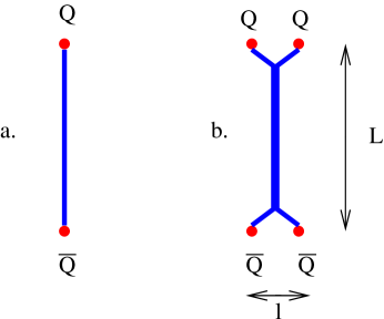
Figure 1: A flux tube for $k$-strings: (a) the fundamental tube; (b) the 2-string tube.

$N$ fundamental strings collected together, as in Fig. 1b, will pass into a no-string state. This feature of non-Abelian strings critically distinguishes them from the ANO strings. For the same reason, if, say, $N$ is odd, $k$-strings with $k=\frac{1}{2}(N\pm 1)$ must be identical. The same is true for $k=\frac{1}{2}(N\pm 2)$ if $N$ is even.

The $k$-string tension cannot depend on particular representation of the probe color source, but only on its $N$-ality. Indeed, the particular Young tableau of the representation plays no role, since all representations with the given $N$-ality can be converted into each other through emission of an appropriate number of soft gluons. For instance, the adjoint representation has vanishing $N$-ality; the color source in the adjoint can be completely screened by gluons, and the flux tube between the adjoint color sources should not exist. The symmetric two-index representation $Q^{\{ij\}}$ can be transformed into antisymmetric $Q^{[ij]}$ plus a gluon, $Q^{\{ij\}}\to Q^{[ik]}+G_{k}^{j}$, and so on.

The above statement seemingly contradicts the abundant lattice literature on the adjoint strings, measurements of distinct string tensions for symmetric and anti-symmetric representations of one and the same $N$-ality, and so on. Does it?

It turns out that at large $N$ some “wrong” strings are quasi-stable. Being created, they must relax to bona fide $k$-strings (i.e. those corresponding to sources with $k$ indices in fully antisymmetric representation), but the relaxation time is exponentially large. Surprisingly, the question how fast they relax has never been solved previously. I will present a sample estimate for the two-index symmetric representation in Sect. 7. In this case to measure the bona fide $2$-string tension one should deal with Wilson contours whose area is much larger than exp$(\gamma N^{2})$, where $\gamma$ is a numerical constant.

6 Casimir vs. sine formula

If $\sigma_{f}$ is the tension of the fundamental string, the Casimir formula reads

$$\sigma_{k}=\frac{C_{R}}{C_{\rm fund}}\,\sigma_{\rm f}$$ (6.1)

where $C_{R}$ is the quadratic Casimir coefficient for representation $R$ defined as

$$T^{a}T^{a}=C_{R}\,I_{R}$$

(here $I$ is the unit matrix in the representation $R$, while $T^{a}$’s stand for the SU$(N)$ generators in the same representation). For antisymmetric $k$-index representation

$$\sigma_{k}=k\left(1-\frac{k-1}{N-1}\right)\,\sigma_{\rm f}\,.$$ (6.2)

The large-$N$ expansion of the Casimir formula is

$$\sigma_{k}=k\left(1-\frac{k}{N}+O(N^{-2})\right)\,\sigma_{\rm f}\,.$$ (6.3)

The expansion runs in even and odd powers of $1/N$.

Now, let us compare it with the sine law for the $k$-string tension which reads

$$\sigma_{k}=\left(\sin\frac{\pi}{N}\right)^{-1}\sigma_{\rm f}\,\sin\left(\frac{\pi\,k}{N}\right)\,.$$ (6.4)

At large $N$ the sine formula can be expanded as follows:

$$\sigma_{k}=k\left(1-\frac{\pi^{2}}{6N^{2}}\,(k^{2}-1)+O(N^{-4})\right)\,\sigma_{\rm f}\,.$$ (6.5)

The difference which immediately becomes obvious is that in the sine formula the large-$N$ expansion runs in even powers of $1/N$ while in the Casimir formula all powers of $1/N$ are involved.

Let us ask ourselves what should one expect in Yang–Mills theory. Assume that we start from two distant fundamental strings, each attached to a (infinitely heavy) probe quark at the top and a probe antiquark at the bottom, as in Fig. 1. The distance between the probe quark and antiquark is $L\to\infty$. the distance between two $Q$’s is $\ell$, and so is the distance between two $\bar{Q}$’s. No dynamical quarks are present in our theory. Then we let two $Q$’s adiabatically approach each other, keeping the strings parallel, and eventually make the distance $\ell$ between them less than $\Lambda^{-1}$.

At $N=\infty$ the energy of this configuration is $2\sigma_{\rm f}L+\,L$-independent part which is irrelevant for our purposes. In this limit the two strings do not interact. At finite $N$ interaction switches on. The spatial extent of interaction is $\sim\Lambda^{-1}$. If we consider parts of strings in the central domain, far away from the endpoints, the interaction has no knowledge of quarks whatsoever (Fig. 2a). In fact, in supersymmetric gluodynamics one could eliminate probe quarks at all, putting the endpoints of the strings under consideration on two distant parallel domain walls. The large-$N$ structure of the interaction is the same as in pure Yang–Mills. Hence, the $1/N$ expansion runs in even powers [3].

One can arrive at the same conclusion from the string theory side too [3], see Fig. 2b. Time axis is in the horizontal direction, we have two parallel fundamental string worldsheets, and their interaction is due to the closed string exchange (annulus diagram). It is quite obvious that this contribution is proportional to $g_{\rm st}^{2}$ where $g_{\rm st}$ is the string coupling constant. Since $g_{\rm st}\sim 1/N$ we see again that the string interaction starts from $1/N^{2}$ and contains only even powers of $1/N$.

One can argue on general grounds that at distances $\mathrel{\hbox to0.0pt{\lower 4.0pt\hbox{\hskip 1.0pt$\sim$}\hss}\raise 1.0pt\hbox{$>$}}\Lambda^{-1}$ the fundamental strings attract each other [3], while at short distances there is a repulsion, so that composite $k$-strings do develop. The Casimir scaling as an exact formula for the $k$-string tension is excluded. The sine formula does have an appropriate $1/N$ expansion, but this is certainly no proof.

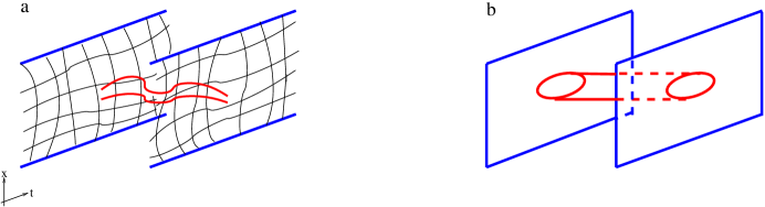
Figure 2: The interaction of two “fundamental” strings: (a) Field-theory picture — (two)gluon exchange; (b) String-theory picture — exchange of a closed string between two worldsheets.

Needless to say, getting a clear-cut understanding of the status of the sine formula in large-$N$ QCD is highly desirable. Unfortunately, there was no dramatic progress in this issue since 2003. Still, two remarks are in order.

The first remark concerns the derivation of the $k$-string tension via supergravity. For the Maldacena–Nuñez background [20] the sine formula was found to be exact [21]. At the same time, for the Klebanov–Strassler background [22] the sine formula proved to be an excellent approximation, valid to a few percent accuracy, but not exact. (Of course, the even power $1/N$ expansion applies in both cases.) Recently Butti et al. realized [23] that the Klebanov–Strassler solution is a limiting case of an entire branch of solutions which goes under the name of a “baryonic branch.” By varying the string coupling and some other parameters one can smoothly interpolate between the Klebanov–Strassler background and the Maldacena–Nuñez one. Correspondingly, the $k$-string tension will change by a few percent, tending to the sine formula in the limiting case of the Maldacena–Nuñez background.

Another pertinent result I want to mention here is the one obtained in a toy model, to be discussed in detail in Sect. 11.

7 Relaxation of quasi-stable strings

In this section I will sketch an estimate of the quasi-stable string decay rates. As was mentioned, for given $N$-ality $k$ the stable string is the one corresponding to the $k$-index representation with all indices totally antisymmetrized. Assume that we “prepared” a string corresponding to a different representation with the same $N$-ality. How long does it take for the excited string to relax?

To answer this question we consider strings of length $L$ in the Minkowski space-time. Eventually we will take $L\to\infty$. The task is to calculate the $N$ and representation dependence of the decay rates per unit time per unit length of the string. In some instances the answer was known long ago [1], for instance, for the notorious “adjoint string” which should decay into a no-string state. If the probe heavy sources are in the adjoint representation they can be screened off via creation of a pair of gluons. At the hadronic level, the string breaking is equivalent to the statement that the operator $\bar{Q}^{i}_{j}\,Q^{j}_{i}$ produces a pair of (color-singlet) mesons of the type $QG$. Here $Q^{j}_{i}$ is the field of the probe heavy quark while $G$ stands for the gluon. It is easy to see that the probability of the string breaking (per unit length per unit time) is $\Lambda^{2}/N^{2}$. This power-like suppression could be strong enough numerically for such strings to show up on lattices as quasi-stable. Parametrically, it is of the same order as the “binding energy” (which is also suppressed as $N^{-2}$). For this reason the tension of the “adjoint string” is an ill-defined notion.

More challenging and less studied are strings attached to color sources of the type $Q^{i_{1},i_{2},...,i_{k}}$ or $Q_{i_{1},i_{2},...,i_{k}}$ in representations other than fully antisymmetric. I will discuss just one example, $k=2$. Other cases are considered in [3]. In this case irreducible representations are of two types: $Q^{\{ij\}}$ and $Q^{[ij]}$ (symmetric and antisymmetric). The 2-string with the lowest tension corresponds to the antisymmetric representation. Since the string interaction is $O(1/N^{2})$ the tension splitting between the symmetric quasi-stable string (with a larger tension) and the antisymmetric one scales as $\Lambda^{2}\,N^{-2}$. Let us assume we start from the excited string, i.e. consider the Wilson loop for $Q^{\{ij\}}$. I will show that the symmetric string does not decay into the antisymmetric one to any finite order in $1/N^{2}$. The decay rate is exponential.

Indeed, in order to convert the symmetric color representation into the antisymmetric representation one has to produce a pair of gluons. This takes energy of the order of $\Lambda$. However, the string is not entirely broken, rather it is restructured, with the tension splitting $\sim\Lambda^{2}N^{-2}$. To collect enough energy, the gluon creation should take place not locally, but, rather at the interval of the length $\sim\Lambda^{-1}\,N^{2}$. This is a typical tunneling process.

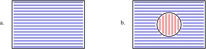
Figure 3: The world-sheet of a 2-string. (a). A purely symmetric string (denoted by horizontal lines). (b). The decay into an antisymmetric string (vertical lines) via an expanding bubble.

The decay rate can be found quasiclassically. The worldsheet of the symmetric string is shown in Fig. 3a. Its decay proceeds via a bubble creation, see Fig. 3b. The worldsheet of the symmetric string is two-dimensional “false vacuum,” while inside the bubble we have a “true vacuum,” i.e. the surface spanned by the anti-symmetric string. The tension difference — in the false vacuum decay problem, the vacuum energy difference — is ${\cal E}\sim\Lambda^{2}N^{-2}$, while the energy $T$ of the bubble boundary (per unit length) is $T\sim\Lambda$. This means that the thin wall approximation is applicable, and the decay rate $\Gamma$ (per unit length of the string per unit time) is [24, 25]

$$\Gamma_{{\rm sym}\to{\rm antisym}}\sim\Lambda^{2}\exp\left(-\frac{\pi\,T^{2}}{{\cal E}}\right)\sim\Lambda^{2}\exp\left(-\gamma\,N^{2}\right)\,,$$ (7.1)

where $\gamma$ is a positive constant of the order of unity. Once the true vacuum domain is created through tunneling, it will expand in real time pushing the boundaries (i.e. the positions of the gluelumps responsible for the conversion) toward the string ends.

The above estimate relies on the assumption that the gluelump energy $\sim\Lambda$. This assumption seems natural, it is hard to imagine any other regime, say, the gluelump mass scaling as $\Lambda/N$. It would be highly desirable to get a better understanding of this issue. Presumably, one should be able to write an effective low-energy theory on the 2-string worldsheet which has two vacua: one stable and one quasi-stable, whose energy density becomes degenerate with that of the stable vacuum in the limit $N\to\infty$. A kink in this theory would describe a gluelump. (See Sect. 10 for a related discussion.) Although the domain wall worldvolume theory of this type is known for quite some time [26], I am aware of no attempts at deriving a QCD $k$-string worldvolume theory along these lines.

8 If $L<L_{\rm crit}$ excited strings may be stable

So far the vast majority of lattice simulations yields string tensions which depend on the particular representation of the probe source rather than on its $N$-ality, with the tension proportional to the Casimir coefficient of the representation at hand. The reason behind this situation may be due to the fact that on lattices so far one deals with a mixture of “wrong” excited strings with just a small admixture of the genuine ground-state $k$ string. The studies of the genuine $k$ strings are hampered by the longevity of the excited strings. As was argued in Sect. 7, excited strings live exponentially long. For, instance, the decay rate of the two-index symmetric string into two-index antisymmetric was estimated as $\Lambda^{2}\exp\left(-\gamma\,N^{2}\right)$.

The above estimate refers to the string of an infinite length. Needless to say, when strings are treated on lattices, they have finite length. If the distance between the probe sources is less than some critical distance $L_{\rm crit}$ the excited string may turn out to be stable, protected against decay into the ground state by energy balance.

Indeed, the energy of the probe configuration depicted in Fig. 1b consists of two parts: the string proper (this energy scales as $L$) and the end-point domains — “bulges” — where the string couples to the color sources (this energy scales as $L^{0}$). The energy of the bulges depends, generally speaking, on the particular representation of the color sources, as well as on the structure of the string proper, i.e. symmetric versus antisymmetric. The bulge connecting the symmetric source with the antisymmetric string is expected to be heavier than that connecting the symmetric source with the symmetric (quasi-stable) string since it absorbs a gluelump. The crucial question is the bulge energy difference in these two cases. If it is $\sim\Lambda$, we need the string to be longer than $\Lambda^{-1}N^{2}$ for the energy gain due to the string decay to overcome the energy loss in the end-point domains. Since the bulge is “locally” coupled to the color source it is conceivable that the bulge energy difference scales as $\sim\Lambda/N$. Then the critical string length is $L_{\rm crit}\mathrel{\hbox to0.0pt{\lower 4.0pt\hbox{\hskip 1.0pt$\sim$}\hss}\raise 1.0pt\hbox{$>$}}\Lambda^{-1}N$.

Thus, “finite-length excited strings” may not be able to relax if the lattice size is smaller than $L_{\rm crit}$. In this case of “short” strings it will be impossible, even in principle, to measure the genuine $k$-string tension no matter how long is the time extension. This circumstance was noted by Gliozzi [27]. I merely adapt his argument within the framework of the large-$N$ analysis.

It is important that $L_{\rm crit}\gg\Lambda^{-1}$. Otherwise framing the discussion in terms of strings would not be appropriate at all.

9 Lattices: what’s happening?

Numerical study of $k$ strings is being pursued, for quite some time, by a number of lattice practitioners, of which I will mention here two groups: one in Italy and one in UK (see e.g. [28, 29]). By and large, the first group finds agreement with the sine law, while the second one obtains results lying between the sine law and the Casimir formula, with somewhat larger errors, which cover both possibilities. A report on the recent progress of the second group can be found in [30]. Lucini et al. obtain string tensions which are somewhat smaller than those measured by the first group, for the same values of lattice parameters, which indicates, generally speaking, that separation of the ground-state string is better in this case. As usual, a potentially dangerous source of systematic errors is the finite-volume correction: both groups rely on the leading bosonic string correction $\sigma_{\rm eff}(L)=\sigma-\pi\,L^{-2}/3$ for extrapolation of their data obtained on a size $L$ lattice to $L\to\infty$. It is not quite clear whether subleading corrections could appreciably distort the ratio $\sigma_{k}/\sigma_{\rm f}$.

In any case, the real question is about the $N\to\infty$ limit, not about $N=4,\,\,6,\,\,8$. A clean way to address this question is to consider, say, $\sigma_{2}/\sigma_{\rm f}$ as a function of $N$, and check whether this ratio receives $1/N$ or $1/N^{2}$ leading corrections. The first analysis of this type was performed in [30], see Eq. (42) and Fig. 15 in this paper. The errors are way too large to provide us with a conclusive answer. To get a conclusive answer large values of $N$ and high accuracy are needed. Experts say they do not expect this issue to be resolved any time soon through this procedure.

At the same time, it is gratifying to note that a number of lattice practitioners stimulated by the pioneering work [31] (where a new method for studying the adjoint string breaking was suggested) became interested in developing new approaches to quasi-stable strings and string decays. Shortly after the original publication [31] this issue was revisited in [32] for the symmetric two-index representation of SU(3), which allowed the authors to explain earlier results that had been reported in [33, 28]. A fresh theoretical analysis along these lines is presented in [27].

Concluding this section let me mention, as a side remark, a landmark achievement marginally related to my current topic: a detailed description of the fundamental string breaking through quark-antiquark pair creation in full QCD was recently obtained in [34].

10 Non-Abelian strings at weak coupling

In this section I describe seemingly the simplest weakly coupled model in which the Meissner effect does take place and leads to formation of non-Abelian chromomagnetic flux tubes. The model supports non-Abelian confined magnetic monopoles. In the dual description the magnetic flux tubes are prototypes of QCD strings. Dualizing the confined magnetic monopoles we get gluelumps (string-attached gluons) which convert a “QCD string” in the excited state to that in the ground state. The decay rate of the excited string to its ground state is suppressed exponentially in $N$, much in the same way as in QCD, see Sect. 7.

The model we will discuss is in a sense minimal. Due to its weak coupling it is fully controllable. One can think of it as of a reference model. It is non-supersymmetric (but can be readily supersymmetrized if necessary). In Part II I will deal with a (slightly broken) supersymmetric version of the same model.

10.1 The bulk structure of the toy four-dimensional Yang–Mills model [14, 15, 16, 5, 6, 17, 18, 19]

The gauge group of the model is SU($N)\times$U(1). Besides SU($N$) and U(1) gauge bosons the model contains $N$ scalar fields charged with respect to U(1) which form $N$ fundamental representations of SU($N$). It is convenient to write these fields in the form of $N\times N$ matrix $\Phi=\{\varphi^{kA}\}$ where $k$ is the SU($N$) gauge index while $A$ is the flavor index,

$$\Phi=\left(\begin{array}[]{cccc}\varphi^{11}&\varphi^{12}&...&\varphi^{1N}\\[5.69054pt] \varphi^{21}&\varphi^{22}&...&\varphi^{2N}\\[5.69054pt] ...&...&...&...\\[5.69054pt] \varphi^{N1}&\varphi^{N2}&...&\varphi^{NN}\end{array}\right)\,.$$ (10.1)

The action of the model has the form

$$S = \int{\rm d}^{4}x\left\{\frac{1}{4g_{2}^{2}}\left(F^{a}_{\mu\nu}\right)^{2}+\frac{1}{4g_{1}^{2}}\left(F_{\mu\nu}\right)^{2}\right.$$ (10.2)

$$+ \left.{\rm Tr}\,(\nabla_{\mu}\Phi)^{\dagger}\,(\nabla^{\mu}\Phi)+\frac{g^{2}_{2}}{2}\left[{\rm Tr}\,\left(\Phi^{\dagger}T^{a}\Phi\right)\right]^{2}+\frac{g^{2}_{1}}{8}\left[{\rm Tr}\,\left(\Phi^{\dagger}\Phi\right)-N\xi\right]^{2}\right\},$$

where $T^{a}$ stands for the generator of the gauge SU($N$),

$$\nabla_{\mu}\,\Phi\equiv\left(\partial_{\mu}-\frac{i}{\sqrt{2N}}\;A_{\mu}-iA^{a}_{\mu}\,T^{a}\right)\Phi\,.$$ (10.3)

The global flavor SU($N$) transformations then act on $\Phi$ from the right. The action (10.2) in fact represents a truncated bosonic sector of the ${\cal N}=2$ supersymmetric model. The last term in the second line forces $\Phi$ to develop a vacuum expectation value (VEV) while the last but one term forces the VEV to be diagonal,

$$\Phi_{\rm vac}=\sqrt{\xi}\,{\rm diag}\,\{1,1,...,1\}\,.$$ (10.4)

To ensure weak coupling one must assume $\xi\gg\Lambda^{2}$.

The vacuum field (10.4) results in the spontaneous breaking of both gauge and flavor SU($N$)’s. A diagonal global SU($N$) survives, however, namely

$${\rm U}(N)_{\rm gauge}\times{\rm SU}(N)_{\rm flavor}\to{\rm SU}(N)_{\rm diag}\,.$$ (10.5)

Thus, color-flavor locking takes place in the vacuum.

This model has a string solution, which I will briefly review now. Since it includes a spontaneously broken gauge U(1), the model supports conventional ANO strings in which one can discard the SU($N$)_gauge part of the action. These are not the strings we are interested in. At first sight the triviality of the homotopy group, $\pi_{1}({\rm SU}(N))=0$, implies that there are no other topologically stable strings. This impression is false. One can combine the $Z_{N}$ center of SU($N$) with the elements $\exp(2\pi ik/N)\in$U(1) to get a topologically stable string solution possessing both windings, in SU($N$) and U(1), namely,

$$\pi_{1}\left({\rm SU}(N)\times{\rm U}(1)/Z_{N}\right)\neq 0\,.$$ (10.6)

It is easy to see that this nontrivial topology amounts to winding of just one element of $\Phi_{\rm vac}$, say, $\varphi^{11}$, or $\varphi^{22}$, etc, for instance

$$\Phi_{\rm string}=\sqrt{\xi}\,{\rm diag}(1,1,...,1,e^{i\alpha(x)})\,,\quad x\to\infty\,,$$ (10.7)

($\alpha$ is the angle of the coordinate $\vec{x}_{\perp}$ in the perpendicular plane.) Such strings are referred to as elementary $Z_{N}$ strings. They are progenitors of the non-Abelian strings. Their tension is $1/N$-th of that of the ANO string, see Eqs. (10.22) and (10.23). The ANO string can be viewed as a bound state of $N$ elementary strings at a certain point in the moduli space.

10.2 Elementary $Z_{N}$ strings

At finite distances from the flux tube center the $Z_{N}$ string solution can be written as [16]

$$\Phi = \left(\begin{array}[]{cccc}\phi(r)&0&...&0\\[5.69054pt] ...&...&...&...\\[5.69054pt] 0&...&\phi(r)&0\\[5.69054pt] 0&0&...&e^{i\alpha}\phi_{N}(r)\end{array}\right),$$ (10.12)

$$A^{{\rm SU}(N)}_{i} = \frac{1}{N}\left(\begin{array}[]{cccc}1&...&0&0\\[5.69054pt] ...&...&...&...\\[5.69054pt] 0&...&1&0\\[5.69054pt] 0&0&...&-(N-1)\end{array}\right)\,\left(\partial_{i}\alpha\right)\left[-1+f_{NA}(r)\right],$$ (10.17)

$$A^{{\rm U}(1)}_{i} = \frac{1}{N}\,\left(\partial_{i}\alpha\right)\left[1-f(r)\right],\qquad A^{{\rm U}(1)}_{0}=A^{{\rm SU}(N)}_{0}=0\,,$$ (10.18)

where $i=1,2$ labels coordinates in the plane orthogonal to the string axis and $r$ and $\alpha$ are the polar coordinates in this plane. The profile functions $\phi(r)$ and $\phi_{N}(r)$ determine the profiles of the scalar fields, while $f_{NA}(r)$ and $f(r)$ determine the SU($N$) and U(1) fields of the string solutions, respectively. These functions satisfy the following rather obvious boundary conditions:

$$\phi_{N}(0)=0,$$

$$f_{NA}(0)=1,\;\;\;f(0)=1\,,$$ (10.19)

at $r=0$, and

$$\phi_{N}(\infty)=\sqrt{\xi},\;\;\;\phi(\infty)=\sqrt{\xi}\,,$$

$$f_{NA}(\infty)=0,\;\;\;\;\;f(\infty)=0$$ (10.20)

at $r=\infty$. Because our model is, in fact, a bosonic reduction of the ${\cal N}=2$ supersymmetric theory, these profile functions satisfy the first-order differential equations,

$$r\frac{d}{{d}r}\,\phi_{N}(r)-\frac{1}{N}\left(f(r)+(N-1)f_{NA}(r)\right)\phi_{N}(r)=0\,,$$

$$r\frac{d}{{d}r}\,\phi(r)-\frac{1}{N}\left(f(r)-f_{NA}(r)\right)\phi(r)=0\,,$$

$$-\frac{1}{r}\,\frac{d}{{d}r}f(r)+\frac{g^{2}_{1}N}{4}\,\left[(N-1)\phi(r)^{2}+\phi_{N}(r)^{2}-N\xi\right]=0\,,$$

$$-\frac{1}{r}\,\frac{d}{{d}r}f_{NA}(r)+\frac{g^{2}_{2}}{2}\,\left[\phi_{N}(r)^{2}-\phi_{2}(r)^{2}\right]=0\,.$$ (10.21)

These equations can be solved numerically. Clearly, the solutions to the first-order equations automatically satisfy the second-order equations of motion.

The tension of the elementary $Z_{N}$ string is

$$T_{1}=2\pi\,\xi\,,$$ (10.22)

to be compared with the tension of the ANO string,

$$T_{\rm ANO}=2\pi\,N\,\xi\,.$$ (10.23)

10.3 Why non-Abelian?

In which sense the elementary $Z_{N}$ strings are progenitors of the bona fide non-Abelian strings? At the classical level they are all degenerate and can be continuously deformed to one another. Indeed, besides trivial translational moduli, they have SU$(N)$ “orientational” moduli corresponding to spontaneous breaking of a non-Abelian symmetry. Indeed, while the “flat” vacuum is SU($N$)_diag symmetric, the solution (10.18) breaks this symmetry down to U(1)$\times$SU$(N-1)$ (at $N>2$). This means that the world-sheet (two-dimensional) theory of the elementary string moduli is the SU($N$)/(U(1)$\times$ SU($N-1$)) sigma model. This is also known as $CP(N-1)$ model.

To obtain the non-Abelian string solution from the $Z_{N}$ string (10.18) we apply the diagonal color-flavor rotation preserving the vacuum (10.4). To this end it is convenient to pass to the singular gauge where the scalar fields have no winding at infinity, while the string flux comes from the vicinity of the origin. In this gauge we have

$$\Phi = U\left(\begin{array}[]{cccc}\phi(r)&0&...&0\\[5.69054pt] ...&...&...&...\\[5.69054pt] 0&...&\phi(r)&0\\[5.69054pt] 0&0&...&\phi_{N}(r)\end{array}\right)U^{-1}\,,$$ (10.28)

$$A^{{\rm SU}(N)}_{i} = \frac{1}{N}\,U\left(\begin{array}[]{cccc}1&...&0&0\\[5.69054pt] ...&...&...&...\\[5.69054pt] 0&...&1&0\\[5.69054pt] 0&0&...&-(N-1)\end{array}\right)U^{-1}\,\left(\partial_{i}\alpha\right)f_{NA}(r)\,,$$ (10.33)

$$A^{{\rm U}(1)}_{i} = -\frac{1}{N}\,\left(\partial_{i}\alpha\right)f(r)\,,\qquad A^{{\rm U}(1)}_{0}=A^{{\rm SU}(N)}_{0}=0\,,$$ (10.34)

where $U$ is a matrix $\in{\rm SU}(N)$. This matrix parametrizes orientational zero modes of the string associated with flux rotation in SU($N$). The presence of these modes makes the string genuinely non-Abelian. Since the diagonal color-flavor symmetry is not broken by the vacuum expectation values (VEV’s) of the scalar fields in the bulk (color-flavor locking) it is physical and has nothing to do with the gauge rotations eaten by the Higgs mechanism. The orientational moduli encoded in the matrix $U$ are not gauge artifacts. The orientational zero modes were first observed in [15, 16].

Thus, at the classical level there is a continuous manifold of non-Abelian strings. The degeneracy is lifted at the quantum level.

10.4 Structure of the string worldsheet theory

As is clear from the string solution (10.34), not each element of the matrix $U$ will give rise to a modulus. The SU($N-1)\times$U(1) subgroup remains unbroken by the string solution under consideration; therefore, as was already mentioned, the moduli space is

$$\frac{{\rm SU}(N)}{{\rm SU}(N-1)\times{\rm U}(1)}\sim CP(N-1)\,.$$ (10.35)

Keeping this in mind we parametrize the matrices entering Eq. (10.34) as follows:

$$\frac{1}{N}\left\{U\left(\begin{array}[]{cccc}1&...&0&0\\[5.69054pt] ...&...&...&...\\[5.69054pt] 0&...&1&0\\[5.69054pt] 0&0&...&-(N-1)\end{array}\right)U^{-1}\right\}^{l}_{p}=-n^{l}n_{p}^{*}+\frac{1}{N}\delta^{l}_{p}\,\,,$$ (10.36)

where $n^{l}$ is a complex vector in the fundamental representation of SU($N$), and

$$n^{*}_{l}n^{l}=1\,,$$ (10.37)

($l,p=1,...,N$ are color indices). One U(1) phase is gauged in the effective sigma model. This gives the correct number of degrees of freedom, namely, $2(N-1)$.

Using this parametrization it is not difficult to obtain [6] an effective (1+1)-dimensional action for the moduli fields $n^{i}$,

$$S^{(1+1)}=2\beta\,\int dt\,dz\,\left\{(\partial_{\alpha}\,n^{*}_{l}\partial_{\alpha}\,n^{l})+(n^{*}_{l}\,\partial_{\alpha}\,n^{l})^{2}\right\}\,,$$ (10.38)

where the coupling constant $\beta$ is given by

$$\beta=\frac{2\pi}{g^{2}_{2}}\,.$$ (10.39)

Equations (10.38) and (10.37) present one of many various parametrizations of CP($N-1$) model which are in use in the literature. It is well known that the continuous degeneracy of the classical vacuum manifold of CP($N-1$) model is lifted at the quantum level (for a pedagogical discussion see e.g. [35]). The quantum vacuum is unique. This means that, unlike $Z_{N}$ strings, our non-Abelian four-dimensional 1-string is unique. This is good. Other aspects are not so good, however.

In two-dimensional CP($N-1$) model there is a large number (of the order of $N$) of quasistable “vacuum states” of the type depicted in Fig. 5. The quasistable vacua of CP($N-1$) model decay into the genuine one with probability $\sim\Lambda^{2}\exp\left(-\gamma\,N\right)$, see Sect. 11.6. In terms of four-dimensional strings this means the existence of a large number of “excited strings” which have nothing to do with the excited $k$-strings since the quasistable vacua of CP($N-1$) model appear for four-dimensional 1-strings, and, moreover, the energy-density spacing is $\Lambda^{2}/N$. Thus, the parallel with QCD is far from being perfect. It is fair to say that we made just the first little step in a long journey which may or may not lead to adequate modeling of QCD strings at weak coupling.

Note that at large $N$ the worldsheet CP($N-1$) model is solvable. Supersymmetrization of the model which will be needed in Part II can be carried out following the program of [5].

Part II: Original

11 $k$-kink confinement in two-dimensional
$CP(N-1)$ models: hints for $k$-string tension?

It is known from the early 1970’s that four-dimensional Yang-Mills theory and two-dimensional O(3) sigma model exhibit remarkable parallels. Just like Yang–Mills theory, O(3) sigma model has asymptotic freedom [36] and instantons [37]. Moreover, $CP(N-1)$ sigma models introduced in Ref. [38, 39] present a parallel to large-$N$ Yang–Mills (YM) theories. The parameter $N$ of $CP(N-1)$ plays the same role as the number of colors in QCD, for instance, $CP(1)$ (equivalent to $O(3)$) is analogous to SU(2) Yang-Mills, $CP(2)$ to SU(3) and so on. The large-$N$ expansion in the sigma models was analyzed in [40, 35], with the conclusion that its structure is very similar to that in YM theories. Finally, 2D supersymmetric $CP(N-1)$ sigma model constructed in [39] is an excellent toy model for 4D supergluodynamics (see e.g. the review paper [41]).

The similarity of the strong-coupling dynamics of four-dimensional Yang–Mills theories and two-dimensional $CP(N-1)$ sigma models is not accidental. As was discussed in Sect. 10 some Yang–Mills models support non-Abelian strings with moduli whose worldsheet interaction is described by $CP(N-1)$. In other words, these YM models are microscopic theories of phenomena whose macroscopic description is given by two-dimensional $CP(N-1)$ models. The Meissner mechanism of confinement translates into quite certain statements concerning kinks in two-dimensional $CP(N-1)$. This explains observations of a number of parallel phenomena in the two classes of theories, 2D and 4D. I want to further exploit this parallelism to pose a question in $CP(N-1)$ model which seemingly escaped theorists’ attention so far.

The issue I want to address is the tension of the configuration with a $k$-kink and $k$-antikink, $k$-kink tension for short. In broken supersymmetric $CP(N-1)$ kinks are confined, much in the same way as quarks in QCD. I will show that the sine formula for the $k$-kink tension emerges in a 2D $CP(N-1)$ model. As usual with toy models, results obtained in toy models, strictly speaking, prove nothing with regards to the real thing. However, with luck, they can provide insights which might be helpful in addressing the original theory. Moreover, although on the one hand toy models are poorer than the original theory (e.g. in the case at hand it is two-dimensional), on the other hand, they may contain free parameters which allow us to fine-tune them so that a variety of dynamical regimes becomes accessible. In the $CP(N-1)$ model we will deal with, several distinct regimes can be realized; one of them is somewhat similar to that of QCD. The interplay between various regimes, including the QCD-like regime, is quite fascinating. Finally, let me mention that $CP(N-1)$ models have a value of their own, unrelated to QCD parallels. To the best of my knowledge, the aspect of the $CP(N-1)$ models I will consider here has never been addressed previously.

11.1 CP($N-1$) model: nonlinear formulation

I start from a brief introduction to 2D supersymmetric ${\rm CP}(N-1)$ models, with emphasis on features that will be exploited in this work.

For any Kähler target space endowed with the metric $G_{\bar{j}\,i}$ the Lagrangian of the ${\cal N}=2$ model is

$${\cal L}_{0}=G_{\bar{j}\,i}\,\partial^{\mu}\bar{\phi}^{\,\bar{j}}\,\partial_{\mu}\phi^{i}+\frac{i}{2}G_{\bar{j}\,i}\,\Psi^{\dagger\bar{j}}\!\stackrel{{\scriptstyle\leftrightarrow}}{{\not\!\!D}}\Psi^{i}+R_{\bar{j}ik\bar{l}}\,\Psi_{L}^{\dagger\bar{j}}\Psi_{L}^{i}\Psi_{R}^{k}\Psi_{R}^{\dagger\bar{l}}\,,$$ (11.1)

where $D_{\mu}$ is the covariant derivative,

$$D_{\mu}\,\Psi^{i}=\partial_{\mu}\,\Psi^{i}+\partial_{\mu}{\phi}^{k}\,\Gamma_{kl}^{i}\,\Psi^{l}\,,$$ (11.2)

$\Gamma$’s stand for the Christoffel symbols, $R_{\bar{j}ik\bar{l}}$ is the curvature tensor, while $\Psi$ denotes a two-component spinor,

$$\Psi=\left(\begin{array}[]{cc}\Psi_{R}\\ \Psi_{L}\end{array}\right),$$ (11.3)

so that the kinetic term of the fermions can be identically rewritten as

$$\frac{i}{2}G_{i\bar{j}}\,\Psi^{\dagger\bar{j}}\!\stackrel{{\scriptstyle\leftrightarrow}}{{\not\!\!D}}\Psi^{i}=\frac{i}{2}G_{i\bar{j}}\left\{\Psi_{L}^{\dagger\bar{j}}\!\stackrel{{\scriptstyle\leftrightarrow}}{{\not\!\!D}}_{R}\Psi_{L}^{i}+\Psi_{R}^{\dagger\bar{j}}\!\stackrel{{\scriptstyle\leftrightarrow}}{{\not\!\!D}}_{L}\Psi_{R}^{i}\right\}\,.$$ (11.4)

The right and left derivatives $\partial_{R,L}$ are

$$\partial_{R}=\partial_{0}-\partial_{1}\,,\qquad\partial_{L}=\partial_{0}+\partial_{1}\,.$$ (11.5)

The metric is obtained from the Kähler potential by differentiation,

$$G_{i\bar{j}}=\frac{\partial}{\partial\phi^{i}}\,\frac{\partial}{\partial\phi^{\dagger\,\bar{j}}}\,K(\phi,\phi^{\dagger})\,.$$ (11.6)

The Kähler potential giving rise to the CP($N-1$) model with the metric in the Fubini-Studi form is

$$K_{{\rm CP}(N-1)}=\frac{2}{g^{2}}\ln\left(1+\sum_{i=1}^{N-1}|\phi^{i}|^{2}\right)\,.$$ (11.7)

Here $g^{2}$ is the dimensionless coupling constant of the model. The CP($N-1$) metric can be written as

$$G_{i\bar{j}}=\frac{2}{g^{2}}\,\delta_{i\bar{j}}\,\frac{1}{\left(1+\sum_{i=1}^{N-1}|\phi^{i}|^{2}\right)}+\left(\phi^{\dagger\,\bar{i}}\,\phi^{j}\right)\mbox{-term}\,.$$ (11.8)

In what follows it will be useful to use the fact [42] that in generic ${\cal N}=2$ compact homogeneous symmetric Kähler sigma models the Ricci tensor $R_{\bar{j}\,i}$ is proportional to the metric. In the case of the CP($N-1$) model

$$R_{\bar{j}\,i}=N\,\frac{g^{2}}{2}G_{i\bar{j}}\,.$$ (11.9)

(In the general case the coefficient $N$ is replaced by $b$, the first — and the only — coefficient in the Gell-Mann–Low function.)

In addition, one can introduce a $\theta$ term which has the following form

$${\cal L}_{\theta}=\frac{i\theta}{2\pi}\,\frac{g^{2}}{2}G_{i\bar{j}}\,\,\varepsilon^{\mu\nu}\partial_{\mu}\phi^{\dagger\,\bar{j}}\partial_{\nu}\phi^{i}\,.$$ (11.10)

If supersymmetry is unbroken, one can always rotate the $\theta$ term away using the anomaly in the axial current; the $\theta$ angle is unobservable. For a detailed review see [43].

As we will discuss shortly, this model has $N$ discrete degenerate vacua. The excitation spectrum of the model consists of kinks interpolating between these vacua.

We will also need to introduce a small supersymmetry (SUSY) breaking. To this end a SUSY-breaking mass term for fermions will be added to the Lagrangian (11.1) and used in due time. The SUSY-breaking mass term can be parametrized as follows:

$${\cal L}_{m}=-i\,mG_{\bar{j}\,i}\,\Psi^{\dagger\bar{j}}_{L}\Psi^{i}_{R}+\mbox{h.c.}=-i\,m\,\frac{2}{Ng^{2}}\left(R_{\bar{j}\,i}\,\Psi^{\dagger\bar{j}}_{L}\Psi^{i}_{R}\right)+\mbox{h.c.}\,,$$ (11.11)

where $m$ is a complex parameter,

$$m=\mu e^{i\alpha}\,,\qquad\mu>0\,,$$ (11.12)

and $Ng^{2}$ is the ’t Hooft coupling. The combination $\mu/g^{2}$ is scale independent, and so is $R\bar{\Psi}\Psi$. If $\mu\neq 0$ the $\theta$ term becomes observable. In fact, it is sufficient to keep only one of two parameters, $\theta\neq 0$ or $\alpha\neq 0$, since by a chiral rotation of the $\Psi$ fields one can always make $m$ real at a price of an appropriate shift of $\theta$. For technical reasons it is slightly more convenient to keep $\alpha$ at zero, while considering $\theta$, the vacuum angle, as a free parameter. From now on we will assume $m$ to be real and positive.

11.2 Linear gauged formulation

Some physical aspects of the $CP(N-1)$ model become more transparent if one uses $N$ constrained fields $n^{i}$ (this is the formulation discussed by Witten [35]). In this language the Lagrangian is built from an $N$-component complex field $n^{i}$ subject to constraint

$$n_{i}^{*}\,n^{i}=1\,,$$ (11.13)

(see e.g. [41]), plus an $N$-component Dirac Fermi field $\psi^{i}$ subject to the constraint

$$n_{i}^{*}\,\psi^{i}=0\,.$$ (11.14)

The Lagrangian has the form

$${\cal L} = \frac{2}{g^{2}}\,\left[\left(\partial_{\mu}-iA_{\mu}\right)n^{*}_{i}\left(\partial_{\mu}+iA_{\mu}\right)n^{i}+\bar{\psi}_{i}(i\not\!\partial-\not\!\!A)\psi^{i}-\frac{1}{2}\left(\sigma^{2}+\pi^{2}\right)\right.$$ (11.15)

$$- \left.\frac{1}{\sqrt{2}}\,\,\bar{\psi}\left(\sigma+i\pi\gamma_{5}\right)\psi-\lambda\left(n^{*}_{i}n^{i}-1\right)+\bar{\chi}n^{*}_{i}\psi^{i}+\bar{\psi}_{i}n^{i}\chi\right],$$

where $\chi$ and $\bar{\chi}$ are Lagrange multiplier fields that enforce the constraint (11.14), $\lambda$ is the Lagrange multiplier enforcing (11.13) while $A_{\mu}$, $\sigma$ and $\pi$ are auxiliary fields which could be eliminated through equations of motion. At the quantum level the above constraints will be gone.

The fields $n_{i}$ and $\psi^{i}$ are $N$-plets. In the formulation (11.1) they are represented by “basic” kinks interpolating between the adjacent vacua of the model, the so-called 1-kinks see below. For this reason, from now on I will refer to the $n^{i}$ quanta as to kinks. Loosely speaking, kinks $\leftrightarrow$ QCD quarks. The $n^{i}$ kink $N$-plet corresponds to the $N$-plet of fundamental quarks.

In this representation the $\theta$ term can be written as

$${\cal L}_{\theta}=\frac{\theta}{2\pi}\,\varepsilon_{\mu\nu}\partial^{\mu}A^{\nu}=\frac{\theta}{2\pi}\,\varepsilon_{\mu\nu}\partial^{\mu}\left(n_{i}^{*}\partial^{\nu}n^{i}\right)\,.$$ (11.16)

Witten showed, by exploiting the $1/N$ expansion to the leading order, that the kink mass is dynamically generated,

$$M_{\rm kink}^{2}=\Lambda^{2}\equiv M_{0}^{2}\exp\left(-\frac{8\pi}{Ng^{2}}\right).$$ (11.17)

Here $M_{0}$ is the ultraviolet cut off and $g^{2}$ is the bare coupling constant. The combination $Ng^{2}$ is nothing but the ’t Hooft constant that does not scale with $N$. As a result, $M_{\rm kink}$ scales as $N^{0}$ at large $N$. This result will be confirmed below in a different way.

In the non-supersymmetric version of the $CP(N-1)$ model Witten found that kinks are subject to confinement, the confining potential grows linearly with distance, with the tension suppressed by $1/N$,

$$\sigma\sim\frac{M_{\rm kink}^{2}}{N}\,.$$ (11.18)

In other words, confinement considered by Witten becomes exceedingly weak at large $N$. The kink-antikink system can be described by a non-relativistic Schrödinger-like equation. This regime does not resemble QCD where the string tension does not vanish at $N\to\infty$. Since we are after emulating QCD we will have to look for another regime. In QCD-like regime the string tension should scale as $N^{0}$.

According to Witten’s $1/N$ analysis which has been repeatedly mentioned above [35], in the supersymmetric version of the $CP(N-1)$ model, the tension vanishes; there is no kink confinement. Thus, it is clear that supersymmetry must be broken.

11.3 What did people learn after Witten?

The development which is most relevant for what follows is the determination of the fermion condensate

$$\left\langle i\,\sum_{j,k}R_{\bar{j}\,k}\,\Psi^{\dagger\bar{j}}_{L}\Psi^{k}_{R}\right\rangle\neq 0\,,\qquad j,k=1,2,...,N-1\,,$$ (11.19)

which is the order parameter exhibiting the spontaneous breaking of $Z_{2N}$ symmetry of the $CP(N-1)$ model down to $Z_{2}$. The $Z_{2N}$ is a discrete remnant of the anomalous axial U(1). The condensate (11.19) scales as $N^{1}$. It can be exactly calculated, see e.g. [41], and takes $N$ distinct values, much in the same way as the gluino condensate $\langle{\rm Tr}\lambda\lambda\rangle$ in SU($N$) SYM four-dimensional theory [44]. Namely,

$$\left\langle i\,\sum_{j,k}R_{\bar{j}\,i}\,\Psi^{\dagger\bar{j}}_{L}\Psi^{k}_{R}\right\rangle=-N\Lambda\exp\left(\frac{2\pi\,i\,k}{N}+i\frac{\theta}{N}\right)\,,\qquad k=0,1,...N-1\,,$$ (11.20)

where $\Lambda$ is the scale parameter, see (11.17). Equation (11.20) refers to arbitrary $\theta$. The dependence on $\theta/N$, in conjunction with the physical $2\pi$ periodicity in $\theta$, prompts us that in the model at hand there are $N$ vacua. In fact, the fermion condensate (11.20) is the order parameter; it labels $N$ discrete supersymmetric vacua of the $CP(N-1)$ model, see Fig. 4. Needless to say, in all vacua the energy density vanishes as a consequence of supersymmetry.

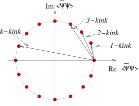
Figure 4: The fermion condensate $\left\langle i\,R_{\bar{j}\,i}\,\bar{\Psi}^{\bar{j}}_{L}\Psi^{i}_{R}\right\rangle$ is the order parameter labeling distinct vacua in $CP(N-1)$ model (the example shown corresponds to $N=16$).

The second relevant development is the fact [45] (see also [35, 46]) that the above operator appears as an anomalous central charge in the superalgebra,

$$\{Q_{R}^{\dagger}\,,\,Q_{L}\} = \frac{i}{2\pi}\int dx\,\partial_{x}\left(R_{i\bar{j}}\,\Psi_{R}^{\dagger\bar{j}}\Psi_{L}^{i}\right)\,,$$

$$\{Q_{L}^{\dagger}\,,\,Q_{R}\} = -\frac{i}{2\pi}\int dx\,\partial_{x}\left(R_{i\bar{j}}\,\Psi_{L}^{\dagger\bar{j}}\Psi_{R}^{i}\right)\,.$$ (11.21)

This is an anomaly, since the central charge is not seen at the classical level. Again, this anomaly is in one-to-one correspondence with a similar anomaly of 4D SYM theory [47].

The presence of the central charge on the right-hand side of Eq. (11.21) implies that there are BPS-saturated kinks interpolating between the distinct vacua, with the masses

$$M_{\rm fi\,\,kink}=\frac{1}{2\pi}\left|\left\langle i\,R_{\bar{j}\,i}\,\Psi^{\dagger\bar{j}}_{L}\Psi^{i}_{R}\right\rangle_{\rm f}-\left\langle i\,R_{\bar{j}\,i}\,\Psi^{\dagger\bar{j}}_{L}\Psi^{i}_{R}\right\rangle_{\rm i}\right|\,,$$ (11.22)

where the subscripts i and f mark the initial and final vacua between which the given kink interpolates. These kinks comprise the physical spectrum of the model. In fact, as is clearly seen from Eqs. (11.22) and (11.20), the kink mass does not depend on specific i and f, but, rather, on the difference f–i.

11.4 $k$-kinks

Taking into account Eq. (11.20) we conclude that the mass of the $k$-kink, i.e. the kink interpolating between $|{\rm vac}\rangle_{i}$ and $|{\rm vac}\rangle_{i+k}$, is

$$M_{k}=(2\pi)^{-1}\,2N\Lambda\sin\left(\frac{\pi k}{N}\right)\,.$$ (11.23)

Although the notion of the $k$-kink is self-evident, a somewhat more specific definition will not hurt. We will assume that the initial and final vacua are fixed. For, instance, let us choose as our initial vacuum that with $k=0$ (the right-most point in Fig.  4 assuming $\theta=0$). If the final vacuum has $k=1$ (the nearest-neighbor vacuum) then we will refer to the corresponding interpolation as to the 1-kink. If the final vacuum has $k=-1$, this is 1-antikink. If $k=\pm 2$ in the final vacuum (the next-to-nearest neighbor) we deal with 2-kinks, and so on. The interpolation in the anti-clock-wise direction will be referred to as kink; the anti-kink interpolates in the clock-wise direction.

The 1-kink is basic, its mass is

$$M_{1}=(2\pi)^{-1}\,2N\Lambda\sin\left(\frac{\pi}{N}\right)\to\Lambda\,,$$ (11.24)

at $N\to\infty$. The 1-kinks are in one-to-one correspondence with the fields $n^{i}$ used in Witten’s work. The mass of the $k$-kink is smaller than $k$ times the mass of the 1-kink, by terms of the order of $1/N^{2}$,

$$M_{k}-kM_{1}=-\Lambda\,\,\frac{\pi^{2}}{6N^{2}}\,k(k^{2}-1)+O(N^{-4})\,.$$ (11.25)

Thus, the $k$-kinks can be viewed as bound states of the 1-kinks. Note that these are not the bound states discussed by Witten, as the latter are of different nature (short-range vs. long-range attractive force). We will return to explaining this point later. In Witten’s approximation only 1-kinks ($n,\,n^{*}$ fields) could be seen.

It is instructive to discuss multiplicity of $k$-kinks, which will be helpful in deciding to which representations the $k$-kinks belong. As we already know, 1-kinks have multiplicity $N$, they form an $N$-plet. The multiplicities of $k$-kinks for arbitrary $k$ were analyzed in [26] (see also [48]). If the initial and final vacua i, f are fixed the multiplicity of the $k$-kinks is [26]

$$\nu_{k}=\frac{N!}{k!(N-k)!}\,.$$ (11.26)

This is consistent with the statement that $k$-kinks are bound states of $k$ fields $n^{i}$ of fully antisymmetric type,

$$n^{[i_{1}}n^{i_{2}}...\,n^{i_{k}]}\,.$$

Thus, if 1-kinks are analogs of fundamental quarks in QCD, the $k$-kinks emulate $k$-index ($N$-ality $k$) antisymmetric representation.

In the supersymmetric $CP(N-1)$ model, if one considers a $k$-kink at the point $x$ and antikink at the point $y$ the interaction between them is short-range, and this pair does not produce a confined system. As was mentioned, if we want to have an analog of the confined quark-antiquark system, we should depart from supersymmetric limit. For instance, Witten’s work demonstrated that 1-kink–1-antikink confinement does take place in nonsupersymmetric $CP(N-1)$ model in the large-$N$ limit. Simple physics lying behind this phenomenon will become transparent shortly. Anticipating the result, I note that the phenomenon occurs because the vacuum degeneracy is lifted [19]. To have a controllable theoretical framework we must guarantee the split between the “former” vacua to be small in the scale of $\Lambda$. This is easy to achieve provided the SUSY-breaking mass term (11.11) is chosen in such a way that $m/g^{2}\ll\Lambda$. In what follows we will limit ourselves to effects of the leading non-trivial order in $m$. In the leading order, i.e. $O(m^{0})$, the result (11.23) for the kink masses stays intact. The kink–antikink tension, which vanishes in the supersymmetric limit, is generated in the order $O(m^{1})$.

11.5 Lifting of the vacuum degeneracy and the choice of vacua

At $m\neq 0$ the vacuum degeneracy is lifted. To order $m^{1}$ the vacuum energy density of the $n$-th vacuum becomes

$${\cal E}_{n}=2{\rm Re}\left\{\frac{2\,m}{Ng^{2}}\left\langle i\,R_{\bar{j}\,i}\,\Psi^{\dagger\bar{j}}_{L}\Psi^{i}_{R}\right\rangle_{n}\right\}=-\frac{4m\Lambda}{g^{2}}\,\cos\left(\frac{\theta}{N}+\frac{2\pi n}{N}\right)\,.$$ (11.27)

To emulate YM theory in a relatively realistic manner we must make sure that our toy model is (i) $CP$ conserving, (ii) the string tension is a $CP$-even quantity and, finally, (iii) the string tension scales as $N^{0}$ in the large-$N$ limit. As has been already mentioned our toy model exhibits a variety of dynamical regimes going beyond the above list. Of this spectrum of dynamical regimes I want to choose the one which meets the requirements (i), (ii) and (iii).

The first requirement implies that $\theta=0$ (in general, $\pi\times$ integer). The second requirement implies that for small $\theta\neq 0$ corrections to the $\theta=0$ string tension are $O(\theta^{2})$, rather than $O(\theta)$. This requirement, in conjunction with the third one, limits possible choices of the initial/final vacua.

Indeed, let us consider the kink interpolating between $|{\rm vac}\rangle_{\ell}$ and $|{\rm vac}\rangle_{\ell^{\prime}}$ with $\ell,\,\,\ell^{\prime}=O(1)$. In this case, as it follows from Eq. (11.27), the energy split

$$|{\cal E}_{\ell}-{\cal E}_{\ell^{\prime}}|\sim 1/N.$$

We will see that the interkink tension is proportional to $|{\cal E}_{\ell}-{\cal E}_{\ell^{\prime}}|$. Thus, this regime is unsuitable for modeling QCD. This regime was analyzed in Ref. [35]. A feeble confinement leads in this case to a nonrelativistic formula for 1-kink–1-antikink pair,

$$M_{\rm bound}=2M_{1}+c\,N^{-2/3}\left(m\Lambda\right)^{1/2}\,,$$

where a constant $c$ depends on the excitation number. I present this formula here only for the sake of completeness.

The correct scaling of the tension, $N^{0}$, is achieved for kinks interpolating between the vacua with

$$n=\frac{N}{4}\pm\ell\,,\qquad\ell=O(1)\,.$$ (11.28)

We will refer to such kinks as symmetric, keeping in mind the symmetricity of the configuration around $n=N/4$. In principle, one could consider asymmetric kinks interpolating between $n=(N/4)+\ell+\ell^{\prime}$ and $n=(N/4)-\ell+\ell^{\prime}$ too. In this case the tension, having the correct scaling law $N^{0}$, violates the requirement (ii).

For the symmetric choice (11.28)

$${\cal E}_{(N/4)+\ell}-{\cal E}_{(N/4)-\ell}=\frac{8m\Lambda}{g^{2}}\,\sin\left(\frac{2\pi\ell}{N}\right)\cos\left(\frac{\theta}{N}\right)=\frac{8m\Lambda}{g^{2}}\,\sin\left(\frac{\pi\,k}{N}\right)\cos\left(\frac{\theta}{N}\right)\,,$$ (11.29)

where $k=2\ell=$ the number of constituents. For the asymmetric choice cos$\,\theta/N$ on the right-hand side would be replaced by cos$\,(2\pi\ell^{\prime}+\theta)/N$; its expansion in $\theta$ would contain a term linear in $\theta$ which would be inappropriate for emulating QCD (condition (ii) is not met).

11.6 Genuine and metastable vacua

Figure 5: The vacuum structure in SUSY-broken $CP(N-1)$ model at $\theta=0$.

Figure 6: The vacuum structure in SUSY-broken $CP(N-1)$ model at $n=\frac{N}{4}+\ell$ where $\ell=\frac{k}{2}$.

If $n\sim 1$ and $N\to\infty$, the spacing between metastable vacua adjacent to the true one ($n=0$) is of the order of $1/N$ as is clearly seen from the expansion of cosine in Eq. (11.27) (with $\theta=0$) and the fact that $g^{2}\sim N^{-1}$ (the height of the barriers scales as $N^{1}$). This is schematically summarized in Fig. 5. The probability of the metastable vacua decay is proportional to $\exp(-N\Lambda/m)$, a straightforward consequence of the false vacuum decay theory [24, 25]. The decay probability vanishes exponentially at $N\to\infty$, somewhat resembling conventional (non-SUSY) 4D Yang-Mills theory [49, 50]. Thus, in this limit each metastable vacuum becomes stable, not only the one corresponding to $n=0$. The fact that the increment of the vacuum energies scales as $1/N$ in this regime is responsible for the factor $N$ in the exponent.

Of more interest to us is the regime (11.28). The pattern of ${\cal E}_{(N/4)+\ell}$ in this regime is given by

$${\cal E}_{(N/4)+\ell}=\frac{4m\Lambda}{g^{2}}\,\sin\left(\frac{2\pi\ell}{N}\right)$$ (11.30)

(at $\theta=0$) and schematically depicted in Fig. 6. In this case the point $\ell=0$ does not correspond to the absolutely stable minimum; rather, the $\ell=0$ state is metastable, as well as all neighboring minima lying in the vicinity of $\ell=0$, say, $\ell=\pm 1,\,\pm 2,$ etc. The increment of the vacuum energy density in the subsequent metastable minima is $O(N^{0}\,m\Lambda)$. The suppression factor in the probability of the metastable vacuum decays becomes

$$N^{-1}\exp(-\Lambda/m)\,.$$

The large-$N$ suppression shows up only in the pre-exponent. Not to break the applicability of the approximation used, we need to keep the SUSY-breaking parameter $m$ small, i.e. $\Lambda/m\gg 1$. This ensures that the suppressing exponent is operative, and the metastable vacua under consideration are in fact stable. Since $m$ is in our hands, this is always doable. It is of paramount importance that the increment of the vacuum energy in the subsequent minima is $O(N^{0})$ in this regime. This translates in the statement $\sigma=O(N^{0})$.

11.7 $k$-kink tension

Now we are fully prepared to consider $k$-kink–$k$-antikink confinement in a QCD-like regime. Let us consider a $k$-kink interpolating between $|{\rm vac}\rangle_{(N/4)-\ell}$ and $|{\rm vac}\rangle_{(N/4)+\ell}$, with $k=2\ell$ on the right, with the corresponding antikink on the left. Schematically this configuration is depicted in Fig. 7.

Figure 7: A $k$-kink separated from $k$-antikink by distance $L$.

The vacuum energy density in the interval between the kinks is higher than that outside,

$$\Delta{\cal E}=\frac{8m\Lambda}{g^{2}}\,\sin\left(\frac{\pi\,k}{N}\right)\,.$$ (11.31)

At large $L$ the overall energy of the configuration depicted in Fig. 7 behaves as

$$\Delta{\cal E}\,L+2M_{k}\,.$$ (11.32)

From this we conclude that the tension of the string confining the $k$-kinks is

$$\sigma_{k}=\frac{8m\Lambda}{g^{2}}\,\sin\left(\frac{\pi\,k}{N}\right).$$ (11.33)

At large $N$ this tension is $N$ independent (remember, $g^{-2}\sim N$), just like it is $N$ independent in QCD. One should remember that the combination $m/g^{2}$ is renormalization-group invariant.

Using Eq. (11.23) one can rewrite the same expression as

$$\sigma_{k}=(8\pi m/Ng^{2})M_{k}\,.$$ (11.34)

Since $m$ is arbitrarily small, confinement is weak (but not suppressed by $1/N$), and the $k$-kinks at the string ends can be viewed as static sources, analogs of the probe QCD quarks in the $k$-index antisymmetric representation of color. It is remarkable that the $k$-kink tension follows the exact sine formula!

I hasten to add a few words about a limitation of this parallel, the presence of two dimensionful parameters, $m$ and $\Lambda$, as opposed to the only parameter $\Lambda$ of YM theory. To keep valid approximations vital for our consideration, one must insist that $m\ll\Lambda$. As supersymmetry breaking increases, and $m$ approaches $\Lambda$, theoretical control erodes, and is finally lost at $m\sim\Lambda$.

One can ask what happens if one interchanges the position of the $k$-kinks in Fig. 7. This would amount to the substitution $\ell\to-\ell$, resulting — formally — in the sign change of the interkink tension (11.33)! In other words, confinement seems to give place to anticonfinement (linear repulsion). This is the consequence of the fact that the vacua we work with are metastable rather than stable. The latter circumstance was imposed on us: in order to emulate $N$-independent string tension of QCD we had no other choice in the toy model at hand. Two kinks repelling each other in fact describe the process of relaxation of an excited string into a less excited state through production of a pair of lumps. I should remind that these are the “wrong” excited strings, with no analogs in QCD, see the end of Sect. 10.

11.8 Lessons for QCD?

In two-dimensional theory $k$-kinks are confined much in the same way as $k$-quarks in QCD. If we choose a QCD-like regime, with the tension $O(N^{0})$, the “$k$-string” spectrum follows the sign formula. This statement is valid if and only if $m\ll\Lambda$, i.e. supersymmetry breaking is small. (One cannot put $m=0$, however, since in the supersymmetric limit kinks in CP$(N-1)$ model are not confined at all).

This may be the most important lesson. Other analyses which produced the sign formula in four dimensions either rely on supersymmetry directly or also assume that its breaking is somehow suppressed. One may conjecture that the sine law for the $k$-string tension takes place in large-$N$ QCD approximately. A hidden small numerical parameter justifying the approximation may emerge due to a “residual supersymmetry” of QCD. This is not a slip of the tongue. One can argue [51] that pure gluodynamics has something like rudimentary supersymmetry! Elaboration of the nature and accuracy of this approximation remains an open task.

References

- [1] J. Greensite, Prog. Part. Nucl. Phys. 51, 1 (2003) [hep-lat/0301023].
- [2] A. Armoni and M. Shifman, Nucl. Phys. B 664, 233 (2003) [hep-th/0304127].
- [3] A. Armoni and M. Shifman, Nucl. Phys. B 671, 67 (2003) [hep-th/0307020].
- [4] M. R. Douglas and S. H. Shenker, Nucl. Phys. B 447, 271 (1995) [hep-th/9503163].
- [5] M. Shifman and A. Yung, Phys. Rev. D 70, 045004 (2004) [hep-th/0403149].
- [6] A. Gorsky, M. Shifman and A. Yung, Phys. Rev. D 71, 045010 (2005) [hep-th/0412082].
- [7] A.A. Abrikosov, Sov. Phys. JETP, 5, 1174 (1957) [Reprinted in Solitons and Partiles, Eds. C. Rebbi and G. Soliani, (World Scientific, Singapore, 1984), p. 356].
- [8] H. B. Nielsen and P. Olesen, Nucl. Phys. B 61, 45 (1973). [Reprinted in Solitons and Partiles, Eds. C. Rebbi and G. Soliani, (World Scientific, Singapore, 1984), p. 365].
- [9] G. ’t Hooft, Nucl. Phys. B 190, 455 (1981).
- [10] S. Mandelstam, Phys. Rept. 23, 245 (1976).
- [11] N. Seiberg and E. Witten, Nucl. Phys. B 426, 19 (1994), (E) B 430, 485 (1994) [hep-th/9407087]; Nucl. Phys. B 431, 484 (1994) [hep-th/9408099].
- [12] A. Hanany, M. J. Strassler and A. Zaffaroni, Nucl. Phys. B 513, 87 (1998) [hep-th/9707244].
- [13] M. J. Strassler, Millenial Messages for QCD from the Superworld and from the String, in At the Frontier of Particle Physics/Handbook of QCD, Ed. M. Shifman, (World Scientific, Singapore, 2001), Vol. 3, p. 1859.
- [14] M. Shifman and A. Yung, Phys. Rev. D 67, 125007 (2003) [hep-th/0212293]; Phys. Rev. D 70, 025013 (2004) [hep-th/0312257].
- [15] A. Hanany and D. Tong, JHEP 0307, 037 (2003) [hep-th/0306150].
- [16] R. Auzzi, S. Bolognesi, J. Evslin, K. Konishi and A. Yung, Nucl. Phys. B 673, 187 (2003) [hep-th/0307287].
- [17] D. Tong, Phys. Rev. D 69, 065003 (2004) [hep-th/0307302].
- [18] A. Hanany and D. Tong, JHEP 0404, 066 (2004) [hep-th/0403158].
- [19] V. Markov, A. Marshakov and A. Yung, Nucl. Phys. B 709, 267 (2005) [hep-th/0408235].
- [20] J. M. Maldacena and C. Nuñez, Phys. Rev. Lett. 86, 588 (2001) [hep-th/0008001].
- [21] C. P. Herzog and I. R. Klebanov, Phys. Lett. B 526, 388 (2002) [hep-th/0111078].
- [22] I. R. Klebanov and M. J. Strassler, JHEP 0008, 052 (2000) [hep-th/0007191].
- [23] A. Butti, M. Graña, R. Minasian, M. Petrini and A. Zaffaroni, JHEP 0503, 069 (2005) [hep-th/0412187].
- [24] I. Y. Kobzarev, L. B. Okun and M. B. Voloshin, Yad. Fiz. 20, 1229 (1974) [Sov. J. Nucl. Phys. 20, 644 (1975)].
- [25] M. B. Voloshin, False vacuum decay, Lecture given at International School of Subnuclear Physics: Vacuum and Vacua: the Physics of Nothing, Erice, Italy, July 1995, in Vacuum and vacua: the physics of nothing, Ed. A. Zichichi (World Scientific, Singapore, 1996), p. 88–124.
- [26] B. S. Acharya and C. Vafa, On domain walls of N = 1 supersymmetric Yang-Mills in four dimensions, hep-th/0103011.
- [27] F. Gliozzi, JHEP 0508, 063 (2005) [hep-th/0507016]; Screening of sources in higher representations of SU(N) gauge theories at zero and finite temperature, hep-lat/0509085.
- [28] L. Del Debbio, H. Panagopoulos, P. Rossi and E. Vicari, JHEP 0201, 009 (2002) [hep-th/0111090].
- [29] B. Lucini and M. Teper, Phys. Rev. D 64, 105019 (2001) [hep-lat/0107007].
- [30] B. Lucini, M. Teper and U. Wenger, JHEP 0406, 012 (2004) [hep-lat/0404008].
- [31] S. Kratochvila and P. de Forcrand, Nucl. Phys. B 671, 103 (2003) [hep-lat/0306011].
- [32] L. Del Debbio, H. Panagopoulos and E. Vicari, JHEP 0309, 034 (2003) [hep-lat/0308012].
- [33] L. Del Debbio, H. Panagopoulos, P. Rossi and E. Vicari, Phys. Rev. D 65, 021501 (2002) [hep-th/0106185].
- [34] G. S. Bali, H. Neff, T. Duessel, T. Lippert and K. Schilling [SESAM Collaboration], Phys. Rev. D 71, 114513 (2005) [hep-lat/0505012].
- [35] E. Witten, Nucl. Phys. B 149, 285 (1979).
- [36] A. M. Polyakov, Phys. Lett. B 59, 79 (1975).
- [37] A. M. Polyakov and A. A. Belavin, JETP Lett. 22, 245 (1975) [Pisma Zh. Eksp. Teor. Fiz. 22, 503 (1975)].
-
[38]
H. Eichenherr,
Nucl. Phys. B 146, 215 (1978);
(E) B 155, 544 (1979);
V. L. Golo and A. M. Perelomov, Lett. Math. Phys. 2, 477 (1978). - [39] E. Cremmer and J. Scherk, Phys. Lett. B 74, 341 (1978).
-
[40]
A. D’Adda, M. Lüscher and P. Di Vecchia,
Nucl. Phys. B 146, 63 (1978);
A. D’Adda, P. Di Vecchia and M. Lüscher, Nucl. Phys. B 152, 125 (1979). - [41] V. A. Novikov, M. A. Shifman, A. I. Vainshtein and V. I. Zakharov, Phys. Rept. 116, 103 (1984).
- [42] See e.g. S. Kobayashi and K. Nomizu, Foundations of Differential Geometry, (Interscience Publishers, New York, 1963–1969), Vols. 1 & 2.
- [43] A. M. Perelomov, Phys. Rept. 146, 135 (1987); 174, 229 (1989).
- [44] M. A. Shifman and A. I. Vainshtein, Nucl. Phys. B 296, 445 (1988).
- [45] A. Losev and M. Shifman, Phys. Rev. D 68, 045006 (2003) [hep-th/0304003].
- [46] M. Shifman, A. Vainshtein, and R. Zwicky, to appear.
- [47] G. Dvali and M. Shifman, Phys. Lett. B396, 64 (1997); (E) B407, 452 (1997) [hep-th/9612128].
- [48] A. Ritz, M. Shifman and A. Vainshtein, Phys. Rev. D 66, 065015 (2002) [hep-th/0205083].
- [49] E. Witten, Phys. Rev. Lett. 81, 2862 (1998) [hep-th/9807109].
- [50] M. Shifman, Phys. Rev. D 59, 021501 (1999) [hep-th/9809184].
- [51] A. Armoni, M. Shifman and G. Veneziano, Phys. Rev. Lett. 91, 191601 (2003) [hep-th/0307097].