3D Relativistic Hydrodynamic Computations Using Lattice-QCD-Inspired Equations of State

Abstract

In this communication, we report results of three-dimensional hydrodynamic computations, by using equations of state with a critical end point as suggested by the lattice QCD. Some of the results are an increase of the multiplicity in the mid-rapidity region and a larger elliptic-flow parameter $v_{2}\,$. We discuss also the effcts of the initial-condition fluctuations and the continuous emission.

1 INTRODUCTION

Nowadays, it is widely accepted that hydrodynamics is a successful approach for describing the bulk of the collective flow in high-energy nuclear collisions [1]. The basic assumption in hydrodynamical models is the local thermal equilibrium. Once this condition is satisfied, all the thermodynamical relations should be valid in each space-time point. The properties of the matter formed in high-energy collisions are then specified by some equations of state (EoS). Thus, one of the main objects of hydrodynamical approach is to determine which are the EoS that consistently reproduce the observed quantities.

In high-energy nucleus-nucleus collisions, one often uses EoS with a first-order phase transition, connecting a high-temperature QGP phase of the system with a low-temperature hadronic phase. However, lattice QCD studies showed that the transition line between QGP and hadron phase has a critical end point and for small net baryon surplus the transition is of crossover type [3]. So, we would like to learn what are the consequences of these results on the hydrodynamics and on the observable quantities.

We shall begin showing, in the next Section, how the critical end point could be implemented for the sake of phenomenological computations. Besides the EoS, the ingredients of any hydrodynamic approach are the equations of motion, the initial conditions and some decoupling prescription. In Sec. 3, we shall discuss how the initial conditions are chosen in our studies; then, how we solve the hydrodynamic equations; and finally which is the decoupling prescription. In Sec. 4, we shall show some of the results of our studies. Finally, summaries of conclusions and outlook are given in Sec. 5.

2 PARAMETRIZATION OF EQUATIONS OF STATE

As mentioned above, one often introduces EoS with a first-order phase transition, connecting a QGP phase of the system, usually described by the MIT bag model, with a hadronic phase, depicted as a resonance gas. A detailed account of such EoS may be found, for instance, in [2]. We start from these EoS, in order to get a phenomenological parametrization of those suggested by lattice QCD.

Let us denote by $P_{Q}$ the pressure given by the MIT bag model and $P_{H}$ the one corresponding to the hadronic resonance gas. Given a value $\mu_{b}$ of the baryonic chemical potential, we write for the pressure $P$ the equation (see Figure 1)

$$(P-P_{Q})(P-P_{H})={\delta(\mu_{b})}\,,$$ (1)

where

$$\delta(\mu_{b})=\delta_{0}\exp\left[-(\mu_{b}/\mu_{c})^{2}\right],\quad\quad\hbox{with}\quad\quad\mu_{c}=\hbox{critical chemical potential}.$$ (2)

By solving the equation above and using thermodynamical relations, we obtain

$$P = \lambda P_{H}+(1-\lambda)P_{Q}+\frac{2\delta}{\sqrt{(P_{Q}-P_{H})^{2}+4\delta}}\ ,$$ (3)

$$s = \lambda s_{H}+(1-\lambda)s_{Q}\,,$$ (4)

$$n_{b} = \lambda n_{H}+(1-\lambda)n_{Q}-\frac{2\,(\mu/\mu_{c}^{2})\,\delta}{\sqrt{(P_{Q}-P_{H})^{2}+4\delta}}\ ,$$ (5)

$$\epsilon = \lambda\epsilon_{H}+(1-\lambda)\epsilon_{Q}-\frac{2\,\left[1+(\mu/\mu_{c})^{2}\right]\,\delta}{\sqrt{(P_{Q}-P_{H})^{2}+4\delta}}\ ,$$ (6)

$$\hbox{where}\quad\lambda \equiv {1\over 2}\left[1-(P_{Q}-P_{H})/\sqrt{(P_{Q}-P_{H})^{2}+4\delta}\right]\ .$$ (7)

Observe that if $\delta_{0}=0$, we recover the EoS with the first-order phase transition described above. In the discussion below, we call them 1OPT EoS. As seen in Figure 1, when $\delta(\mu_{b})\not=0$, the transition from hadron phase to QGP is smooth. In the right-hand side of Eq.(1), we

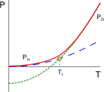
Figure 1: Illustration of Eqs.(1) and (2).

could choose some function which becomes exactly 0 for $\mu_{b}>\mu_{c}$ to guarantee the first-order phase transition there, but for practical purpose this is not necessary. As will be shown below, our choice represented by Eq.(2) is enough. We shall designate the equations of state given above, with $\delta_{0}\not=0$, CP EoS.

Let us compare in Figure 3 below, the temperature dependences of the energy and entropy densities, $\varepsilon$ and $s$, and the pressure $P$, given by the two sets of EoS defined above. One can see that the cross-

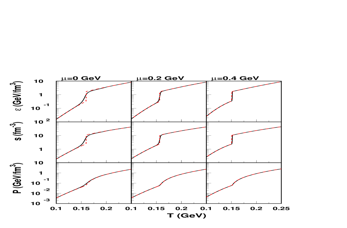
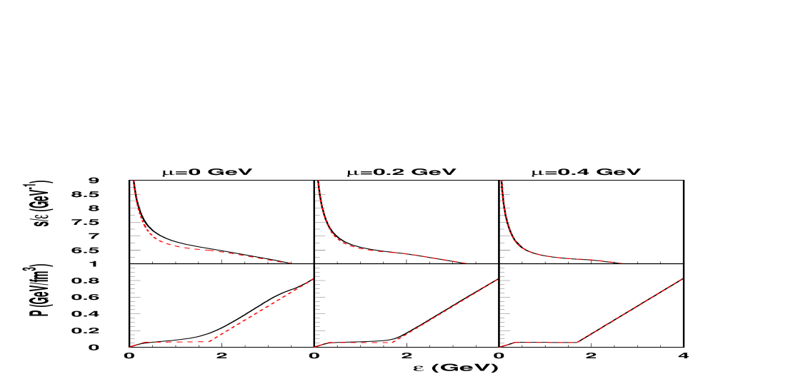
Figure 2: A comparison of $\varepsilon(T)$, $s(T)$ and $P(T)$ as given by our parametrization with a critical point (solid lines) and those with a first-order phase transition (dashed lines).

Figure 3: Plots of $s/\varepsilon$ and $P$ as function of $\varepsilon$ for the two EoS shown in Figure 3.

over behavior is correctly reproduced by our parametrization for CP EoS, while finite jumps in $\varepsilon(T)$ and $s(T)$ are exhibited by 1OPT EoS, when $T$ crosses the transiton temperature. It is also seen, as mentioned above, that at $\mu_{b}\sim 0.4\,$GeV the two EoS are indistinguishable.

Now, since in a real collision what is directly given is the energy distribution at a certain initial time (besides baryon number distribution, charge distribution, strangeness distribution, etc.), whereas the temperature is defined with the use of the former, it would be nice to compare the two sets of EoS, by plotting several quantities as function of $\varepsilon$. We do this in Figure 3. One immediately sees there some remarkable differences between the two sets of EoS: $i\,$) naturally the pressure is not constant for CP EoS in the crossover region; $ii\,$) moreover, the entropy is larger. We will see in Sec.4 that these characteritics affect the observed quantities in non-negligible way.

3 OTHER INGREDIENTS OF OUR HYDRODYNAMIC MODEL

Besides the equations of state, the other ingredients of a hydrodynamic model are the initial conditions, the equations of motion and some decoupling prescription. Here we shall discuss how these elements are chosen in our studies.

3.1 Initial Conditions

In usual hydrodynamic approach, one assumes some highly symmetric and smooth initial conditions (IC). However, since our systems are small, large event-by-event fluctuations are expected in real collisions, so this effect should be taken into account. Remark that this might happen even if the impact parameter could be maintained fixed.

Many simulators, based on microscopic models, e.g. HIJING [4], VNI [5], URASiMA [6], NeXuS [7], $\cdots$, show such event-by-event fluctuations. As an example we show in Figure 4 the energy density for central Au+Au collisions at 130A GeV, given by NeXuS simulator [7], at mid-rapidity. In our approach, we use both fluctuating and averaged IC. Some consequences of such fluctuations have been discussed elsewhere. We shall discuss some others in Sec.4.

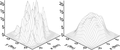
Figure 4: The energy density is plotted in units of GeV/fm³ at the initial instant. Left: one random event. Right: average over 30 random events (corresponding to the smooth initial conditions in the usual hydro approach).

3.2 Equations of Motion

The equations of motion of hydrodynamics are the continuity equations expressing the energy-momentum conservation, the baryon-number conservation, and other conservation laws, corresponding to several charges. Here, for the sake of simplicity, we shall consider only the energy-momentum and the baryon number. Since our IC are entirely arbitrary, without any symmetry, as discussed above, the only way to solve the equations is through numerical computations. We have developed a numerical code called SPheRIO (Smoothed Particle hydrodynamic evolution of Relativistic heavy IOn collisions) [8], based on the so called Smoothed-Paricle Hydrodynamics (SPH) algorithm [9].

3.3 Decoupling Prescription

In hydrodynamic treatment of high-energy nuclear collisions, one often assumes decoupling on a sharply defined hypersurface, usually characterized by a constant temperature $T_{fo}$. We call this Sudden Freeze Out (FO). However, our systems are small, so particles may escape from a layer with thickness comparable with the systems sizes. We have proposed an alternative decoupling prescription that we call Continuous Emission (CE) [10] which, as compared to the usual sudden freeze out, we believe closer to what happens in the actual collisions. We introduce, at each space-time point $x^{\mu}$, a certain momentum-dependent escaping probability

$${\cal P}(x,k)=\exp\left[-\int_{\tau}^{\infty}\rho(x^{\prime})\,\sigma v\;\mathrm{d}\tau^{\prime}\right].$$ (8)

To implement this prescription in our SPheRIO code, we had to introduce some approximation to make the computation practicable. First, we take ${\cal P}$ on the average, i.e.,

$${\cal P}(x,k)\rightarrow\langle{\cal P}(x,k)\rangle\equiv{\cal P}(x)$$ (9)

and then we approximate linearly the density $\rho(x^{\prime})=\alpha\,s(x^{\prime})$ in Eq.(8). Thus,

$${\cal P}(x,k)\rightarrow{\cal P}(x)=\exp\left(-\kappa\,\frac{s^{2}}{|\mathrm{d}s/\mathrm{d}\tau|}\right),$$ (10)

where $\kappa=0.5\,\alpha\,\langle\sigma v\rangle$ is estimated to be 0.3 , corresponding to $\langle\sigma v\rangle\approx$ 2 fm².

We show, in Figure 6, the time ($\tau$) evolution of the probability ${\cal P}$, estimated by this expression, in the mid-rapidity plane for the most central Au+Au collisions at 130 A GeV. For comparison, we show, in Figure 6, the corresponding time evolution of the temperature $T$. One sees that, whereas in Sudden Freeze Out, particles are emitted from a constant $T$ line of Figure 6, in Continuous Emission, they are emitted according to the probability ${\cal P}$, so from a difuse space region and during a larger time interval. It will be shown in Sec. 4 that this difference gives important changes in some observables.

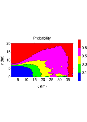
Figure 5: Time evolution of the probability as given by Eq.(10) for the most central Au+Au collisions at 130 A GeV, in the mid-rapidity plane for averaged IC.

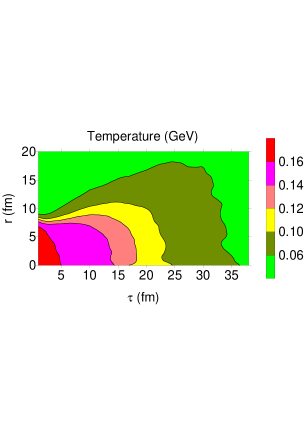
Figure 6: Corresponding time evolution of the temperature.

4 RESULTS

Let us now show results of computation of some observables, as described above, for Au+Au collisions at 200A GeV. We start computing the pseudo-rapidity and the transverse-momentum distributions for charged particles, to fix the parameters. Then, the elliptic-flow parameter $v_{2}$ and HBT radii are computed in fit-parameter free way.

4.1 Pseudo-rapidity distribution

In Sec. 2, we showed that the inclusion of a critical end poit in the first-order phase-transition line increases the entropy per energy, as compared with 1OPT EoS. This means that, given the same total energy, the multiplicity is larger for CP EoS case than for 1OPT EoS one. Figure 8 shows clearly that this happens, especially in the mid-rapidity region.

Now, once the equations of state are chosen, what is the effect of the fluctuating initial conditions for the same decoupling prescription? This effect has already been discussed

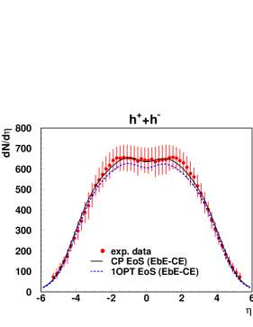
Figure 7: $\eta$ distributions for the most central Au+Au at 200A GeV. A comparison of CP EoS (solid line) vs. 1OPT EoS (dashed line). The data are from PHOBOS Collab.[12].

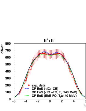
Figure 8: $\eta$ distributions for the most central Au+Au at 200A GeV, computed with CP EoS, with three different combinations of IC and decoupling prescriptions.

earlier [2] and shown in Figure 8, namely, the multiplicity is smaller if the IC fluctuation is taken into account and average computed after the decoupling, as compared with the result obtained with smooth averaged IC. The curve with continuous emission is also shown there, reproducing equally well the data. Here, the parameter $\kappa$ has been fixed as explained in Subsec. 3.3.

4.2 Transverse-Momentum Distribution

As discussed in Sec. 2, since the pressure does not remain constant in the crossover region, we expect that the transverse acceleration is larger for CP EoS, as compared with 1OPT EoS case. In effect, Figure 10 does show that $p_{T}$ distribution is flatter for CP EoS, but the difference is small.

We show, in Figure 10, three different combinations of IC and decoupling prescriptions, corresponding to CP EoS. The curve with the event-by-event fluctuating IC is flatter than the one corresponding to the averaged IC, both with sudden freezeout, probably because the initial expansion in the former is more violent, due to the bumpy structure with high-density blobs, as seen in Figure 4 in this case. The freezeout temperature suggested by $\eta$ and $p_{T}$ distributions turned out to be $T_{f}\simeq 135-140\,$MeV.

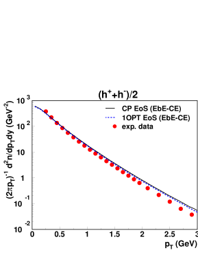
Figure 9: $p_{T}$ distributions for the most central Au+Au at 200A GeV. A comparison of CP EoS (solid line) vs. 1OPT EoS (dashed line). The data are from PHOBOS Collab.[13].

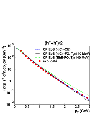
Figure 10: $p_{T}$ distributions for the most central Au+Au at 200A GeV, computed with CP EoS, with three different combinations of IC and decoupling prescriptions.

4.3 Elliptic-Flow Parameter $v_{2}$

Here, we show our results for the pseudo-rapidity distribution of the elliptic-flow parameter $v_{2}$ for Au+Au collisions at 200A GeV. As seen in Figure 12, CP EoS gives larger $v_{2}\,$, as a consequence of larger acceleration in this case as discussed in Sec.2. Notice that the continuous emission makes the curves narrower, as a consequence of earlier emission of particles, so smaller acceleration, at large-$|\eta|$ regions. See more detils in[11]. When the IC fluctuations are taken into account, the resulting fluctuations of $v_{2}$ become large, as seen in Figures 12 and 12. It would be nice to measure such a $v_{2}$ distribution, which would discriminate among several microscopic models for the initial stage of nuclear collisions.

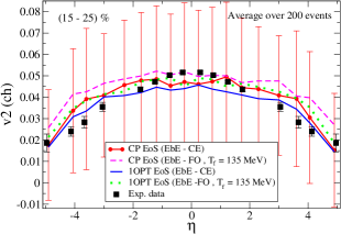
Figure 11: Pseudo-rapidity distribution of $v_{2}$ for charged particles in the centrality $(15-25)$% Au+Au at 200A GeV, computed with event-by-event fluctuating IC. The vertical bars indicate dispersions. The data are from PHOBOS Collab.[14].

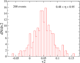
Figure 12: Event-by-event $v_{2}$ distribution in the interval $0.48<\eta<0.95$ and corresponding to the same events as in Figure 12.

4.4 HBT Radii

Here, we show our results for the HBT radii, in Gaussian approximation as used in experimental data analyses, for the most central Au+Au collisions at 200A GeV. As seen in Figures 14, 14 and 16, the differences between CP EoS results and those for 1OPT EoS

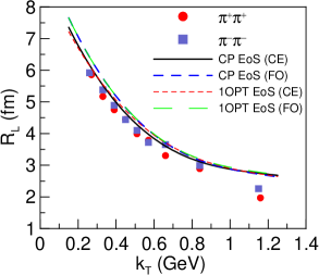
Figure 13: $k_{T}$ depenence of HBT radius $R_{L}$ for pions in the most central Au+Au at 200A GeV, computed with event-by-event fluctuating IC. The data are from PHENIX Collab.[15].

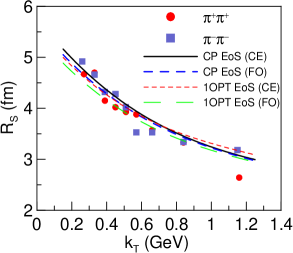
Figure 14: $k_{T}$ depenence of HBT radius $R_{s}$ for pions in the most central Au+Au at 200A GeV, computed with event-by-event fluctuating IC. The data are from PHENIX Collab.[15].

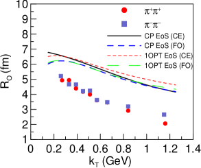
Figure 15: $k_{T}$ depenence of HBT radius $R_{o}$ for pions in the most central Au+Au at 200A GeV, computed with event-by-event fluctuating IC. The data are from PHENIX Collab.[15].

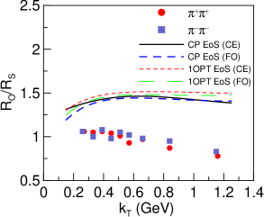
Figure 16: $k_{T}$ depenence of the ratio $R_{o}/R_{s}$ for pions in the most central Au+Au at 200A GeV, computed with event-by-event fluctuating IC. The data are from PHENIX Collab.[15].

are small. This was expected for the case of $R_{L}\,$. For $R_{s}\,$, and especially for $R_{o}\,$, one sees that CP EoS combined with continuous emission gives steeper $k_{T}$ dependence, closer to the data. However, there is still numerical discrepancy in this case.

5 CONCLUSIONS AND OUTLOOKS

In this work, we have introduced a phenomenological parametrization of lattice-QCD-inspired equations of state, which presents a first-order phase transition at large baryonic chemical potential and a crossover behavior at smaller chemical potential. By using the initial conditions generated by NeXuS event simulator and SPheRIO code for solving the hydrodynamic equations, some observables were computed and studied the effects of such EoS. Some of the conclusions are:

1. The multiplicity becomes larger for these equations of state in the mid-rapidity;

2. The $p_{T}$ distribution becomes flatter. However, the differece is small;

3. Larger $v_{2}\,$. Continuous Emission makes the $\eta$ distribution narrower;

4. HBT radii slightly closer to data.

In our calculations, the effect of the continuous emission on the interacting component has not been taken into account. A more realistic treatment of this effect probably makes $R_{o}$ smaller, because the duration for particle emission becomes smaller in this case. Another improvement we should make is the approximations we used for Eq.(8). Cascade treatment of this part is probably a better alternative.

We acknowledge financial support by FAPESP (04/10619-9, 04/15560-2, 04/13309-0), CAPES/PROBRAL, CNPq, FAPERJ and PRONEX.

References

- [1] B. Müller, these proceedings.
- [2] Y. Hama, T. Kodama and O. Socolowski Jr., Braz. J. Phys. 35 (2005) 24.
- [3] Z. Fodor and S.D. Katz, J. High Energy Phys. 03 (2002) 014; F. Karsh, Nucl. Phys. A 698 (2002) 199; S. Katz, these proceedings.
- [4] M. Gyulassy, D.H. Rischke and B. Zhang, Nucl. Phys. A 613 (1997) 397.
- [5] B.R. Schlei and D. Strotman, Phys. Rev. C C59 (1999) 9.
- [6] S. Daté, K. Kumagai, O. Miyamura, H. Sumiyoshi and Xiao-Ze Zhang, J. Phys. Soc. Japan 64, (1995)766; C. Nonaka, E. Honda and S. Muroya, Eur. J. Phys. C 17 (2000) 663.
- [7] H.J. Drescher, F.M. Liu, S. Ostrapchenko, T. Pierog and K. Werner, Phys. Rev. C65 (2002) 054902.
- [8] C.E. Aguiar, T. Kodama, T. Osada and Y. Hama, J. Phys. G 27 (2001) 75; T. Kodama, C.E. Aguiar, T. Osada and Y. Hama, J. Phys. G 27 (2001) 557.
- [9] L.B. Lucy, Astrophys. J. 82 (1977) 1013; R.A. Gingold and J.J. Monaghan, Mon. Not. R. Astro. Soc. 181 (1977) 375.
- [10] F. Grassi, Y. Hama and T. Kodama, Phys. Lett. B 355 (1996) 9; Z. Phys. C 73 (1996) 153.
- [11] R.P.G. Andrade, F. Grassi, Y. Hama, T. Kodama, O. Socolowski Jr. and B. Tavares, poster presented to Quark Matter 05, to appear in Nukleonika.
- [12] PHOBOS Collaboration, B.B. Back et al., Phys. Rev. Lett. 91 (2003) 052303.
- [13] PHOBOS Collaboration, B.B. Back et al., Phys. Lett. B 578 (2004) 297.
- [14] PHOBOS Collaboration, B.B. Back et al., nucl-ex/0407012.
- [15] PHENIX Collaboration, S.S. Adler et al., Phys. Rev. Lett. 93 (2004) 152302.