On the Probabilistic Interpretation of the Evolution Equations with Pomeron Loops in QCD

Abstract

We study some structural aspects of the evolution equations with Pomeron loops recently derived in QCD at high energy and for a large number of colors, with the purpose of clarifying their probabilistic interpretation. We show that, in spite of their appealing dipolar structure and of the self–duality of the underlying Hamiltonian, these equations cannot be given a meaningful interpretation in terms of a system of dipoles which evolves through dissociation (one dipole splitting into two) and recombination (two dipoles merging into one). The problem comes from the saturation effects, which cannot be described as dipole recombination, not even effectively. We establish this by showing that a (probabilistically meaningful) dipolar evolution in either the target or the projectile wavefunction cannot reproduce the actual evolution equations in QCD.

1 Introduction

Over the last year, an intense activity in the field of high–energy QCD has been triggered by the observations that (i) the gluon number fluctuations at low energy play an important role in the evolution towards gluon saturation with increasing energy [1, 2, 3], and (ii) the relevant fluctuations are in fact missed [4] by the existing approaches to non–linear evolution in QCD at high energy, namely, the Balitsky–JIMWLK equations [5, 6, 7, 8]. To cope with that, new equations have been proposed [4, 9, 10, 11] (see also Refs. [12, 13]), which include the particle number fluctuations together with the saturation effects in the limit where the number of colors $N_{c}$ is large. At the same time, an ambitious program was launched, which aims at generalizing these equations to arbitrary values of $N_{c}$ [14, 15, 16, 17, 18, 19, 20, 21]. This effort led already to some important results — in particular, the recognition [15, 11] of a powerful self–duality property of the high–energy evolution, and the construction of an effective Hamiltonian which is explicitly self–dual [17, 20] —, but the general problem is still under study, and the evolution equations for arbitrary $N_{c}$ are not yet known.

In this paper, we shall restrict ourselves to the large–$N_{c}$ limit and investigate whether the evolution equations proposed in Refs. [4, 9] can be given a probabilistic interpretation in the sense of the dipole picture. To motivate our search, let us remind here that most of the modern approaches to high–energy evolution in QCD have an underlying probabilistic structure, which makes their physical interpretation transparent and greatly simplifies the analysis of their consequences, via analytic or numerical techniques.

Specifically, the color dipole picture introduced by Mueller [22, 23, 24] describes the BFKL evolution [25] at large $N_{c}$ (including the particle number fluctuations alluded to above) as a classical Markovian process in which a system of dipoles evolves through dipole splitting. This manifest probabilistic interpretation has enabled Salam to build up a Monte–Carlo code allowing for numerical studies of the dipole evolution [26]. The dipole picture is also underlying the derivation by Kovchegov [27] of the non–linear Balitsky–Kovchegov (BK) equation. Recently, this derivation has been extended, by Levin and Lublinsky [28], to the large–$N_{c}$ version of the Balitsky–JIMWLK hierarchy.

Similarly, the color glass condensate formalism [29, 7, 30], which aims at a description of the high density environment at, or near, saturation, is explicitly formulated in terms of a classical probability distribution, which evolves with increasing energy according to a functional Fokker–Planck equation, the JIMWLK equation [6, 7, 8]. The basic microscopic process at work here (in addition to BFKL evolution) is gluon recombination : the JIMWLK Hamiltonian includes vertices for $n\to 2$ gluon merging with $n>2$, which lead to gluon saturation at high energy. The stochastic nature of the JIMWLK evolution is most clearly exhibited by its reformulation as a Langevin equation describing a random walk in the space of Wilson lines [31]. This is also the most convenient formulation for numerical studies, as demonstrated by the analysis in Ref. [32].

Note that the color dipole picture can be also formulated as a “color glass” [24, 10], but the ensuing picture is complementary to the JIMWK evolution: it describes gluon splitting (at large–$N_{c}$), but not also gluon recombination. Clearly, a complete picture should involve a synthesis of these two approaches, but such a synthesis has not been yet achieved in a wavefunction formalism, not even at large $N_{c}$. (See however the recent developments in Refs. [17, 20].) On the other hand, the equations constructed in Refs. [4, 9] propose such a synthesis at the level of the dipole scattering amplitudes (and for large $N_{c}$).

Specifically, these equations refer to the scattering between a projectile which is a set of dipoles and a generic target. As shown in Ref. [11], the equations admit a natural Pomeron interpretation, where the “Pomeron” is the scattering amplitude for an external dipole: They describe the BFKL evolution of the Pomerons together with their interactions: $1\to 2$ Pomeron splitting with the standard dipole vertex [22], and $2\to 1$ Pomeron merging with the “triple–Pomeron vertex” [33, 34]. By iterating these equations, one generates Pomeron loops [23, 4, 11]. So, from now on, we shall refer to them as ‘the evolution equations with Pomeron loops’.

The general structure of these equations alluded to above makes it tempting to search for a probabilistic interpretation in terms of a dipolar reaction–diffusion process, that is, a classical stochastic process in which a collection of dipoles — which represents either the target or the projectile — evolves through splitting and recombination. In what follows we shall briefly explain (leaving the details to the main body of the paper) why such an interpretation is tantalizing in the first place, what would be its benefits in practice, and why it does not really exist. But before we proceed, let us emphasize here that, although our main conclusion is essentially negative — we demonstrate the non–existence of a dipole interpretation —, this result has also positive implications, in the sense that it helps reorienting the efforts towards solving these equations (in particular, via numerical methods), and also towards better understanding the mechanism for gluon saturation. Besides, as we shall see, it helps clarifying some confusion which exists on this point in the literature.

The reason why such an interpretation looks at the first sight appealing is because, taken separately, each of the terms appearing in these equations describes dipole splitting when considered in an appropriate Lorentz frame (and for large $N_{c}$). Specifically, the non–linear terms responsible for unitarity corrections can be seen as dipole splitting in the wavefunction of the projectile [5, 27, 35, 28], whereas the fluctuation terms relevant at low energy represent dipole splitting in the wavefunction of the target [22, 3, 4] (see Sect. 2 below for details). Moreover, the Hamiltonian underlying the Pomeron loop equations, as constructed in Ref. [11], has a remarkable self–duality property [15, 11], which in a given frame interchanges the splitting and the merging pieces of the Hamiltonian. Since the splitting piece has a well–founded dipolar interpretation, it is then tempting to search for a similar interpretation for the merging piece as well.

Indeed, a fully dipolar picture of the evolution of the (projectile or target) wavefunction, involving dipole splitting and merging, would be highly desirable, since very useful in practice. For instance, this would allow one to extend the Monte–Carlo method by Salam [26] up to arbitrarily high energy, and thus facilitate the numerical study of the evolution equations with Pomeron loops. More generally, this would establish an explicit correspondence between high–energy evolution in QCD and some Markovian “reaction–diffusion processes” which are intensively studied in the context of statistical physics (see the textbook [36], and the review papers [37] for more recent developments), from where one could borrow some methods to QCD. Such a correspondence has been already proven to be useful, both at the level of the mean field approximation (the BK equation) [38], where it shed a new light on the ‘geometric scaling’ property of the solution [39, 40, 41, 42], and in analyzing the role of the particle number fluctuations under asymptotic conditions (very high energy and arbitrarily small coupling constant) [3, 4]. But, clearly, it would be extremely useful to extend this correspondence to a more interesting, non–asymptotic, regime, and rely on it in order to translate to QCD the huge experience accumulated with this problem in the context of statistical physics. Last but not least, a wavefunction picture would allow for more general studies, and for the calculation of quantities other than the dipole scattering amplitudes (so like the gluon production in onium–onium scattering, a problem recently addressed in Ref. [43]).

In view of the above, it may seem a little disappointing that such a dipolar picture cannot be actually given, for the reasons that we explain now. The problem comes from the gluon saturation effects, which cannot be described as dipole recombination. This problem can be seen already when trying to introduce saturation effects in the original dipole picture by Mueller [22, 23]: when two dipoles within the same wavefunction are allowed to interact with each other by exchanging gluons, they produce not only dipoles, but also more complicated color states, like quadrupoles. This illustrates the fact that the merging processes responsible for saturation involve a non–trivial flow of color, and thus transcend the dipole picture. The actual theoretical tool for describing saturation, the JIMWLK equation [6, 7, 8], is written in terms of colorful degrees of freedom (gluons and the associated gauge fields), and cannot be directly simplified by taking the large–$N_{c}$ limit [11]. Such a simplification becomes possible only after applying the JIMWLK equation to dipole scattering amplitudes (thus yielding the Balitsky equations [5]); but in that case, the ensuing dipole interpretation refers to the evolution of the projectile through dipole splitting, and not to that of the target towards gluon saturation.

This being said, the suggestive structure of the evolution equations with Pomeron loops alluded to above makes it tempting to search for an effective dipole picture at least, where by “effective” we mean a fictitious dipolar reaction–diffusion process which reproduces the actual equations for the scattering amplitudes without correctly reflecting the microscopic processes at work. (Such an effective picture would be, of course, still suitable for Monte–Carlo simulations.) And as a matter of facts, an effective dipole picture of this type has been recently proposed in Ref. [12], from the point of view of projectile evolution. However, as we shall demonstrate in what follows, that picture is truly ill–defined (it does not describe a physically acceptable reaction–diffusion process), and thus is useless in practice.

The basic problem is that the $2\to 1$ vertex which is supposed to describe dipole recombination within this effective picture (this is the same as the “triple–Pomeron vertex” [33, 34]) has no definite sign, and thus it cannot be given a probabilistic interpretation, as a merging rate per unit rapidity. Very likely, this difficulty reflects the fact that the actual physical mechanism responsible for gluon saturation in QCD is a coherent, collective, effect — the suppression of the rate for gluon emission in the high density regime by strong color fields [8, 44, 45, 31] —, and not a ‘mechanical’ reduction in the number of gluons. And indeed, the effective ‘dipole recombination’ process mentioned above has the property to leave the total number of dipoles in the system unchanged (unlike a real merging mechanism, which always decreases the number of particles).

The above considerations motivate our strategy in this paper, which will be to demonstrate the non–existence of the dipolar picture through explicit construction. Namely, we shall consider a generic dipole–like reaction–diffusion process with arbitrary, non–local, vertices for dipole splitting and merging, and show that the only way for this process to reproduce the actual equations with Pomeron loops in QCD is by choosing the ‘dipole recombination vertex’ as the triple–Pomeron vertex mentioned before. Since the latter has no well–defined probabilistic interpretation, this choice renders the whole process meaningless.

For our analysis to be convincing, we shall repeat it from the points of view of both target and projectile evolution. Indeed, a priori, these two points of view are not fully equivalent with each other, as they involve different ‘factorization schemes’ connecting the scattering amplitudes to the dipole densities:

In the context of target evolution, it will be natural to evaluate the scattering amplitude for an external dipole in the two–gluon exchange approximation. This is motivated by the fact that (i) the dipole picture applies a priori to the dilute target regime, where this approximation is correct indeed, and (ii) when extended to the high–density regime, this approximation leads to a self–dual Hamiltonian [11], which has a suggestive, dipole–like, structure and thus is a natural starting point for the search of a dipole picture.

From the perspective of projectile evolution, on the other hand, there is a priori no need for further approximations (except for the assumed reaction–diffusion process): Following a strategy by Kovchegov [27] (see also Refs. [46, 28, 12]), the equations obeyed by the dipole densities can be exactly mapped onto equations for the scattering amplitudes, including multiple scattering effects to all orders. Yet, the two–gluon exchange approximation strikes back when one attempts to deduce the vertex for dipole recombination by comparison with the actual equations in QCD.

Let us finally note that the lack of a probabilistic interpretation in terms of dipoles does not a priori preclude the existence of alternative stochastic descriptions, involving some more elementary degrees of freedom, so like the gauge field $\alpha_{a}$ to be introduced in Sect. 3. For instance, we have already mentioned that, within the JIMWLK formalism, the saturation processes have a well defined probabilistic interpretation [31], but in terms of gluon fields. Moreover, it is also known that the evolution equations with Pomeron loops can be compactly summarized into a single Langevin equation, with a rather unusual noise term though [9, 10]; this is again suggestive of a classical stochastic process. An approximate version of this Langevin equation [4] has been recently used for numerical studies [47, 48]. It would be very interesting to clarify the precise nature of the stochastic process underlying the equations with Pomeron loops, if any.

The structure of this paper is as follows: In Sect. 2 we briefly review the evolution equations with Pomeron loops together with their physical interpretation from the perspectives of both target and projectile evolution. In Sect. 3, we study the possibility to interpret these equations in terms of dipole evolution in the target. To that aim, we rely on the Hamiltonian formulation introduced in Ref. [11] (to be reviewed in Sect. 3.1), that we first rewrite in terms of dipole operators (in Sect. 3.2) and then use to deduce evolution equations for the dipole densities (in Sect. 3.3). In the next section, these equations are compared to those generated by a genuine reaction–diffusion process. Specifically, in Sect. 4 we introduce the Master equation defining a generic stochastic process with non–local vertices for splitting and recombination, and use it to deduce evolution equations for the dipole densities. (For convenience, the general equations are summarized in the Appendix.) Finally, in Sect. 5, we consider a reaction–diffusion process taking place at the level of the projectile. From the equations for the dipole densities (cf. Sect. 4), we deduce equations for the scattering amplitudes, which are eventually compared to the QCD equations with Pomeron loops.

2 Evolution equations with Pomeron loops

In this section, we shall briefly recall the evolution equations for dipole scattering amplitudes in QCD at high energy and large $N_{c}$, together with their physical interpretation in terms of splitting and merging processes in either the target or the projectile [4, 9, 10].

The relevant equations describe the rapidity evolution of the scattering amplitudes $\langle T^{(\kappa)}\rangle$ for the collision between a system of $\kappa$ dipoles (the ‘projectile’) and a generic hadronic target. The dipoles making up the projectile are assumed to be small enough for their scattering to lie within the scope of perturbation theory. In the course of the evolution, amplitudes $\langle T^{(\kappa)}\rangle$ corresponding to different values of $\kappa$ get mixed with each other, via the gluon splitting and recombination effects. Thus, the equations form an infinite hierarchy, whose general structure can be easily appreciated by inspection of the first two equations. These read [9]

$$\frac{\partial\left\langle T(\bm{x},\bm{y})\right\rangle}{\partial Y}\,=\frac{\bar{\alpha}_{s}}{2\pi}\int\limits_{\bm{z}}\big{[}\cal{M}_{\bm{x}\bm{y}\bm{z}}\otimes\left\langle T(\bm{x},\bm{y})\right\rangle-\cal{M}(\bm{x},\bm{y},\bm{z})\,\left\langle T^{(2)}(\bm{x},\bm{z};\bm{z},\bm{y})\right\rangle\big{]},\vspace{-.5cm}$$ (2.1)

and, respectively,

$$\frac{\partial\left\langle T^{(2)}(\bm{x}_{1},\bm{y}_{1};\bm{x}_{2},\bm{y}_{2})\right\rangle}{\partial Y}\,= \frac{\bar{\alpha}_{s}}{2\pi}\int\limits_{\bm{z}}\Big{\{}\Big{[}\cal{M}_{\bm{x}_{1}\bm{y}_{1}\bm{z}}\otimes\left\langle T^{(2)}(\bm{x}_{1},\bm{y}_{1};\bm{x}_{2},\bm{y}_{2})\right\rangle$$ (2.2)

$$-\cal{M}(\bm{x}_{1},\bm{y}_{1},\bm{z})\,\left\langle T^{(3)}(\bm{x}_{1},\bm{z};\bm{z},\bm{y}_{1};\bm{x}_{2},\bm{y}_{2})\right\rangle\Big{]}+\big{[}1\leftrightarrow 2\,\big{]}\Big{\}}$$

$$+\left(\frac{\alpha_{s}}{2\pi}\right)^{2}\frac{\bar{\alpha}_{s}}{2\pi}\int\limits_{\bm{u},\bm{v}}\cal{R}(\bm{x}_{1},\bm{y}_{1};\bm{x}_{2},\bm{y}_{2}|\bm{u},\bm{v})\,\left\langle T(\bm{u},\bm{v})\right\rangle,\vspace{-.5cm}$$

where $\bar{\alpha}_{s}=\alpha_{s}N_{c}/\pi$, $Y$ is the rapidity gap between the projectile and the target, $\left\langle T(\bm{x},\bm{y})\right\rangle$ is the scattering amplitude for an external quark–antiquark dipole with the quark leg at $\bm{x}$ and the antiquark leg at $\bm{y}$, $\langle T^{(2)}(\bm{x}_{1},\bm{y}_{1};\bm{x}_{2},\bm{y}_{2})\rangle$ refers similarly to two external dipoles with coordinates $(\bm{x}_{1},\bm{y}_{1})$ and $(\bm{x}_{2},\bm{y}_{2})$, respectively, and so forth.

The two kernels $\mathcal{M}$ and $\cal{R}$ which enter the above equations are defined as follows:

$$\mathcal{M}(\bm{x},\bm{y},\bm{z})\,\equiv\,\frac{(\bm{x}-\bm{y})^{2}}{(\bm{x}-\bm{z})^{2}(\bm{y}-\bm{z})^{2}}\,,\vspace{-.5cm}$$ (2.3)

is the dipole kernel [22, 24], which characterizes the differential probability for an elementary dipole $(\bm{x},\bm{y})$ to split into two dipoles $(\bm{x},\bm{z})$ and $(\bm{z},\bm{y})$ per unit rapidity. We have also introduced the shorthand notation

$$\cal{M}_{\bm{x}\bm{y}\bm{z}}\otimes f(\bm{x},\bm{y})\equiv\cal{M}(\bm{x},\bm{y},\bm{z})[-f(\bm{x},\bm{y})+f(\bm{x},\bm{z})+f(\bm{z},\bm{y})].\vspace{-.5cm}$$ (2.4)

Furthermore, $\cal{R}$ is the triple–Pomeron kernel (this name will be explained in Sect. 5.1)

$$\cal{R}(\bm{x}_{1},\bm{y}_{1};\bm{x}_{2},\bm{y}_{2}|\bm{u},\bm{v})\,\equiv\,\int\limits_{\bm{z}}\nabla_{\bm{u}}^{2}\nabla_{\bm{v}}^{2}\big{[}\mathcal{M}(\bm{u},\bm{v},\bm{z})\,\cal{A}_{0}(\bm{x}_{1},\bm{y}_{1}|\bm{u},\bm{z})\,\cal{A}_{0}(\bm{x}_{2},\bm{y}_{2}|\bm{z},\bm{v})\,\big{]},\vspace{-.5cm}$$ (2.5)

where $\alpha_{s}^{2}\,\cal{A}_{0}$ is (up to a sign) the amplitude for dipole–dipole scattering in the two–gluon exchange approximation and for large $N_{c}$, with

$$\cal{A}_{0}(\bm{x},\bm{y}|\bm{u},\bm{v})\,=\,\frac{1}{8}\left[\ln\frac{(\bm{x}-\bm{v})^{2}(\bm{y}-\bm{u})^{2}}{(\bm{x}-\bm{u})^{2}(\bm{y}-\bm{v})^{2}}\right]^{2}.\vspace{-.5cm}$$ (2.6)

The general structure of the higher equations in this hierarchy can now be easily understood : The amplitude for $\kappa$ dipoles with $\kappa\geq 2$ is coupled to the one for $\kappa\!-\!1$ dipoles, to that for $\kappa$ dipoles, and to that for $\kappa\!+\!1$ dipoles. For more clarity, in what follows we shall refer to these three types of terms as the fluctuation terms, the (normal) BFKL terms, and the unitarity corrections, respectively. (These names should become clear from the subsequent discussion.) If one ignores the fluctuation terms, which are formally suppressed by an additional factor of $\alpha_{s}^{2}$ (see, e.g., the last term in Eq. (2.2)), then the above hierarchy boils down to the large–$N_{c}$ version of the Balitsky–JIMWLK hierarchy [5, 35, 28]. However, as pointed out in Refs. [2, 3, 4], the fluctuation terms are in fact leading–order effects whenever the target is so dilute (or, equivalently, the external dipole $(\bm{x},\bm{y})$ is so small) that $\left\langle T(\bm{x},\bm{y})\right\rangle\mathrel{\hbox to0.0pt{\raise 2.20013pt\hbox{$<$}\hss}{\lower 2.20013pt\hbox{$\sim$}}}\alpha_{s}^{2}$. Note also that $T=1$ is a fixed point of the evolution described by these equations, which physically corresponds to the ‘black disk’ limit at high energy.

The above equations are invariant under a Lorentz boost along the collision axis [11], but the physical interpretation of the various terms depends upon the frame in which we visualize the evolution. As mentioned in the Introduction, it is always possible to choose the frame in such a way that a given term corresponds to dipole splitting.

Namely, the BFKL terms and the unitarity corrections (that is, all the terms in Eqs. (2.1)–(2.2) except for the last term in Eq. (2.2)) can be interpreted as dipole splitting in the evolution of the projectile : If the rapidity increment $dY$ is given to the projectile, one of the $\kappa$ original dipoles there splits into two new dipoles, which then scatter off the target. From this perspective, the BFKL terms $\sim T^{(\kappa)}$ correspond to the separate scattering of the daughter dipoles (plus virtual corrections), whereas the unitarity effects $\sim T^{(\kappa+1)}$ are rather associated with their simultaneous scattering.

Alternatively, the rapidity increment $dY$ can be given to the target, in which case it is the fluctuation term $\sim T^{(\kappa-1)}$ (e.g., the last term in Eq. (2.2)) which admits a simple, dipolar, interpretation [4]: In the weak scattering regime where such fluctuations are truly important, the target is dilute and can be itself described, within the large–$N_{c}$ approximation, as a collection of dipoles which evolve through dipole splitting [22, 24, 10]. Then the last term in Eq. (2.2) describes the splitting of the target dipole $(\bm{u},\bm{v})$ into two new dipoles $(\bm{u},\bm{z})$ and $(\bm{z},\bm{v})$, which then scatter off the external dipoles $(\bm{x}_{1},\bm{y}_{1})$ and $(\bm{x}_{2},\bm{y}_{2})$ via twice two–gluon exchange. This interpretation becomes perhaps more transparent after performing some integrations by parts to rewrite this term as

$$\frac{\partial\left\langle T^{(2)}(\bm{x}_{1},\bm{y}_{1};\bm{x}_{2},\bm{y}_{2})\right\rangle}{\partial Y}\,\bigg{|}_{\rm fluct}=\left(\frac{\alpha_{s}}{2\pi}\right)^{2}\frac{\bar{\alpha}_{s}}{2\pi}\int\limits_{\bm{u},\bm{v},\bm{z}} \mathcal{M}(\bm{u},\bm{v},\bm{z})\,\cal{A}_{0}(\bm{x}_{1},\bm{y}_{1}|\bm{u},\bm{z})\,\cal{A}_{0}(\bm{x}_{2},\bm{y}_{2}|\bm{z},\bm{v})\,$$

$$\times\nabla_{\bm{u}}^{2}\nabla_{\bm{v}}^{2}\,\left\langle T(\bm{u},\bm{v})\right\rangle,$$ (2.7)

(this is the original form of this term in Ref. [9]) and then observing that, in the dilute regime, $\nabla_{\bm{u}}^{2}\nabla_{\bm{v}}^{2}\left\langle T(\bm{u},\bm{v})\right\rangle$ is proportional to the average dipole number density in the target $\left\langle n(\bm{u},\bm{v})\right\rangle$, as it will be explained in Sect. 3.2 below.

The BFKL terms too can be understood as dipole splitting in the target [22, 24]. On the other hand, the unitarity corrections do not admit a dipolar interpretation in this frame: From the perspective of target evolution, they rather correspond to saturation effects, that is, to gluon recombination in the target wavefunction. Similarly, the fluctuation terms can be associated with gluon recombination in the projectile wavefunction. We thus arrive at a physical picture in which, in a given frame, some of the terms in the evolution equations at large $N_{c}$ can be directly interpreted as dipole splitting, whereas the other terms correspond (in a less direct way, though) to gluon merging. As anticipated in the Introduction, and it will be explained in detail in what follows, the gluon merging is the process which prevents a fully dipolar interpretation for the evolution equations even at large $N_{c}$.

3 Dipoles in the target

In this section, we shall demonstrate that Eqs. (2.1)–(2.2) for the scattering amplitudes cannot be obtained as the result of a stochastic process involving dipoles in the target. To that aim, we shall start with the Hamiltonian formulation of these equations [11], which in the dilute regime reduces to the original dipole picture by Mueller (in its ‘color glass’ version of Refs. [24, 10]), and thus represents a natural starting point in the search for a dipole interpretation.

3.1 Hamiltonian formulation in the $\alpha$–representation

As shown in [11], the whole hierarchy of evolution equations for dipole scattering amplitudes as presented in Sect. 2 can be derived from the following effective Hamiltonian

$$H=H_{0}+H_{1\to 2}+H_{2\to 1},\vspace{-.5cm}$$ (3.1)

where the three distinct terms correspond, respectively, to BFKL evolution, gluon splitting, and gluon merging in the wavefunction of the target. They are given by :

$$H_{0}=\frac{1}{2N_{c}^{2}}\,\frac{\bar{\alpha}_{s}}{2\pi}\int\limits_{\bm{u},\bm{v},\bm{z}}\cal{M}(\bm{u},\bm{v},\bm{z})\left[\alpha^{a}(\bm{u})-\alpha^{a}(\bm{z})\right][\alpha^{a}(\bm{z})-\alpha^{a}(\bm{v})]\frac{\delta}{\delta\alpha^{b}(\bm{u})}\frac{\delta}{\delta\alpha^{b}(\bm{v})},\vspace{-.5cm}$$ (3.2)

$$H_{1\to 2}=-\frac{g^{2}}{16N_{c}^{3}}\,\frac{\bar{\alpha}_{s}}{2\pi}\int \cal{M}(\bm{u},\bm{v},\bm{z})\cal{G}(\bm{u}_{1}|\bm{u},\bm{z})\cal{G}(\bm{v}_{1}|\bm{u},\bm{z})\cal{G}(\bm{u}_{2}|\bm{z},\bm{v})\cal{G}(\bm{v}_{2}|\bm{z},\bm{v})$$ (3.3)

$$\times\nabla_{\bm{u}}^{2}\nabla_{\bm{v}}^{2}\alpha^{c}(\bm{u})\alpha^{c}(\bm{v})\,\frac{\delta}{\delta\alpha^{a}(\bm{u}_{1})}\frac{\delta}{\delta\alpha^{a}(\bm{v}_{1})}\frac{\delta}{\delta\alpha^{b}(\bm{u}_{2})}\frac{\delta}{\delta\alpha^{b}(\bm{v}_{2})},\vspace{-.5cm}$$

$$H_{2\to 1}=\frac{g^{2}}{16N_{c}^{3}}\frac{\bar{\alpha}_{s}}{2\pi}\!\int\limits_{\bm{u},\bm{v},\bm{z}}\!\!\!\cal{M}(\bm{u},\bm{v},\bm{z})\left[\alpha^{a}(\bm{u})-\alpha^{a}(\bm{z})\right]^{2}[\alpha^{b}(\bm{z})-\alpha^{b}(\bm{v})]^{2}\frac{\delta}{\delta\alpha^{c}(\bm{u})}\frac{\delta}{\delta\alpha^{c}(\bm{v})}.\,\,\vspace{-.5cm}$$ (3.4)

In these equations, $\alpha^{a}(\bm{z})$ is the total color gauge field radiated by color sources within the target (in an appropriate gauge), and the function $\cal{G}(\bm{u}_{1}|\bm{u},\bm{z})$ represents (up to a factor $g\,t^{a}$) the classical field created at $\bm{u}_{1}$ by the elementary dipole $(\bm{u},\bm{z})$:

$$\cal{G}(\bm{u}_{1}|\bm{u},\bm{z})=\frac{1}{4\pi}\ln\frac{(\bm{u}_{1}-\bm{z})^{2}}{(\bm{u}_{1}-\bm{u})^{2}}.\vspace{-.5cm}$$ (3.5)

In what follows, we shall refer to the above form of the effective theory as the “$\alpha$–representation”. The operators $\alpha^{a}(\bm{z})$ and $\delta/\delta\alpha^{a}(\bm{z})$ can be interpreted as ‘Fock–space operators’ which annihilate and create a gluon, respectively. This makes it clear that the above Hamiltonian describes the evolution of the gluon distribution in the target, which proceeds through BFKL evolution ($H_{0}$), $2\to 4$ gluon splitting ($H_{1\to 2}$), and $4\to 2$ gluon merging ($H_{2\to 1}$). From this perspective, the splitting Hamiltonian (3.3) [10] should be more naturally denoted as $H_{2\to 4}$ (and similarly $H_{4\to 2}$ for the merging term (3.4)), but the present notations anticipate the ‘dipolar’ form of the Hamiltonian, to be presented later. The Hamiltonian in Eqs. (3.1)–(3.4) has a remarkable self–duality property [15, 11], to be discussed in Sect. 5.1.

In this representation, the scattering amplitudes for external dipoles are obtained as $\langle T^{(\kappa)}\rangle=\langle\,T(1)T(2)...T(\kappa)\rangle$, where $T\equiv T(\bm{x},\bm{y})$ is the following scattering operator:

$$T(\bm{x},\bm{y})=\frac{g^{2}}{4N_{c}}\,\left[\alpha^{a}(\bm{x})-\alpha^{a}(\bm{y})\right]^{2},\vspace{-.5cm}$$ (3.6)

which appears to describe single scattering in the two–gluon exchange approximation. However, within the present formalism, Eq. (3.6) is to be used in the whole kinematical range, including at high energy where the multiple scattering is important. This is appropriate since the $\alpha$–representation described here is only an effective theory, in which the various microscopic process are not always faithfully depicted, but which reproduces, by construction, the correct evolution equations for the scattering amplitudes (that is, the hierarchy starting with Eqs. (2.1)–(2.2)). Indeed, by using the above formulæ, it is straightforward to check that the Hamiltonian evolution equations

$$\frac{\partial\left\langle T^{(\kappa)}\right\rangle}{\partial Y}=\left\langle H\,T^{(\kappa)}\right\rangle\vspace{-.5cm}$$ (3.7)

generate the expected hierarchy, so long as one neglects contractions which give terms suppressed at large–$N_{c}$. For example, when acting with $\delta^{2}/\delta\alpha^{a}_{\bm{u}_{1}}\delta\alpha^{a}_{\bm{v}_{1}}$ from $H_{1\to 2}$ on the two–dipole scattering operator $T^{(2)}(\bm{x}_{1},\bm{y}_{1};\bm{x}_{2},\bm{y}_{2})$, one should keep in the equation only the terms which are generated when both derivatives act on the same dipole. In that sense, the action of the Hamiltonian is constrained by a large–$N_{c}$ counting rule. Moreover, the Hilbert space for the $\alpha$–representation is also constrained: Because of the assumptions underlying the construction of the Hamiltonian (3.1)–(3.4) (see the discussion in Ref. [11]), this Hamiltonian cannot be used to act on arbitrary operators built with $\alpha$, but only on the operators built with the scattering amplitude (3.6). (Such acceptable operators are gauge invariant in the sense explained in Ref. [49].)

3.2 Hamiltonian theory in the $D$–representation

In the $\alpha$–representation introduced above, the dipolar structure of the Hamiltonian is not explicit. But as we shall explain below, this structure becomes manifest after a change of representation, which has also the advantage to eliminate all the constraints on the Hamiltonian structure that we have previously mentioned.

Specifically, one can reexpress the Hamiltonian and the interesting observables (the scattering amplitudes) in terms of operators which are bilinear in the number of fields $\alpha$ or of functional derivatives $\delta/\delta\alpha$. If $\rho_{a}$ denotes the color charge density in the target, so that

$$-\nabla_{\bm{x}}^{2}\alpha_{a}(\bm{x})=\rho_{a}(\bm{x}),\vspace{-.5cm}$$ (3.8)

then we define the $D$–representation via the following identifications:

$$D_{\bm{x}\bm{y}}=-\frac{1}{g^{2}N_{c}}\,\rho_{a}(\bm{x})\rho_{a}(\bm{y})\quad,\quad\bm{x}\neq\bm{y}\vspace{-.5cm}$$ (3.9)

$$D_{\bm{x}\bm{y}}^{\dagger}=1+\frac{g^{2}}{4N_{c}}\left[\frac{\delta}{\delta\rho^{a}(\bm{x})}-\frac{\delta}{\delta\rho^{a}(\bm{y})}\right]^{2}.\vspace{-.5cm}$$ (3.10)

The notation is slightly abusive, since $D$ and $D^{\dagger}$ are not Hermitian conjugate to each other in any sense, but it is suggestive of the fact that these operators act as creation and annihilation operators for dipoles in the target (see Sect. 3.3 below).

When expressed in terms of $D$ and $D^{\dagger}$, the Hamiltonian takes a rather compact form:

$$H\left[D,D^{\dagger}\right]= \frac{\bar{\alpha}_{s}}{2\pi}\int\limits_{\bm{u},\bm{v},\bm{z}}\cal{M}(\bm{u},\bm{v},\bm{z})\,D_{\bm{u}\bm{v}}\left[-D^{\dagger}_{\bm{u}\bm{v}}+D^{\dagger}_{\bm{u}\bm{z}}D^{\dagger}_{\bm{z}\bm{v}}\right]$$ (3.11)

$$-\frac{1}{2}\left(\frac{\alpha_{s}}{2\pi}\right)^{2}\frac{\bar{\alpha}_{s}}{2\pi}\int\cal{R}(\bm{u}_{1},\bm{v}_{1};\bm{u}_{2},\bm{v}_{2}|\bm{u},\bm{v})\,D_{\bm{u}_{1}\bm{v}_{1}}D_{\bm{u}_{2}\bm{v}_{2}}D^{\dagger}_{\bm{u}\bm{v}}\,,\vspace{-.5cm}$$

where the expression in the first line has been obtained by summing up the BFKL and the splitting pieces of the Hamiltonian, cf. Eqs. (3.2)–(3.3), while that in the second line is a rewriting of the merging Hamiltonian, Eq. (3.4).

Furthermore, the dipole scattering amplitude can be related to the operator $D_{\bm{x}\bm{y}}$ via

$$T(\bm{x},\bm{y})[D]\,=\,\alpha_{s}^{2}\int\limits_{\bm{u},\bm{v}}\cal{A}_{0}(\bm{x},\bm{y}|\bm{u},\bm{v})D_{\bm{u}\bm{v}}\,,\vspace{-.5cm}$$ (3.12)

which follows from Eqs. (3.6), (3.8), and (2.6), together with the condition that the system be globally color neutral: $\int_{\bm{u}}\rho^{a}({\bm{u}})=0$.

To complete the definition of the new representation, one still needs to specify the algebra of the operators $D$ and $D^{\dagger}$. To that aim, we rely on their respective expressions in terms of $\rho$ and $\delta/\delta\rho$, cf. Eqs. (3.9)–(3.10), to conclude that, in the representation in which $D_{\bm{x}\bm{y}}$ is diagonal (i.e., a pure function) and in the large–$N_{c}$ approximation, $D^{\dagger}$ can be represented as a functional derivative with respect to $D$ :

$$D_{\bm{x}\bm{y}}^{\dagger}=1+\frac{\delta}{\delta D_{\bm{x}\bm{y}}}\,,\qquad\mbox{with}\qquad\frac{\delta}{\delta D_{\bm{x}\bm{y}}}\,D_{\bm{u}\bm{v}}\,\equiv\,\frac{1}{2}\left(\delta_{\bm{x}\bm{u}}\delta_{\bm{y}\bm{v}}+\delta_{\bm{x}\bm{v}}\delta_{\bm{y}\bm{u}}\right).\vspace{-.5cm}$$ (3.13)

To understand how this arises, note first that, for $\bm{u}\neq\bm{v}$,

$$\frac{g^{2}}{4N_{c}}\left[\frac{\delta}{\delta\rho^{a}(\bm{x})}-\frac{\delta}{\delta\rho^{a}(\bm{y})}\right]^{2}\,\left(-\frac{1}{g^{2}N_{c}}\,\rho_{a}(\bm{u})\rho_{a}(\bm{v})\right)\,\simeq\,\frac{1}{2}\left(\delta_{\bm{x}\bm{u}}\delta_{\bm{y}\bm{v}}+\delta_{\bm{x}\bm{v}}\delta_{\bm{y}\bm{u}}\right),\vspace{-.5cm}$$ (3.14)

where we have used $N_{c}^{2}-1\simeq N_{c}^{2}$ at large $N_{c}$. Furthermore, if we temporarily return to the $\rho$–representation in Eqs. (3.9)–(3.10) and consider the action of $D^{\dagger}$ on a string of $D$–operators, so like $D_{\bm{x}\bm{y}}^{\dagger}D_{\bm{u}_{1}\bm{v}_{1}}D_{\bm{u}_{2}\bm{v}_{2}}\dots$, then it is clear that the dominant result at large $N_{c}$ is the same as obtained when acting with the functional derivative ${\delta}/{\delta D_{\bm{x}\bm{y}}}$.

Thus, by using the expression (3.11) for the Hamiltonian together with Eq. (3.13) for $D^{\dagger}$, one ensures that the action of $H$ on operators built with $D$ generates only the would–be dominant contributions at large–$N_{c}$. Moreover, the Hilbert space in the $D$–representation is not constrained anymore: Indeed, Eq. (3.12) can be inverted to yield

$$D_{\bm{x}\bm{y}}=\frac{2}{g^{4}}\nabla_{\bm{x}}^{2}\nabla_{\bm{y}}^{2}\,T(\bm{x},\bm{y})\qquad{\rm for}\qquad\bm{x}\neq\bm{y},\vspace{-.5cm}$$ (3.15)

showing that any operator built with $D$ is physically acceptable. Thus, as anticipated, by changing from the $\alpha$ to the $D$–representation we have eliminated all the constraints.

It is now a straightforward exercise to verify that the evolution equations for $\langle D^{(\kappa)}\rangle\equiv\langle D(1)D(2)\dots D(\kappa)\rangle$ generated as:

$$\frac{\partial\langle D^{(\kappa)}\rangle}{\partial Y}=\left\langle H\,D^{(\kappa)}\right\rangle\vspace{-.5cm}$$ (3.16)

lead to the expected equations for the scattering amplitudes after also using Eq. (3.12).

3.3 A dipolar picture and its limitations

We now turn to the dipolar interpretation of the evolution described by the effective Hamiltonian (3.11). As we shall soon discover, such an interpretation is truly meaningful (in the sense of having a probabilistic meaning) only in the dilute regime, where it reduces to the standard dipole picture by Mueller [22, 23]. Namely, for a dilute target, the recombination effects can be ignored and the Hamiltonian (3.11) reduces to the expression in its first line, i.e., $H_{\rm dipole}\equiv H_{0}+H_{1\to 2}$, which is recognized as the ‘color glass’ version of the Hamiltonian generating the dipole picture [24, 10]. As we briefly recall now, the evolution driven by $H_{\rm dipole}$ leads to a probabilistic picture of the target, as a collection of dipoles which evolves through splitting (see Refs. [22, 23, 24, 10, 19] for more details).

Specifically, in the dilute regime, the operators $D^{\dagger}$ and $D$ introduced before can be interpreted as dipole creation and annihilation operators, respectively, with the following commutation relation (at large $N_{c}$):

$$\left[D_{\bm{x}\bm{y}},D^{\dagger}_{\bm{u}\bm{v}}\right]=\frac{1}{2}\left(\delta_{\bm{x}\bm{u}}\delta_{\bm{y}\bm{v}}+\delta_{\bm{x}\bm{v}}\delta_{\bm{y}\bm{u}}\right).\vspace{-.5cm}$$ (3.17)

The target distribution is then obtained by successively acting with the creation operators on the ‘dipole vacuum’, and can be represented as the following ‘color glass weight function’ :

$$Z_{Y}[\rho]\;=\;\sum_{N=1}^{\infty}\,\int d\Gamma_{N}\,P_{N}(\{\bm{u}_{i},\bm{v}_{i}\};Y)\,\prod_{i=1}^{N}D^{\dagger}(\bm{u}_{i},\bm{v}_{i})\,\delta[\rho]\;,\vspace{-.5cm}$$ (3.18)

where the functional distribution $\delta[\rho]$ represents the vacuum (no color charge, and hence no dipole !), $Z_{N}(\{\bm{u}_{i},\bm{v}_{i}\})\equiv\prod_{i=1}^{N}D^{\dagger}(\bm{u}_{i},\bm{v}_{i})\delta[\rho]$ describes a given configuration of $N$ dipoles, $P_{N}(\{\bm{u}_{i},\bm{v}_{i}\};Y)$ is the corresponding probability at rapidity $Y$, and $d\Gamma_{N}$ denotes the measure for the $N$–dipole phase–space: $d{\Gamma}_{N}=(1/N!)\prod_{i=1}^{N}{\rm d}^{2}\bm{u}_{i}{\rm d}^{2}\bm{v}_{i}$.

The ‘weight function’ (3.18) acts as a probability distribution for $\rho_{a}$ when computing target expectation values. For instance:

$$\left\langle D(\bm{x},\bm{y})\right\rangle = \int D[\rho]\,D(\bm{x},\bm{y})\,Z_{Y}[\rho]\,$$ (3.19)

$$= \,\sum_{N=1}^{\infty}\,\int d\Gamma_{N}\,P_{N}(\{\bm{u}_{i},\bm{v}_{i}\};Y)\sum_{i=1}^{N}\delta_{\bm{u}_{i}\bm{x}}\delta_{\bm{v}_{i}\bm{y}}\,\equiv\,\left\langle n(\bm{x},\bm{y})\right\rangle,\vspace{-.5cm}$$

where in writing the second line we have used Eqs. (3.17) and (3.18), and then recognized the definition of the average dipole number density.

In view of the discussion above, the dipole interpretation of the evolution generated by $H_{\rm dipole}$ is quite transparent (cf. the first line of Eq. (3.11)) : The term involving $D_{\bm{u}\bm{v}}D^{\dagger}_{\bm{u}\bm{z}}D^{\dagger}_{\bm{z}\bm{v}}$ describes the splitting of the original dipole $({\bm{u},\bm{v}})$ into two new dipoles $({\bm{u},\bm{z}})$ and $({\bm{z},\bm{v}})$, with a probability density $({\bar{\alpha}_{s}}/{2\pi})\cal{M}(\bm{u},\bm{v},\bm{z})$ per unit of phase–space and per unit rapidity. The other term, proportional to $-D_{\bm{u}\bm{v}}D^{\dagger}_{\bm{u}\bm{v}}$, describes the decrease in the probability that the original dipole remain unchanged after one step in the evolution.

To verify that this probabilistic interpretation is mathematically well founded, one can use $H_{\rm dipole}$ to deduce evolution equations for either the probability densities $P_{N}$, or the dipole number densities $\langle n^{(\kappa)}\rangle\equiv\langle D^{(\kappa)}\rangle$, and then check that the ensuing equations have the structure expected for the Master equations associated with a stochastic process. For the splitting problem described by $H_{\rm dipole}$, both tests have been performed in the literature [26, 24, 4], and they confirm the probabilistic interpretation given above. In what follows we shall follow the second strategy, namely, the one which focuses on the particle densities, but we shall do so in the more general context of an evolution involving both splitting and merging, as generated by the full Hamiltonian in Eq. (3.11).

Indeed, a question which naturally arises at this point is whether one can extend this dipole picture to the high–density regime as well, that is, to the merging piece of the Hamiltonian, as given in the second line of Eq. (3.11). Since proportional to $D_{\bm{u}_{1}\bm{v}_{1}}D_{\bm{u}_{2}\bm{v}_{2}}D^{\dagger}_{\bm{u}\bm{v}}$, is seems natural to interpret this piece as describing the recombination of two dipoles $({\bm{u}_{1},\bm{v}_{1}})$ and $({\bm{u}_{2},\bm{v}_{2}})$ into a single dipole $({\bm{u},\bm{v}})$, with a probability density which is proportional to $\cal{R}(\bm{u}_{1},\bm{v}_{1};\bm{u}_{2},\bm{v}_{2}|\bm{u},\bm{v})$ (and with an overall sign which is not clear yet; this will be clarified in Sect. 4.2). However, a more careful analysis reveals that this interpretation is in fact deceiving, as shown by the following argument: For the probabilistic interpretation to be meaningful, the ‘triple–Pomeron’ kernel $\cal{R}$ must have a definite sign (since a probability density cannot change sign !) However, a brief inspection of Eq. (2.5) reveals that the actual kernel $\cal{R}$ has not a fixed sign. Indeed, using the fact that this kernel is a total derivative and that there are no boundary terms when it is integrated over all the transverse space (as we shall shortly check), we immediately find

$$\int\limits_{\bm{u},\bm{v}}\cal{R}(\bm{u}_{1},\bm{v}_{1};\bm{u}_{2},\bm{v}_{2}|\bm{u},\bm{v})=0,\vspace{-.5cm}$$ (3.20)

showing that the value of the vertex must be negative in some regions of the transverse space, and positive in some others. Clearly, this property prohibits any probabilistic interpretation for the merging vertex in the Hamiltonian (3.11).

At this point, we should stress that the aforementioned sign property of the triple–Pomeron kernel does not entail any sign problem for the fluctuation term in Eq. (2.2), and thus for the actual evolution equations in QCD: Even though $\cal{R}$ has no definite sign, the convolution yielding the last term in Eq. (2.2) is nevertheless positive–definite within the whole kinematical range in which this term is important, that is, in the weak scattering regime. To verify this, it is preferable to rewrite this term as in Eq. (2) and then use the fact, for a dilute target, the quantity $\nabla_{\bm{u}}^{2}\nabla_{\bm{v}}^{2}\left\langle T(\bm{u},\bm{v})\right\rangle$ is positive–semidefinite, since proportional to the average dipole number density (cf. Eqs. (3.15) and (3.19)).

To render the previous arguments more precise, we shall compare in Sect. 4 the equations for the dipole number densities generated by the Hamiltonian (3.11) to those arising from an actual reaction–diffusion process with generic vertices for splitting and recombination. To that aim, let us derive here the corresponding equations in QCD. The ‘dipole number density’ is defined as the expectation value of $D$, cf. Eq. (3.19), and similarly for the higher $\kappa$–body densities (e.g., $\left\langle DD\right\rangle$ is the average pair density, etc.). One should keep in mind, though, that such expectation values can be meaningfully interpreted as particle number densities only in the dilute regime. The corresponding equations are then obtained according to Eq. (3.16). It is convenient to separate the respective contributions of the splitting ($H_{0}+H_{1\to 2}$) and merging ($H_{2\to 1}$) terms in the Hamiltonian.

For the BFKL+splitting contributions, one finds:

$$\frac{\partial\left\langle D_{\bm{u}\bm{v}}\right\rangle}{\partial Y}\Big{|}_{1\to 2}\,=\frac{\bar{\alpha}_{s}}{2\pi}\int\limits_{\bm{z}}\cal{K}_{\bm{u}\bm{v}\bm{z}}\otimes\left\langle D_{\bm{u}\bm{v}}\right\rangle,\vspace{-.5cm}$$ (3.21)

and furthermore

$$\frac{\partial\left\langle D_{\bm{u}_{1}\bm{v}_{1}}D_{\bm{u}_{2}\bm{v}_{2}}\right\rangle}{\partial Y}\Big{|}_{1\to 2}\,=\frac{\bar{\alpha}_{s}}{2\pi}\Big{[}\int\limits_{\bm{z}} \cal{K}_{\bm{u}_{1}\bm{v}_{1}\bm{z}}\otimes\left\langle D_{\bm{u}_{1}\bm{v}_{1}}D_{\bm{u}_{2}\bm{v}_{2}}\right\rangle$$ (3.22)

$$+\delta(\bm{u}_{2}-\bm{v}_{1})\cal{M}(\bm{u}_{1},\bm{v}_{2},\bm{u}_{2})\left\langle D_{\bm{u}_{1}\bm{v}_{2}}\right\rangle\Big{]}+\big{\{}1\leftrightarrow 2\big{\}},\vspace{-.5cm}$$

where he have used the shorthand notation

$$\cal{K}_{\bm{u}\bm{v}\bm{z}}\otimes f(\bm{u},\bm{v})\equiv -\cal{M}(\bm{u},\bm{v},\bm{z})f(\bm{u},\bm{v})+\cal{M}(\bm{u},\bm{z},\bm{v})f(\bm{u},\bm{z})$$ (3.23)

$$+\cal{M}(\bm{z},\bm{v},\bm{u})f(\bm{z},\bm{v}).\vspace{-.5cm}$$

Note, in particular, the term linear in $\left\langle D\right\rangle$ in the r.h.s. of Eq. (3.22) for $\langle D^{(2)}\rangle$. This term describes a ‘fluctuation’ in which two dipoles which have a common leg are produced in one step of the evolution, via the splitting of a single original dipole. Through Eq. (3.12), this mechanism produces the fluctuation term in Eq. (2.2).

The recombination piece in the equation for $\left\langle D\right\rangle$ is similarly obtained as

$$\frac{\partial\left\langle D_{\bm{u}\bm{v}}\right\rangle}{\partial Y}\Big{|}_{2\to 1}\,=-\left(\frac{\alpha_{s}}{2\pi}\right)^{2}\frac{\bar{\alpha}_{s}}{2\pi}\int\limits_{\bm{u}_{i},\bm{v}_{i}}\cal{R}(\bm{u}_{1},\bm{v}_{1};\bm{u}_{2},\bm{v}_{2}|\bm{u},\bm{v})\left\langle D_{\bm{u}_{1}\bm{v}_{1}}D_{\bm{u}_{2}\bm{v}_{2}}\right\rangle.\vspace{-.5cm}$$ (3.24)

Via Eq. (3.12), this piece produces the non–linear term $\sim\langle T^{(2)}\rangle$ in the r.h.s. of Eq. (2.1). The higher equations in the hierarchy for $\langle D^{(\kappa)}\rangle$ can be derived similarly, but the equations written above will in fact suffice to illustrate our point in the subsequent discussion.

To conclude this section, let us explicitly check the fact that the surface terms for the integral (3.20) vanish indeed, as announced. Concentrating, for example, in the $\bm{u}$ integration there, we have

$$\int\limits_{\bm{u}}\cal{R}(\bm{u}_{1},\bm{v}_{1};\bm{u}_{2},\bm{v}_{2}|\bm{u},\bm{v})\equiv\int\limits_{\bm{u}}\nabla_{\bm{u}}^{2}F(\bm{u})=\lim_{R\to\infty}\int\limits_{\mathcal{C}_{R}}{\rm d}\bm{\Sigma}\!\cdot\!\nabla_{\bm{u}}F(\bm{u}),\vspace{-.5cm}$$ (3.25)

with the one–dimensional “surface” integral to be taken along $\mathcal{C}_{R}$, the circle of radius $R$. More precisely

$${\rm d}\bm{\Sigma}=u\,{\rm d}\phi\,\hat{\bm{u}},\vspace{-.5cm}$$ (3.26)

where $\phi$ is the polar angle of the vector $\bm{u}$, $\hat{\bm{u}}$ is the unit vector along the radial direction, and $u\equiv|\bm{u}|$ is equal to $R$ on $\mathcal{C}_{R}$. By expanding the dipole kernel $\mathcal{M}(\bm{u},\bm{v},\bm{z})$ and the dipole–dipole scattering $\cal{A}_{0}(\bm{u}_{1},\bm{v}_{1}|\bm{u},\bm{z})$ for large values of $u$ it is straightforward to show that

$$F(\bm{u})=A+\frac{\bm{B}\!\cdot\!\bm{u}}{u^{2}}+\dots\Longrightarrow\nabla_{\bm{u}}F(\bm{u})=-\frac{B}{u^{2}}\left(\cos\phi\,\hat{\bm{u}}+\sin\phi\,\hat{\bm{\phi}}\right)+\dots,\vspace{-.5cm}$$ (3.27)

with the scalar $A$ and the vector $\bm{B}$ being independent of $\bm{u}$. Since we are going to integrate over $\phi$, we have assumed, without any loss of generality, that the polar angle of the vector $\bm{B}$ is zero. Now it is trivial to see that the insertion of Eqs. (3.26) and (3.27) into Eq. (3.25) gives a result which vanishes indeed when $R\to\infty$ :

$$\int\limits_{\bm{u}}\cal{R}(\bm{u}_{1},\bm{v}_{1};\bm{u}_{2},\bm{v}_{2}|\bm{u},\bm{v})=-B\int\limits_{0}^{2\pi}{\rm d}\phi\cos\phi\,\lim_{R\to\infty}\frac{1}{R}=0.\vspace{-.5cm}$$ (3.28)

4 The general reaction–diffusion process

In this section, we shall describe a generic reaction–diffusion process with non–local vertices for particle (‘dipole’) splitting and recombination. Starting from the Master equation for probabilities, we shall deduce an hierarchy of evolution equations for the particle number density and its correlations. For more clarity, we shall discuss separately the effects of splitting and merging, which is indeed possible since the two types of processes take place independently from each other. (In the complete equations, which are displayed for convenience in the Appendix, the corresponding terms simply add up to each other.) This is in line with our general strategy which is to emphasize the disparity (in so far as the dipolar interpretation is concerned) between splitting and merging contributions to the actual evolution equations in QCD.

4.1 Master equation for splitting

To facilitate the correspondence with the QCD problem at hand, we shall use a QCD–inspired terminology also for the generic reaction–diffusion problem. The system is therefore a ‘hadron’ whose general state is characterized by the number of ‘dipoles’ $N$ together with the associated coordinates $(u_{1}\,...\,u_{N})$, where $u_{i}$ is a 4–dimensional variable representing in a collective way the coordinates of the quark and the antiquark of the $i$–th dipole. Now, let us assume that, under a step ${\rm d}Y$ in ‘time’ (or ‘rapidity’), a dipole can split into two non–locally. The corresponding Master equation is

$$\frac{\partial P_{N}}{\partial Y}\Big{|}_{\alpha}=\frac{\partial P_{N}^{(g)}}{\partial Y}\Big{|}_{\alpha}+\frac{\partial P_{N}^{(\ell)}}{\partial Y}\Big{|}_{\alpha},\vspace{-.5cm}$$ (4.1)

where $P_{N}\equiv P_{N}(u_{1}...u_{N})$ is the probability density for a given configuration of $N$ dipoles (this is totally symmetric under the permutations of the dipoles) and the superscripts ($g$) and ($\ell$) stand for the gain and loss terms, respectively. In their most generic form, the two terms on the r.h.s. of Eq. (4.1) are given by

$$\frac{\partial P_{N}^{(g)}(u_{1}...u_{N})}{\partial Y}\Big{|}_{\alpha}=\sum\limits_{i\neq j}\int\limits_{v}\alpha(v|u_{i}u_{j})\,P_{N-1}(u_{1}...\not{u}_{i}...\not{u}_{j}...u_{N}v),\vspace{-.5cm}$$ (4.2)

and, respectively,

$$\frac{\partial P_{N}^{(l)}(u_{1}...u_{N})}{\partial Y}\Big{|}_{\alpha}=-\sum\limits_{i}\int\limits_{vw}\alpha(u_{i}|vw)\,P_{N}(u_{1}...u_{N}),\vspace{-.5cm}$$ (4.3)

with $\alpha(v|u_{i}u_{j})=\alpha(v|u_{j}u_{i})$ the differential probability that the dipole $v$ split into the dipoles $u_{i}$ and $u_{j}$ (this is necessarily positive semi–definite, and symmetric in the coordinates of the child dipoles), and where it is understood that a slashed variable is to be excluded. It is straightforward to show that Eqs. (4.1)–(4.3) conserve the total probability, i.e.

$$\frac{\partial}{\partial Y}\sum\limits_{N=1}^{\infty}\int{\rm d}\Gamma_{N}P_{N}(u_{1}...u_{N})=0,\vspace{-.5cm}$$ (4.4)

where the differential space of integration is

$${\rm d}\Gamma_{N}=\frac{1}{N!}\,{\rm d}u_{1}...{\rm d}u_{N}\equiv\frac{{\rm d}\bar{\Gamma}_{N}}{N!}.\vspace{-.5cm}$$ (4.5)

(The factor $1/N!$ is needed to divide out the number of equivalent configurations). In fact the probability conservation property is more stringent, as it holds already before summing over $N$ :

$$\int{\rm d}\Gamma_{N}\,\frac{\partial P_{N}^{(\ell)}}{\partial Y}\Big{|}_{\alpha}+\int{\rm d}\Gamma_{N+1}\,\frac{\partial P_{N+1}^{(g)}}{\partial Y}\Big{|}_{\alpha}=0.\vspace{-.5cm}$$ (4.6)

Using the above Master equation, we would like to derive the evolution equation for a generic operator $\cal{O}$ which depends upon the transverse coordinates of the dipoles. The expectation value of such an operator may be written as

$$\left\langle\cal{O}\right\rangle=\sum_{N=1}^{\infty}\int{\rm d}\Gamma_{N}P_{N}(u_{1}...u_{N})\,\cal{O}_{N}(u_{1}...u_{N}).\vspace{-.5cm}$$ (4.7)

By using the Master equation together with the assumed permutation symmetries for $P_{N}$ and for the splitting vertex, we find

$$\frac{\partial\left\langle\cal{O}\right\rangle}{\partial Y}\Big{|}_{\alpha}=\sum\limits_{N=1}^{\infty}\frac{{\rm d}\bar{\Gamma}_{N+2}}{(N\!-\!1)!}\, \alpha(u_{N}|u_{N+1}u_{N+2})P_{N}(u_{1}...u_{N})$$ (4.8)

$$\times\big{[}-\cal{O}_{N}(u_{1}...u_{N})+\cal{O}_{N+1}(u_{1}...u_{N-1}u_{N+1}u_{N+2})\big{]}.\vspace{-.5cm}$$

To be more specific let us first write the equation which describes the evolution of the average dipole density. According to the general definition (4.7), this is defined as

$$\left\langle n(v)\right\rangle=\sum_{N=1}^{\infty}\int{\rm d}\Gamma_{N}P_{N}(u_{1}...u_{N})\,n_{N}(u_{1}...u_{N}),\vspace{-.5cm}$$ (4.9)

where $n_{N}$ is specified to be

$$n_{N}=\sum\limits_{i=1}^{N}\delta(u_{i}-v).\vspace{-.5cm}$$ (4.10)

Then it is easy to see that only three of the $\delta$-functions survive in the square bracket in Eq. (4.8). These give rise to three terms in the equation for $\left\langle n(v)\right\rangle$ and we arrive at

$$\frac{\partial\left\langle n(v)\right\rangle}{\partial Y}\Big{|}_{\alpha}=\int\limits_{w_{1}w_{2}}\big{[}2\alpha(w_{1}|vw_{2})\left\langle n(w_{1})\right\rangle-\alpha(v|w_{1}w_{2})\left\langle n(v)\right\rangle\big{]},\vspace{-.5cm}$$ (4.11)

where the factor of 2 in the first term comes from the symmetry property of the vertex $\alpha(v|w_{1}w_{2})=\alpha(v|w_{2}w_{1})$. The interpretation of the r.h.s. of Eq. (4.11) is transparent: there is a positive contribution, since the arbitrary dipole $w_{1}$ can split into the dipoles $v$ and $w_{2}$, but the latter is not “measured” though, and there is a negative contribution, since the dipole $v$ can be lost by splitting into $w_{1}$ and $w_{2}$.

Similarly, the dipole–pair density is defined through

$$n_{N}^{(2)}=\sum\limits_{i\neq j}\delta(u_{i}-v_{1})\delta(u_{j}-v_{2}),\vspace{-.5cm}$$ (4.12)

and evolves according to

$$\frac{\partial\left\langle n^{(2)}(v_{1}v_{2})\right\rangle}{\partial Y}\Big{|}_{\alpha}= \int\limits_{w_{1}w_{2}}\left[2\alpha(w_{1}|v_{1}w_{2})\left\langle n^{(2)}(w_{1}v_{2})\right\rangle-\alpha(v_{1}|w_{1}w_{2})\left\langle n^{(2)}(v_{1}v_{2})\right\rangle\right]$$ (4.13)

$$+\,\big{\{}v_{1}\leftrightarrow v_{2}\big{\}}\,+\,2\int\limits_{w}\alpha(w|v_{1}v_{2})\left\langle n(w)\right\rangle.\vspace{-.5cm}$$

All the terms in the r.h.s. except for the last one are the straightforward generalization of the corresponding terms in Eq. (4.11). As for the last term in Eq. (4.13), this describes a ‘fluctuation’ in which an arbitrary dipole $w$ splits into two dipoles $v_{1}$ and $v_{2}$ which are both measured.

It is now easy to understand the general structure of the hierarchy corresponding to splitting: The r.h.s. of the equation for $\langle n^{(\kappa)}\rangle$ (the $\kappa$–dipole density, defined by analogy to Eq. (4.12)) involves terms proportional to $\langle n^{(\kappa)}\rangle$, associated to splitting processes in which only one of the child dipoles is measured, and terms proportional to $\langle n^{(\kappa-1)}\rangle$, in which both child dipoles are measured. The latter are the ‘fluctuation terms’.

It is furthermore straightforward to check that the above equations for $\left\langle n\right\rangle$ and $\langle n^{(2)}\rangle$ will reduce to Eqs. (3.21) and (3.22) of the QCD problem for the specific vertex

$$\alpha(v|w_{1}w_{2}) =\alpha_{3{\mathbb{P}}}(\bm{v}\bar{\bm{v}}|\bm{w}_{1}\bar{\bm{w}}_{1};\bm{w}_{2}\bar{\bm{w}}_{2})$$ (4.14)

$$\equiv\frac{1}{2}\,\frac{\bar{\alpha}_{s}}{2\pi}\,\delta(\bm{v}-\bm{w}_{1})\delta(\bar{\bm{v}}-\bar{\bm{w}}_{2})\delta(\bar{\bm{w}}_{1}-\bm{w}_{2})\cal{M}(\bm{v},\bar{\bm{v}},\bar{\bm{w}}_{1})\,+\,\big{\{}1\leftrightarrow 2\big{\}}\,,\vspace{-.5cm}$$

(the subscript “$3{\mathbb{P}}$” will be explained in Sect. 5.1) where we have separated each 4–dimensional variable into two 2–dimensional ones, denoting the coordinates of the quark and the antiquark, respectively. Therefore, the splitting-in-the-target processes in QCD, as described by the first line in the effective Hamiltonian (3.11), have an equivalent description in terms of a Master equation, and thus a well–defined (dipolar) probabilistic interpretation, as anticipated. The same holds therefore for the BFKL+fluctuation terms in the equations for the scattering amplitudes, cf. Eqs. (2.1)–(2.2), when these are viewed from the perspective of target evolution.

4.2 Master equation for recombination

Let us now similarly consider the master equation for a ‘dipole’ system which evolves only through recombination. In analogy with Eqs. (4.1)–(4.3) we can write

$$\frac{\partial P_{N}}{\partial Y}\Big{|}_{\beta}=\frac{\partial P_{N}^{(g)}}{\partial Y}\Big{|}_{\beta}+\frac{\partial P_{N}^{(\ell)}}{\partial Y}\Big{|}_{\beta},\vspace{-.5cm}$$ (4.15)

where the gain and loss terms have now the following structure

$$\frac{\partial P_{N}^{(g)}(u_{1}...u_{N})}{\partial Y}\Big{|}_{\beta}=\sum\limits_{i}\int\limits_{vw}\beta(vw|u_{i})P_{N+1}(u_{1}...\not{u}_{i}...u_{N}vw),\vspace{-.5cm}$$ (4.16)

$$\frac{\partial P_{N}^{(l)}(u_{1}...u_{N})}{\partial Y}\Big{|}_{\beta}=-\sum\limits_{i\neq j}\int\limits_{v}\beta(u_{i}u_{j}|v)P_{N}(u_{1}...u_{N}),\vspace{-.5cm}$$ (4.17)

where $\beta(u_{i}u_{j}|v)=\beta(u_{j}u_{i}|v)$ is the (positive–semidefinite) differential probability that the dipoles $u_{i}$ and $u_{j}$ recombine with each other and thus produce the dipole $v$. The probability conservation law (4.4) is again satisfied, and the analog of Eq. (4.6) reads

$$\int{\rm d}\Gamma_{N}\frac{\partial P_{N}^{(g)}}{\partial Y}\Big{|}_{\beta}+\int{\rm d}\Gamma_{N+1}\frac{\partial P_{N+1}^{(\ell)}}{\partial Y}\Big{|}_{\beta}=0.\vspace{-.5cm}$$ (4.18)

The evolution equation for the generic operator $\cal{O}$ is obtained as

$$\frac{\partial\left\langle\cal{O}\right\rangle}{\partial Y}\Big{|}_{\beta}=\sum\limits_{N=1}^{\infty}\frac{{\rm d}\bar{\Gamma}_{N+2}}{(N\!-\!1)!}\, \beta(u_{N}u_{N+1}|u_{N+2})P_{N}(u_{1}...u_{N+1})$$ (4.19)

$$\times\big{[}-\cal{O}_{N+1}(u_{1}...u_{N+1})+\cal{O}_{N}(u_{1}...u_{N-1}u_{N+2})\big{]}.\vspace{-.5cm}$$

After straightforward algebra we arrive at the following equation for the average density

$$\frac{\partial\left\langle n(v)\right\rangle}{\partial Y}\Big{|}_{\beta}=\int\limits_{w_{1}w_{2}}\left[-2\beta(w_{1}v|w_{2})\left\langle n^{(2)}(w_{1}v)\right\rangle+\beta(w_{1}w_{2}|v)\left\langle n^{(2)}(w_{1}w_{2})\right\rangle\right],\vspace{-.5cm}$$ (4.20)

and for the average pair density

$$\frac{\partial\left\langle n^{(2)}(v_{1}v_{2})\right\rangle}{\partial Y}\Big{|}_{\beta}= \int\limits_{w_{1}w_{2}}\left[-2\beta(w_{1}v_{1}|w_{2})\left\langle n^{(3)}(w_{1}v_{1}v_{2})\right\rangle+\beta(w_{1}w_{2}|v_{1})\left\langle n^{(3)}(w_{1}w_{2}v_{2})\right\rangle\right]$$ (4.21)

$$+\,\big{\{}v_{1}\leftrightarrow v_{2}\big{\}}\,-\,2\int\limits_{w}\beta(v_{1}v_{2}|w)\left\langle n^{(2)}(v_{1}v_{2})\right\rangle.\vspace{-.5cm}$$

As manifest on these equations, the recombination process has two opposite consequences: on one hand, it yields a negative contribution to, say, the average number density $\left\langle n(v)\right\rangle$, because a dipole $v$ can merge with any other dipole $w_{1}$ which is available in the system, and thus disappear; on the other hand, it yields a positive contribution to $\left\langle n(v)\right\rangle$, because two arbitrary dipoles $w_{1}$ and $w_{2}$ can fuse with each other and thus create the dipole $v$. Besides, for higher–point correlations $\langle n^{(\kappa)}\rangle$ with $\kappa\geq 2$ there are additional negative contributions since any two among the $\kappa$ external dipoles can recombine with each other.

Yet, it is easy to check that the negative contribution to ${\partial\left\langle n(v)\right\rangle}/{\partial Y}$ prevails after integration over $v$, and thus the global effect of the recombination is to reduce the total number of dipoles in the system, as intuitive. Indeed, Eq. (4.20) implies:

$$\int\limits_{v}\frac{\partial\left\langle n(v)\right\rangle}{\partial Y}\Big{|}_{\beta}=-\int\limits_{vw_{1}w_{2}}\beta(w_{1}w_{2}|v)\left\langle n^{(2)}(w_{1}w_{2})\right\rangle\ <\ 0.\vspace{-.5cm}$$ (4.22)

(By a similar argument, one can convince oneself that the global effect of splitting is to increase the total particle number.) In particular, if the vertex is fully local, $\beta(w_{1}w_{2}|v)\propto\delta(w_{1}-v)\delta(w_{2}-v)$, then the effect of the recombination is to decrease the particle number density at any $v$.

Now let us compare the above equation for $\left\langle n(v)\right\rangle$ to the QCD equation (3.24), as generated by the merging piece (the second line) in the Hamiltonian (3.11). One then finds that, formally, Eq. (3.24) can be written in the form (4.20) by choosing $\beta(w_{1}w_{2}|v)=\beta_{3{\mathbb{P}}}(\bm{w}_{1}\bar{\bm{w}}_{1};\bm{w}_{2}\bar{\bm{w}}_{2}|\bm{v}\bar{\bm{v}})$ with

$$\beta_{3{\mathbb{P}}}(\bm{u}_{1}\bm{v}_{1};\bm{u}_{2}\bm{v}_{2}|\bm{u}\bm{v})\,\equiv\,-\,\frac{1}{2}\,\left(\frac{\alpha_{s}}{2\pi}\right)^{2}\frac{\bar{\alpha}_{s}}{2\pi}\,\cal{R}(\bm{u}_{1},\bm{v}_{1};\bm{u}_{2},\bm{v}_{2}|\bm{u},\bm{v})\,+\,\big{\{}1\leftrightarrow 2\big{\}}\,.\vspace{-.5cm}$$ (4.23)

Indeed, with this choice, the first term in Eq. (4.20) vanishes identically (recall that $\cal{R}$ is a total derivative w.r.t. its arguments $\bm{u}$ and $\bm{v}$), while the second term there becomes the same as the r.h.s. of Eq. (3.24). However, it is obvious that such a choice for $\beta$ is physically meaningless: (i) The vertex (4.23) has no fixed sign, as already discussed after Eq. (3.24), and thus cannot be interpreted as a merging rate. (ii) With this choice, the would–be dominant term in the r.h.s. of Eq. (4.20) (namely, the term with an overall factor $-2$) appears to vanish, and the whole non–trivial contribution comes from the second term there. (iii) For $\beta=\beta_{3{\mathbb{P}}}$, the r.h.s. of Eq. (4.22) is exactly zero, showing that the QCD equation (3.24) cannot be really interpreted as describing dipole merging.

We thus conclude that, when the evolution is viewed as gluon evolution in the target, the non–linear terms (unitarity corrections) in the equations for the scattering amplitudes cannot be attributed to a process like the recombination of dipoles. In the following section we shall see that a similar problem appears also when we evolve the projectile, except that, in that case, the problem arises for the fluctuation terms.

5 Dipoles in the projectile

In this section we shall consider Eqs. (2.1)–(2.2) for the scattering amplitudes from the point of view of projectile evolution and show that, in this context too, the dipole interpretation is plagued with the difficulty identified before: namely, it necessarily involves the ‘dipole recombination’ vertex of Eq. (4.23), which has no probabilistic meaning. We shall discuss two a priori different strategies to introduce dipoles in the projectile, and show that they both suffer from the deficiency alluded to above:

First, in Sect. 5.1, we shall reformulate the Hamiltonian underlying the QCD equations (cf. Sect. 3.1) in terms of new degrees of freedom which are naturally interpreted as dipoles in the projectile. Then, in Sect. 5.2 we shall assume — following Ref. [12] — that the projectile evolves according to a dipolar reaction–diffusion process, which involves both splitting and recombination. The equations for the scattering amplitudes that we shall obtain in this way will be finally compared to the actual QCD equations in Sect. 5.3.

5.1 Hamiltonian in the $S$–representation

Returning to the evolution Hamiltonian introduced in Sect. 3.1, we shall rewrite it here in a different form — the “$S$–representation” —, in which the explicit degrees of freedom are dipoles in the projectile, or, more precisely, the $S$–matrices for the scattering between such dipoles and the target. Specifically, we introduce the following operators

$$S^{\dagger}_{\bm{x}\bm{y}}=1-\frac{g^{2}}{4N_{c}}\left[\alpha^{a}(\bm{x})-\alpha^{a}(\bm{y})\right]^{2}\vspace{-.5cm}$$ (5.1)

$$S_{\bm{x}\bm{y}}\,=\,\frac{1}{g^{2}N_{c}}\,\frac{\delta}{\delta\alpha^{a}(\bm{x})}\frac{\delta}{\delta\alpha^{a}(\bm{y})}\vspace{-.5cm}$$ (5.2)

which in the large–$N_{c}$ limit satisfy

$$\left[S_{\bm{x}\bm{y}},S^{\dagger}_{\bm{u}\bm{v}}\right]=\frac{1}{2}\left(\delta_{\bm{x}\bm{u}}\delta_{\bm{y}\bm{v}}+\delta_{\bm{x}\bm{v}}\delta_{\bm{y}\bm{u}}\right),\vspace{-.5cm}$$ (5.3)

and in terms of which the Hamiltonian reads

$$H\left[S,S^{\dagger}\right]= \frac{\bar{\alpha}_{s}}{2\pi}\int\limits_{\bm{u},\bm{v},\bm{z}}\cal{M}(\bm{u},\bm{v},\bm{z})\left[-S^{\dagger}_{\bm{u}\bm{v}}+S^{\dagger}_{\bm{u}\bm{z}}S^{\dagger}_{\bm{z}\bm{v}}\right]S_{\bm{u}\bm{v}}$$ (5.4)

$$-\frac{1}{2}\left(\frac{\alpha_{s}}{2\pi}\right)^{2}\frac{\bar{\alpha}_{s}}{2\pi}\int\cal{R}(\bm{u}_{1},\bm{v}_{1};\bm{u}_{2},\bm{v}_{2}|\bm{u},\bm{v})\,S^{\dagger}_{\bm{u}\bm{v}}S_{\bm{u}_{1}\bm{v}_{1}}S_{\bm{u}_{2}\bm{v}_{2}},\vspace{-.5cm}$$

where the expression in the first line is the sum $H_{0}+H_{2\to 1}$, cf. Eqs. (3.2) and (3.4), while that in the second line is a rewriting of $H_{1\to 2}$, Eq. (3.3).

Note that the above $S$–form of the Hamiltonian is dual to its previous $D$–form, Eq. (3.11), where the duality transformation [15, 11] consists in replacing

$$D\rightarrow S\quad,\quad D^{{\dagger}}\rightarrow S^{{\dagger}},\vspace{-.5cm}$$ (5.5)

and then exchanging the relative ordering of the operators $S^{\dagger}$ and $S$. Note also that the splitting and merging pieces in the original Hamiltonian (3.2)–(3.4) get interchanged by this transformation: The merging piece $H_{2\to 1}$, which is the same as the second line of Eq. (3.11), is dual to the expression in the second line of Eq. (5.4), which represents the splitting piece $H_{1\to 2}$. This symmetry reflects the self–duality of the complete Hamiltonian under the following transformations [11]:

$$\alpha^{a}(\bm{x})\,\longleftrightarrow\,i\frac{\delta}{\delta\rho_{a}(\bm{x})}\,,\qquad\frac{1}{i}\,\frac{\delta}{\delta\alpha^{a}(\bm{x})}\,\longleftrightarrow\,\rho_{a}(\bm{x})\,,\vspace{-.5cm}$$ (5.6)

(followed by Hermitian conjugation), a property that has been actually used in Ref. [11] to construct the effective Hamiltonian. As it should become clear from the subsequent discussion, the physical meaning of the duality transformation is to exchange dipoles in the target with those in the projectile.

Indeed, the operator $S^{\dagger}_{\bm{x}\bm{y}}$ is recognized as the $S$–matrix for the scattering between the projectile dipole $({\bm{x},\bm{y}})$ and the target in the two–gluon exchange approximation. Since the average amplitude $\left\langle T\right\rangle$ is obtained as $\left\langle T\right\rangle=\langle 1-S^{\dagger}\rangle$, it is in fact preferable to work in the $S^{\dagger}$–representation, in which $S^{\dagger}$ is a pure function to be denoted as ${\cal S}$, and where $T=1-{\cal S}$. This is what we shall properly mean by the “$S$–representation” in what follows. Then, the operator $S$ can be represented as:

$$S_{\bm{x}\bm{y}}=\frac{\delta}{\delta{\cal S}_{\bm{x}\bm{y}}}\,,\qquad\mbox{with}\qquad\frac{\delta}{\delta{\cal S}_{\bm{x}\bm{y}}}\,{\cal S}_{\bm{u}\bm{v}}\,\equiv\,\frac{1}{2}\left(\delta_{\bm{x}\bm{u}}\delta_{\bm{y}\bm{v}}+\delta_{\bm{x}\bm{v}}\delta_{\bm{y}\bm{u}}\right).\vspace{-.5cm}$$ (5.7)

The commutation relation (5.3) suggests the use of a Fock–space language, where $S^{\dagger}$ and $S$ are interpreted as creation and annihilation operators for dipoles in the projectile. More precisely, they create and, respectively, annihilate Pomerons, where a ‘Pomeron’ refers to the $S$–matrix for an external dipole. Then, the Hamiltonian (5.4) can be viewed as an effective theory for Pomerons [11]. The first line of Eq. (5.4) describes the BFKL evolution of a Pomeron together with its dissociation : one Pomeron can split into two via the ‘triple–Pomeron splitting vertex’ (4.14), which is essentially the dipole kernel (2.3). The second line in Eq. (5.4) is similarly interpreted as the recombination of two Pomerons into one, via the ‘triple–Pomeron merging vertex’ (4.23) [33, 34]. It is easily verified that the evolution equations for Pomeron correlations generated in this way, namely

$$\frac{\partial\langle{\cal S}^{(\kappa)}\rangle}{\partial Y}=\left\langle H{\cal S}^{(\kappa)}\right\rangle,\vspace{-.5cm}$$ (5.8)

(where ${\cal S}^{(\kappa)}={\cal S}_{1}{\cal S}_{2}\dots\cal S_{\kappa}$) reproduce indeed the expected equations for the scattering amplitudes, cf. Eqs. (2.1)–(2.2). Specifically, the Pomeron splitting piece of the Hamiltonian (the first line of Eq. (5.4)) generates the BFKL terms and the unitarity corrections, as originally noticed by Janik [35], whereas the Pomeron merging piece is responsible for the fluctuation terms [4, 10, 9].

But, clearly, this effective theory cannot be given a probabilistic interpretation — as a ‘reaction–diffusion process with Pomerons’ —, for the same reason as for its dual counterpart discussed in Sects. 3.2 and 3.3: namely, the sign problem of the triple–Pomeron vertex for merging, Eq. (4.23). One may hope to circumvent this problem by reformulating the stochastic dynamics directly in terms of (projectile) dipoles, rather than the associated ‘Pomerons’. However, the subsequent analysis will show that this is not the case.

5.2 Reaction–diffusion process in the projectile

In this section, we shall study what should be the consequences — in terms of evolution equations for dipole scattering amplitudes — of a dipolar reaction–diffusion process taking place at the level of the projectile. That is, we shall assume that the projectile is a collection of dipoles which evolve via splitting and recombination with generic vertices, and we shall use the evolution equations for dipole densities established in Sect. 4 to deduce equations for the scattering amplitudes between these dipoles and a generic target.

In doing so, we shall follow a strategy pioneered by Kovchegov [27] in his construction of the Balitsky–Kovchegov equation [5, 27], which is interesting in that it allows one to free oneself from the two–gluon exchange approximation: the obtained equations for the scattering amplitudes include multiple scattering to all orders. This method has been subsequently used by Levin and Lublinsky to give a rapid derivation of the large–$N_{c}$ version of the Balitsky–JIMWLK hierarchy [46, 28]. In these early applications, the dipole evolution was restricted to splitting. More recently, Levin and Lublinsky have attempted to also include dipole recombination [12], but their final equations are plagued with some errors of sign that we shall correct in what follows.

Before we proceed with our analysis, let us stress once again that the evolution to be described below does not represent the actual, physical, evolution of the projectile in QCD at large–$N_{c}$ (not even effectively !), but is only a fictitious reaction–diffusion process, whose consequences will be compared to the actual QCD equations in Sect. 5.3.

The generic Master equation describing the would–be evolution of a system of dipoles in the projectile has been already written down in Sects. 4.1 and 4.2. The only other ingredient that we need for the present purposes is a factorization formula relating the projectile–target scattering amplitude to the evolving distribution of dipoles in the projectile. Following Kovchegov [27], we write this amplitude as

$${\cal A}(Y)=\sum\limits_{\kappa=1}^{\infty}\int{\rm d}\Gamma_{\kappa}\,(-1)^{\kappa+1}\,n^{(\kappa)}(u_{1}...u_{N};Y-Y_{0})\,T^{(\kappa)}(u_{1}...u_{N};Y_{0}),\vspace{-.5cm}$$ (5.9)

where $Y_{0}$ is an arbitrary intermediate rapidity with $0\leq Y_{0}\leq Y$, $n^{(\kappa)}(Y-Y_{0})$ is the $\kappa$–dipole density in a projectile which has been evolved over $Y-Y_{0}$ units of rapidity, and $T^{(\kappa)}(Y_{0})$ denotes, as usual, the amplitude for the scattering between a set of $\kappa$ dipoles and a target evolved over $Y_{0}$ units of rapidity. Note that, in writing Eq. (5.9), no restriction has been assumed on either the structure of the scattering amplitude for the individual dipoles, or on the number $\kappa$ of dipoles which scatter simultaneously. Thus, Eq. (5.9) includes multiple scattering to all orders, as announced.

Requiring that the total amplitude be insensitive to the rapidity divider $Y_{0}$ between the target and the projectile (i.e., to the choice of a Lorentz frame):

$$\frac{{\rm d}{\cal A}(Y)}{{\rm d}Y_{0}}=0,\vspace{-.5cm}$$ (5.10)

then using the evolution equations for the dipole densities (cf. Sect. 4) and the fact that these densities are numerically independent, one eventually obtains an hierarchy for the scattering amplitudes of projectiles with a given number of dipoles [46, 28, 12].

As before, we shall separately consider the contributions due to dipole splitting and merging. For the splitting part, the results of Sect. 4.1 together with the argument above imply

$$\frac{\partial T(x)}{\partial Y}\Big{|}_{\alpha}=\int\limits_{uv}\alpha(x|uv)\left[-T(x)+T(u)+T(v)-T^{(2)}(uv)\right]\vspace{-.5cm}$$ (5.11)

and furthermore

$$\frac{\partial T^{(2)}(x_{1}x_{2})}{\partial Y}\Big{|}_{\alpha}= \int\limits_{uv}\alpha(x_{1}|uv)\left[-T^{(2)}(x_{1}x_{2})+2T^{(2)}(vx_{2})-T^{(3)}(uvx_{2})\right]$$ (5.12)

$$+\,\big{\{}x_{1}\leftrightarrow x_{2}\big{\}}.\vspace{-.5cm}$$

Higher equations in this hierarchy can be similarly obtained [28].

The physical interpretation of these equations becomes more transparent if one recalls that a projectile dipole is more properly identified with the corresponding $S$–matrix ${\cal S}=1-T$ (which describes its survival probability), rather than with its scattering amplitude $T$. Replacing $T$ by $1-{\cal S}$ in Eq. (5.11) yields

$$\frac{\partial{\cal S}(x)}{\partial Y}\Big{|}_{\alpha}=\int\limits_{uv}\alpha(x|uv)\big{[}-{\cal S}(x)+{\cal S}^{(2)}(uv)\big{]}\vspace{-.5cm}$$ (5.13)

where we have used the fact that $T^{(2)}(uv)=\langle T(u)T(v)\rangle$ together with the simplified notations ${\cal S}(x)\equiv\langle{\cal S}(x)\rangle$ and ${\cal S}^{(2)}(uv)\equiv\langle{\cal S}(u){\cal S}(v)\rangle$. The evolution described by this equation is then interpreted as follows : When increasing $Y$ by $dY$, the original dipole $x$ can either split into a pair of dipoles $(uv)$ with a probability density $\alpha(x|uv)dY$, or remain in its original state with a reduced probability $1-\lambda\,dY$, where $\lambda=\int_{uv}\alpha(x|uv)$ is the inclusive splitting rate.

Now, let us assume that the dipoles in the projectile can also recombine, with some generic vertex $\beta$. Then, the evolution of the scattering amplitudes acquires additional contributions, which can be inferred from Eqs. (4.20) and (4.21) for the dipole densities, together with Eqs. (5.9)–(5.10). One thus finds:

$$\frac{\partial T^{(2)}(x_{1}x_{2})}{\partial Y}\Big{|}_{\beta}= \int\limits_{v}\beta(x_{1}x_{2}|v)\left[T(x_{1})+T(x_{2})-T(v)-T^{(2)}(x_{1}x_{2})\right].\vspace{-.5cm}$$ (5.14)

Once again, the physical interpretation becomes more transparent after replacing $T=1-{\cal S}$, which yields

$$\frac{\partial{\cal S}^{(2)}(x_{1}x_{2})}{\partial Y}\Big{|}_{\beta}= \int\limits_{v}\beta(x_{1}x_{2}|v)\left[-{\cal S}^{(2)}(x_{1}x_{2})+{\cal S}(v)\right].\vspace{-.5cm}$$ (5.15)

Namely, the two incoming dipoles $x_{1}$ and $x_{2}$ can either recombine with each other into a dipole $v$ with probability density $\beta(x_{1}x_{2}|v)dY$, or survive in the original two–dipole configuration with the reduced probability $1-dY\int_{v}\beta(x_{1}x_{2}|v)$.

Let us finally notice an error of sign in the corresponding calculation in Ref. [12]: the analog of Eq. (5.14) — that is, the contribution of the recombination process to the evolution of the scattering amplitude — appears in Ref. [12] with a sign which is opposite to ours. In view of the limpid physical interpretation of this equation given above, it is quite clear that the sign appearing in Ref. [12] is in fact wrong.

5.3 Comparison with the evolution equations in QCD

In this section, we shall compare the equations for the scattering amplitudes derived previously from the Master equation to the actual evolution equations in QCD, and thus conclude that the latter cannot be reproduced by a (probabilistically meaningful) dipole reaction–diffusion process within the projectile.

Of course, there is no a problem at all in so far as the splitting alone is concerned: With the splitting vertex $\alpha$ identified with the dipole vertex in Eq. (4.14), the above equations (5.11) and (5.12) are immediately recognized as the first two equations of the Balitsky–JIMWLK hierarchy at large–$N_{c}$, in agreement with the conclusions in Refs. [27, 28].

Rather, the problem comes again from the recombination effects, as encoded e.g. in Eq. (5.14). When comparing the terms linear in $T$ in the r.h.s. of this equation to the fluctuation term in the corresponding QCD equation (2.2), one comes across the same difficulty as previously discussed (towards the end of Sect. 4.2) in the context of target evolution. Namely, in order to reproduce the correct fluctuation term, one should identify the recombination vertex $\beta$ with the triple–Pomeron vertex in Eq. (4.23). With this choice, the first two terms in Eq. (5.14) would vanish (since the vertex (4.23) is a total derivative w.r.t. its last argument), while the third term there, which is surviving, would reproduce the fluctuation term in Eq. (2.2). But as repeatedly stressed, the vertex (4.23) has no fixed sign and thus cannot be used within a physical reaction–diffusion process. The incongruous nature of this choice becomes even more striking when one realizes that the would–be surviving term $\propto(-T(v))$ in the r.h.s. of Eq. (5.14) yields a negative contribution in any physical recombination process (where $\beta$ is positive semi–definite), whereas the fluctuation term that we need to reproduce here is rather positive ! Thus, the fluctuation terms in the equations for the scattering amplitudes cannot be reproduced, not even effectively, by a dipole recombination process in the projectile.

Incidentally, the vertex (4.23) which is needed to formally relate the prediction (5.14) of the recombination process to the actual fluctuation term in QCD has the opposite sign as compared to the corresponding vertex used in Ref. [12] (see Eq. (3.30) there). The reason why the correct sign has been nevertheless reported in the final equations in Ref. [12] is because this sign difference in the vertex has been compensated there by a sign error in the equations for the scattering amplitudes, as mentioned in the previous subsection.

Although the overall sign in front of the triple–Pomeron vertex (4.23) is conceptually unimportant — it does not affect our conclusion about the lack of a probabilistic interpretation —, it is nevertheless interesting to clarify the sign difference between our vertex (4.23) and that in Eq. (3.30) of Ref. [12]. To that aim, we shall re-examine the argument used to obtain this vertex in Ref. [12] and show that, when carefully implemented, this argument leads in fact to the sign displayed in our Eq. (4.23). Perhaps the main interest of the subsequent discussion is to demonstrate that, also in the context of Ref. [12], the ‘dipole recombination’ vertex has been obtained through a formal re-interpretation (similar to our above identification between the actual fluctuation term in Eq. (2.2) and the terms linear in $T$ in Eq. (5.14)), which does not presuppose in any way the existence of an actual, physical, dipole recombination process.

For definiteness, let us consider the fluctuation terms in the equations for the scattering amplitudes. (By exchanging the roles of the projectile and the target, the following argument can be easily translated to the unitarity corrections.) As we have seen, these terms have indeed a dipole interpretation at large $N_{c}$, namely, they correspond to dipole splitting in the target. Loosely speaking, splitting in the target corresponds to merging in the projectile (as this amounts to viewing the same Feynman diagrams upside down !), which makes it tempting to try and interpret the fluctuation terms as the result of dipole merging in the projectile. This in turn amounts to identifying the actual QCD process described in Fig. 1 to the fictitious process illustrated in Fig. 2, and then use this matching condition to extract an effective ‘dipole recombination’ vertex. As we shall shortly see, this procedure yields indeed the vertex shown in Eq. (4.23), including the sign.

Specifically, the diagram on the r.h.s. of Fig. 1 is computed as

$$V_{1}= \frac{\bar{\alpha}_{s}}{2\pi}\int\limits_{\bm{z}}\mathcal{M}(\bm{u},\bm{v},\bm{z})\left[-\alpha_{s}^{2}\cal{A}_{0}(\bm{x}_{1},\bm{y}_{1}|\bm{u},\bm{z})\right]\left[-\alpha_{s}^{2}\cal{A}_{0}(\bm{x}_{2},\bm{y}_{2}|\bm{z},\bm{v})\right]+\{1\rightarrow 2\}.\vspace{-.5cm}$$ (5.16)

It is important to notice at this point that the elementary dipole–dipole scattering is ${\rm i}^{2}\alpha_{s}^{2}\cal{A}_{0}=-\alpha_{s}^{2}\cal{A}_{0}<0$, where the two factors of ${\rm i}$ come from the two propagators of the exchanged gluons. By assumption, the diagram in the r.h.s. of Fig. 2 is equal to

$$V_{2}=-\alpha_{s}^{2}\int\limits_{\bm{x}\bm{y}}\beta(\bm{x}_{1},\bm{y}_{1};\bm{x}_{2},\bm{y}_{2}|\bm{x},\bm{y})\,\cal{A}_{0}(\bm{x},\bm{y}|\bm{u},\bm{v}).\vspace{-.5cm}$$ (5.17)

Setting $V_{1}=V_{2}$, then acting with $\nabla_{\bm{u}}^{2}\nabla_{\bm{v}}^{2}$, where $\bm{u}\neq\bm{v}$, on both sides of the equation and using $\nabla_{\bm{x}}^{2}\ln(\bm{x}^{2})=4\pi\delta(\bm{x})$, we finally obtain $\beta=\beta_{3{\mathbb{P}}}$, as anticipated. Note that the difference in sign as compared to the corresponding calculation in Ref. [12] comes from the minus sign in the structure of the dipole–dipole elementary amplitude (this sign has been overlooked in Ref. [12]). But even though it generates, by construction, the correct fluctuation terms, the ‘recombination vertex’ of Eq. (4.23) cannot be used within a meaningful stochastic process, because of the sign problem explained before.

Ultimately, the lack of a probabilistic interpretation in terms of dipole recombination reflects the profound physical difference between the actual QCD mechanism for gluon saturation — the coherent suppression of gluon emission by strong color fields [44, 31] — and the ‘mechanical’ $2\to 1$ dipole merging.

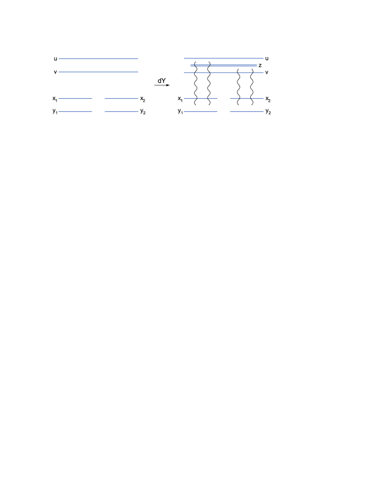
Figure 1: Dipole splitting in the target

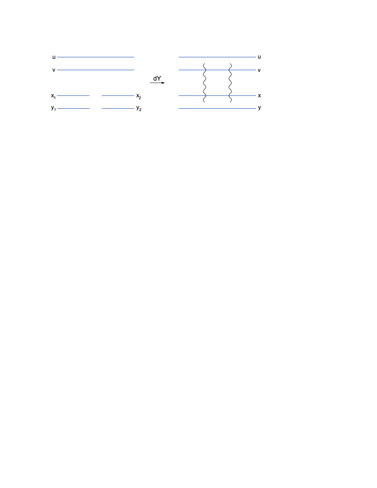
Figure 2: Dipoles (effectively) “recombining” in the projectile

Appendix A Evolution equations for a generic reaction–diffusion process

In this section we present, for completeness, the general evolution equations for a generic reaction–diffusion process with non–local vertices for splitting and merging. Particular cases of these equations have already appeared in the main body of the paper.

We consider the reaction–diffusion process $A\rightleftharpoons A+A$ in which one particle at position $x$ can split into two particles at positions $x_{1}$ and $x_{2}$ at a rate $\alpha(x|x_{1}x_{2})$, and two particles at positions $x_{1}$ and $x_{2}$ can merge into one particle at position $x$ at a rate $\beta(x_{1}x_{2}|x)$. We denote by $P_{N}(x_{1}\dots x_{N})\equiv P_{N}(X)$ the probability density to observe a system of $N$ particles at positions $x_{1},\dots,x_{N}$ at a given time $t$ (the dependence of $P_{N}$ upon $t$ is kept implicit). Due to merging and splitting, the probabilities evolve according to the following hierarchy of equations, which is usually referred to as the Master equation :

$$\partial_{t}P_{N}(X) \!=\! \sum_{i\neq j}\int_{z}\alpha(z|x_{i}x_{j})P_{N-1}(x_{1}\dots\not{x}_{i}\dots\not{x}_{j}\dots x_{N}z)-\sum_{i}\int_{z_{1},z_{2}}\alpha(x_{i}|z_{1}z_{2})P_{N}(X)$$ (A.18)

$$\!+\! \sum_{i}\int_{z_{1},z_{2}}\beta(z_{1}z_{2}|x_{i})P_{N+1}(x_{1}\dots\not{x}_{i}\dots x_{N}z_{1}z_{2})-\sum_{i\neq j}\int_{z}\beta(x_{i}x_{j}|z)P_{N}(X).$$

In writing this equation, we have also assumed the symmetry properties $\alpha(x|x_{1}x_{2})=\alpha(x|x_{2}x_{1})$ and $\beta(x_{1}x_{2}|x)=\beta(x_{2}x_{1}|x)$

Let us now derive the equation for the evolution of an observable ${\cal O}$ with an average value defined by

$$\left\langle{\cal O}\right\rangle=\sum_{N=1}^{\infty}\int d\Gamma_{N}P_{N}(x_{1}\dots x_{N}){\cal O}_{N}(x_{1}\dots x_{N}),$$

where in the integral over the phase–space one needs to count only once the configurations differing only by the order of their elements (cf. Eq. (4.5)). After some straightforward algebra, we obtain the following evolution equation for the observable

$$\partial_{t}\left\langle{\cal O}\right\rangle=\sum_{N=1}^{\infty}\frac{1}{N!}\int_{x_{i}} P_{N}(X)\left\{\sum_{i=1}^{N}\int_{z_{1},z_{2}}\alpha(x_{i}|z_{1}z_{2})\left[{\cal O}_{N+1}(x_{1}\dots\not{x}_{i}\dots x_{N}z_{1}z_{2})-{\cal O}_{N}(X)\right]\right.$$ (A.19)

$$+\left.\sum_{i\neq j}\int_{z}\beta(x_{i}x_{j}|z)\left[{\cal O}_{N-1}(x_{1}\dots\not{x}_{i}\dots\not{x}_{j}\dots x_{N}z)-{\cal O}_{N}(X)\right]\right\},$$

which encompasses Eqs. (4.8) and (4.19) of the main text.

In particular, let us derive the evolution equations for the average $k$–particle densities. The average particle number density $\left\langle n(y)\right\rangle$ is defined as in Eq. (4.9), and involves the following density operator

$$n_{N}(y|x_{1}\dots x_{N})=\sum_{i=1}^{N}\delta_{yx_{i}}.$$ (A.20)

Similarly, the $k$–particle density operator is defined as

$$n^{(k)}_{N}(y_{1}\dots y_{k}|x_{1}\dots x_{N})=\sum_{i_{1}\neq\dots\neq i_{k}}\delta_{y_{1}x_{i_{1}}}\dots\delta_{y_{k}x_{i_{k}}}.$$

Inserting the definition (A.20) into the evolution equation (A.19) gives

$$\partial_{t}\left\langle n(y)\right\rangle \!=\! \int_{z_{1},z_{2}}\alpha(z_{1}|yz_{2})\left\langle n(z_{1})\right\rangle+\alpha(z_{2}|z_{1}y)\left\langle n(z_{2})\right\rangle-\alpha(y|z_{1}z_{2})\left\langle n(y)\right\rangle$$

$$+\beta(z_{1}z_{2}|y)\left\langle n^{(2)}(z_{1}z_{2})\right\rangle-\beta(z_{1}y|z_{2})\left\langle n^{(2)}(z_{1},y)\right\rangle-\beta(yz_{2}|z_{1})\left\langle n^{(2)}(yz_{2})\right\rangle.$$

In a similar way, but after some lengthier manipulations, one ends up with the following evolution equation for the general $k$–particle density:

$$\partial_{t}\left\langle n^{(k)}(y_{1}\dots vy_{k})\right\rangle$$

$$= \int_{z_{1},z_{2}}\sum_{i=1}^{k}\alpha(z_{1}|yz_{2})\left\langle n^{(k)}(y_{1}\dots y_{i-1}z_{1}y_{i+1}\dots y_{k})\right\rangle-\beta(z_{1}y|z_{2})\left\langle n^{(k+1)}(y_{1}\dots y_{k}z_{1})\right\rangle$$

$$\phantom{\int_{z_{1}}\sum}+\alpha(z_{2}|z_{1}y)\left\langle n^{(k)}(y_{1}\dots y_{i-1}z_{2}y_{i+1}\dots y_{k})\right\rangle-\beta(yz_{2}|z_{1})\left\langle n^{(k+1)}(y_{1}\dots y_{k}z_{2})\right\rangle$$

$$\phantom{\int_{z_{1}}\sum}-\alpha(y|z_{1}z_{2})\left\langle n^{(k)}(y_{1}\dots y_{k})\right\rangle+\beta(z_{1}z_{2}|y)\left\langle n^{(k+1)}(y_{1}\dots\not{y}_{i}\dots y_{k}z_{1}z_{2})\right\rangle$$

$$+ \int_{z}\sum_{i\neq j}\alpha(z|y_{i}y_{j})\left\langle n^{(k-1)}(y_{1}\dots\not{y}_{i}\dots\not{y}_{j}\dots y_{k}z)\right\rangle-\beta(y_{i}y_{j}|z)\left\langle n^{(k)}(y_{1}\dots y_{k})\right\rangle.$$

Finally, we use the density operators to construct a scattering amplitude which includes multiple scattering to all orders. This is defined as [27]

$${\cal A}(t)=\sum_{k}\frac{1}{k\,!}\int_{x_{i}}(-)^{k+1}T^{(k)}(x_{1}\dots x_{k};t_{0})\,n^{(k)}(x_{1}\dots x_{k};t-t_{0})\vspace{-.5cm}$$ (A.23)

with $T^{(k)}$ being the scattering amplitude for a set of $k$ particles. In this expression $t_{0}$ represents an arbitrary intermediate time, but the physical quantity ${\cal A}(t)$ is of course independent of $t_{0}$ : $d{\cal A}(t)/dt_{0}=0$. From this condition together with the evolution equation for the average densities derived before, one can finally deduce a set of evolution equations for the scattering amplitudes. The general equation in this hierarchy reads:

$$\partial_{t}T^{(k)}(x_{1}\dots x_{k};t) \!=\! \sum_{i=1}^{k}\int_{z_{1},z_{2}}\alpha(x_{i}|z_{1}z_{2})\left[T^{(k)}(x_{1}\dots\not{x}_{i}\dots x_{k}z_{1};t)+T^{(k)}(x_{1}\dots\not{x}_{i}\dots x_{k}z_{2};t)\right.$$

$$\phantom{\sum_{i=1}^{k}z1z2\alpha(x_{i}|z_{1}z_{2})}\left.-T^{(k)}(x_{1}\dots x_{k};t)-T^{(k+1)}(x_{1}\dots\not{x}_{i}\dots y_{k}z_{1}z_{2};t)\right]$$

$$\!+\! \sum_{i\neq j}\int_{z_{1}}\beta(x_{i}x_{j}|z)\left[T^{(k-1)}(x_{1}\dots\not{x}_{i}\dots x_{k};t)+T^{(k-1)}(x_{1}\dots\not{x}_{j}\dots x_{k};t)\right.$$

$$\phantom{\sum_{i=1}^{k}z_{1}\alpha(x_{i}|z_{1}z_{2})}\left.-T^{(k-1)}(x_{1}\dots\not{x}_{i}\dots\not{x}_{j}\dots y_{k}z;t)-T^{(k)}(x_{1}\dots x_{k};t)\right].$$

References

- [1] E. Iancu and A.H. Mueller, Nucl. Phys. A730 (2004) 494.
- [2] A.H. Mueller and A.I. Shoshi, Nucl. Phys. B692 (2004) 175.
- [3] E. Iancu, A.H. Mueller and S. Munier, Phys. Lett. B606 (2005) 342.
- [4] E. Iancu and D.N. Triantafyllopoulos, Nucl. Phys. A756 (2005) 419.
- [5] I. Balitsky, Nucl. Phys. B463 (1996) 99; Phys. Lett. B518 (2001) 235; “High-energy QCD and Wilson lines”, arXiv:hep-ph/0101042.
- [6] J. Jalilian-Marian, A. Kovner, A. Leonidov and H. Weigert, Nucl. Phys. B504 (1997) 415; Phys. Rev. D59 (1999) 014014; J. Jalilian-Marian, A. Kovner and H. Weigert, Phys. Rev. D59 (1999) 014015; A. Kovner, J. G. Milhano and H. Weigert, Phys. Rev. D62 (2000) 114005.
- [7] E. Iancu, A. Leonidov and L. McLerran, Nucl. Phys. A692 (2001) 583; Phys. Lett. B510 (2001) 133; E. Ferreiro, E. Iancu, A. Leonidov and L. McLerran, Nucl. Phys. A703 (2002) 489.
- [8] H. Weigert, Nucl. Phys. A703 (2002) 823.
- [9] E. Iancu, D.N. Triantafyllopoulos, Phys. Lett. B610 (2005) 253.
- [10] A.H. Mueller, A.I. Shoshi, S.M.H. Wong, Nucl. Phys. B715 (2005) 440.
- [11] J.-P. Blaizot, E. Iancu, K. Itakura, D.N. Triantafyllopoulos, Phys. Lett. B615 (2005) 221.
- [12] E. Levin, M. Lublinsky, “Towards a symmetric approach to high energy evolution: generating functional with Pomeron loops”, arXiv:hep-ph/0501173.
- [13] E. Levin, “High energy amplitude in the dipole approach with Pomeron loops: asymptotic solution”, arXiv:hep-ph/0502243.
- [14] A. Kovner and M. Lublinsky, Phys. Rev. D71 (2005) 085004.
- [15] A. Kovner and M. Lublinsky, Phys. Rev. Lett. 94 (2005) 181603.
- [16] A. Kovner and M. Lublinsky, “Dense-Dilute Duality at work: dipoles of the target”, arXiv:hep-ph/0503155.
- [17] Y. Hatta, E. Iancu, L. McLerran, A. Stasto, D.N. Triantafyllopoulos, “Effective Hamiltonian for QCD Evolution at High Energy”, hep-ph/0504182, to appear in Nucl.Phys. A.
- [18] C. Marquet, A.H. Mueller, A.I. Shoshi, and S.M.H. Wong “On the Projectile-Target Duality of the Color Glass Condensate in the Dipole Picture”, arXiv:hep-ph/0505229.
- [19] Y. Hatta, E. Iancu, L. McLerran, and A. Stasto, “ Color dipoles from Bremsstrahlung in QCD evolution at high energy”, arXiv:hep-ph/0505235, to appear in Nucl. Phys. A.
- [20] I. Balitsky, “High-enegy effective action from scattering of QCD shock waves”, arXiv:hep-ph/0507237.
- [21] A. Kovner and M. Lublinsky, “More Remarks on High Energy Evolution”, arXiv:hep-ph/0510047.
- [22] A.H. Mueller, Nucl. Phys. B415 (1994) 373; A.H. Mueller, B. Patel, Nucl. Phys. B425 (1994) 471.
- [23] A.H. Mueller, Nucl. Phys. B437 (1995) 107.
- [24] E. Iancu and A.H. Mueller, Nucl. Phys. A730 (2004) 460.
-
[25]
L.N. Lipatov, Sov. J. Nucl. Phys. 23 (1976) 338;
E.A. Kuraev, L.N. Lipatov and V.S. Fadin, Zh. Eksp. Teor. Fiz 72, 3 (1977) (Sov. Phys. JETP 45 (1977) 199);
Ya.Ya. Balitsky and L.N. Lipatov, Sov. J. Nucl. Phys. 28 (1978) 822. - [26] G.P. Salam, Nucl. Phys. B449 (1995) 589; Nucl. Phys. B461 (1996) 512; A.H. Mueller, G.P. Salam, Nucl. Phys. B475 (1996) 293.
- [27] Yu.V. Kovchegov, Phys. Rev. D60 (1999), 034008; ibid. D61 (1999), 074018.
- [28] E. Levin and M. Lublinsky, Phys. Lett. B607 (2005) 131.
- [29] L. McLerran and R. Venugopalan, Phys. Rev. D49 (1994) 2233; ibid. 49 (1994) 3352; ibid. 50 (1994) 2225.
-
[30]
E. Iancu, A. Leonidov and L. McLerran, “The Colour Glass Condensate: An
Introduction”, arXiv:hep-ph/0202270. Published in QCD Perspectives on
Hot and Dense Matter, Eds. J.-P. Blaizot and E. Iancu, NATO Science Series,
Kluwer, 2002;
E. Iancu and R. Venugopalan, “The Color Glass Condensate and High Energy Scattering in QCD”, arXiv:hep-ph/0303204. Published in Quark-Gluon Plasma 3, Eds. R.C. Hwa and X.-N. Wang, World Scientific, 2003;
H. Weigert, “Evolution at small : The Color Glass Condensate”, arXiv:hep-ph/0501087. - [31] J.-P. Blaizot, E. Iancu and H. Weigert, Nucl. Phys. A713 (2003) 441.
- [32] K. Rummukainen and H. Weigert, Nucl. Phys. A739 (2004) 183.
- [33] J. Bartels and M. Wüsthoff, Z. Phys. C66 (1995) 157.
- [34] M. Braun and G.P. Vacca, Eur. Phys. J. C6 (1999) 147; M. Braun, Phys. Lett. B483 (2000) 115.
- [35] R.A. Janik, Phys. Lett. B604 (2004) 192.
- [36] C.W. Gardiner, Handbook of Stochastic Methods, Springer, Berlin, 2004.
- [37] W. Van Saarloos, Phys. Rep. 386 (2003) 29; D. Panja, Phys. Rep. 393 (2004) 87.
- [38] S. Munier and R. Peschanski, Phys. Rev. Lett. 91 (2003) 232001; Phys. Rev. D69 (2004) 034008; ibid. D70 (2004) 077503.
- [39] A.M. Stasto, K. Golec-Biernat and J. Kwiecinski, Phys. Rev. Lett. 86 (2001) 596.
- [40] E. Iancu, K. Itakura, and L. McLerran, Nucl. Phys. A708 (2002) 327.
- [41] A.H. Mueller and D.N. Triantafyllopoulos, Nucl. Phys. B640 (2002) 331.
- [42] D.N. Triantafyllopoulos, Nucl. Phys. B648 (2003) 293.
- [43] Yu.V. Kovchegov, “Inclusive Gluon Production In High Energy Onium-Onium Scattering”, arXiv:hep-ph/0508276.
- [44] E. Iancu and L. McLerran, Phys. Lett. B510 (2001) 145.
- [45] A. H. Mueller, Nucl. Phys. B643 (2002) 501.
- [46] E. Levin and M. Lublinsky, Nucl. Phys. A730 (2004) 191.
- [47] G. Soyez, Phys. Rev. D72 (2005) 016007.
- [48] R. Enberg, K. Golec–Biernat, S. Munier, “The high energy asymptotics of scattering processes in QCD”, arXiv:hep-ph/0505101.
- [49] Y. Hatta, E. Iancu, K. Itakura and L. McLerran, Nucl. Phys. A760 (2005) 172.