Developments in perturbative QCD

Abstract

A brief review of key recent developments and ongoing projects in perturbative QCD theory, with emphasis on conceptual advances that have the potential for impact on LHC studies. Topics covered include: twistors and new recursive calculational techniques; automation of one-loop predictions; developments concerning NNLO calculations; the status of Monte Carlo event generators and progress in matching to fixed order; analytical resummation including the push to NNLL, automation and gap between jets processes; and progress in the understanding of saturation at small $x$.

1 Introduction

A significant part of today’s research in QCD aims to provide tools to help better constrain the standard model and find what may lie beyond it. For example one wishes to determine, as accurately as possible, the fundamentals of the QCD and electroweak theories, such as $\alpha_{s}$, quark masses, and the elements of the CKM matrix. One also needs precise information about ‘pseudo-fundamentals,’ quantities such as parton distribution functions (PDFs) that could be predicted if we knew how to solve non-perturbative QCD, but which currently must be deduced from experimental data. Finally, one puts this information together to predict the QCD aspects of both backgrounds and signals at high energy colliders, particularly at the Tevatron and LHC, to help maximise the chance of discovering and understanding any new physics.

Other facets of QCD research seek to extend the boundaries of our knowledge of QCD itself. The underlying Yang-Mills field theory is rich in its own right, and unexpected new perturbative structures have emerged in the past two years from considerations of string theory. In the high-energy limit of QCD it is believed that a new state appears, the widely studied colour glass condensate, which still remains to be well understood. And perhaps the most challenging problem of QCD is that of how to relate the partonic and hadronic degrees of freedom.

Given the practical importance of QCD for the upcoming LHC programme, this talk will concentrate on results (mostly since the 2003 Lepton-Photon symposium) that bring us closer to the well-defined goals mentioned in the first paragraph. Some of the more explorative aspects will also be encountered as we go along, and one should remember that there is constant cross-talk between the two. For example: improved understanding of field theory helps us make better predictions for multi-jet events, which are important backgrounds to new physics; and by comparing data to accurate perturbative predictions one can attempt to isolate and better understand the parton-hadron interface.

The first part of this writeup will be devoted to results at fixed order. At tree level we will examine new calculational methods that are much more efficient than Feynman graphs; we will then consider NLO and NNLO calculations and look at the issues that arise in going from the Feynman graphs to useful predictions.

One of the main uses of fixed-order order predictions is for understanding rare events, those with extra jets. In the second part of the writeup we shall instead turn to resummations, which help us understand the properties of typical events.

Throughout, the emphasis will be on the conceptual advances rather than the detailed phenomenology. Due to lack of space, some active current topics will not be covered, in particular exclusive QCD. Others are discussed elsewhere in these proceedings.[1]

2 Fixed-order calculations

2.1 Tree-level amplitudes and twistors

Many searches for new physics involve signatures with a large number of final-state jets. Even for as basic a process as $t\bar{t}$ production, the most common decay channel (branching ratio of 46%), $t\bar{t}\to b\bar{b}W^{+}W^{-}\to b\bar{b}qq\bar{q}\bar{q}$ involves 6 final-state jets, to which there are large QCD multi-jet backgrounds.[2] And at the LHC, with $10\,\mathrm{fb}^{-1}$ (1 year) of data, one expects of the order of 2000 events with 8 or more jets[3] ($p_{t}(\mathsf{jet})>60\,\mathrm{GeV}$, $\theta_{ij}>30\deg$, $|y_{i}|<3$).

For configurations with such large numbers of jets, even tree-level calculations become a challenge — for instance $gg\to 8g$ involves 10525900 Feynman diagrams (see ref.[4]). In the 1980’s, techniques were developed to reduce the complexity of such calculations.[5] Among them colour decomposition,[6] where one separates the colour and Lorentz structure of the amplitude,

$${\cal A}^{\mathsf{tree}}(1,2,\ldots,n)=g^{n-2}\sum_{perms}\\ \underbrace{\mathsf{Tr}(T_{1}T_{2}\ldots T_{n})}_{\textsf{colour struct.}}\underbrace{A^{\mathsf{tree}}(1,2,\ldots,n)}_{\textsf{colour ordered amp.}}\,;$$ (1)

the use[7] of spinor products $\langle ij\rangle\equiv\langle i^{-}|j^{+}\rangle=\overline{u_{-}(k_{i})}u_{+}(k_{j})$ and $[ij]=\langle i^{+}|j^{-}\rangle$ as the key building blocks for writing amplitudes; and the discovery[8] and subsequent proof[9] of simple expressions for the subset of amplitudes involving the maximal number of same-helicity spinors (maximum helicity violating or MHV amplitudes), i.e. $n-2$ positive helicity spinors for an $n$-gluon amplitude:

$$A^{\mathrm{tree}}(--++\ldots)=\frac{i\langle 12\rangle^{4}}{\langle 12\rangle\langle 23\rangle\ldots\langle n1\rangle}\,.$$ (2)

Ref.[9] also provided a computationally efficient recursion relation for calculating amplitudes with arbitrary numbers of legs, and with these and further techniques,[10] numerous programs (e.g. MadEvent,[11] ALPGEN,[12] HELAC/PHEGAS,[13] CompHEP,[14] GRACE,[15] Amegic[16]) are able to provide results for processes with up to 10 legs.

The past two years have seen substantial unexpected progress in the understanding of multi-leg tree-level processes. It was initiated by the observation (first made by Nair[17]) that helicity amplitudes have a particularly simple form in ‘twistor’ space, a space where a Fourier transform has been carried out with respect to just positive helicity spinors. In twistor space a duality appears[18] between the weakly-coupled regimes of a topological string theory and ${\cal N}=4$ SUSY Yang-Mills. This has led to the postulation, by Cachazo, Svrcek and Witten (CSW),[19] of rules for deriving non-MHV ${\cal N}=4$ SUSY amplitudes from MHV ones, illustrated in fig. 1. For purely gluonic amplitudes the results are identical to plain QCD,[20] because tree level SUSY amplitudes whose external legs are gluons have only gluonic propagators.

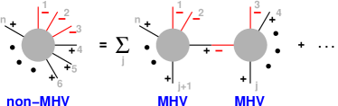
Figure 1: Graphical illustration of the CSW rules: by joining together two MHV amplitudes with an off-shell scalar propagator one obtains an amplitude with an extra negative helicity (NMHV).

Recently a perhaps even more powerful set of recursion relations was proposed by Britto, Cachazo and Feng (BCF),[21] which allows one to build a general $n$-leg diagram by joining together pairs of on-shell sub-diagrams. This is made possible by continuing a pair of reference momenta into the complex plane. The proof[22] of these relations (and subsequently also of the CSW rules[23]) is remarkably simple, based just on the planar nature of colour-ordered tree diagrams, their analyticity structure, and the asymptotic behaviour of known MHV amplitudes.

The discovery of the CSW and BCF recursion relations has spurred intense activity, about 150 articles citing the original papers[18, 19] having appeared in the 18 months following their publication. Questions addressed include the derivation of simple expressions for specific amplitudes,[24] the search for computationally efficient recursive formulations,[25] extensions to processes with fermions and gluinos,[26] Higgs bosons,[27] electroweak bosons,[28] gravity,[29] and the study of multi-gluon collinear limits.[30] This list is necessarily incomplete and further references can be found in a recent review[31] as well as below, when we discuss applications to loop amplitudes.

2.2 One-loop amplitudes

For quantitatively reliable predictions of a given process it is necessary for it to have been calculated to next-to-leading order (NLO). A wide variety of NLO calculations exists, usually in the form of publicly available programs,[32] that allow one to make predictions for arbitrary observables within a given process. The broadest of these programs are the MCFM,[33] NLOJET[34] and PHOX[35] families.

For a $2\to n$ process the NLO calculation involves the $2\to n+1$ tree-level diagram, the $2\to n$ 1-loop diagram, and some method for combining the tree-level matrix element with the loop contributions, so as to cancel the infrared and collinear divergences present in both with opposite signs. We have seen above that tree-level calculations are well understood, and dipole subtraction[36] provides a general prescription for combining them with the corrresponding 1-loop contributions. The bottleneck in such calculations remains the determination of the 1-loop contribution. Currently, $2\to 3$ processes are feasible, though still difficult, while as yet no full $2\to 4$ 1-loop QCD calculation has been completed.

In view of the difficulty of these loop calculations, a welcome development has been the compilation, by theorists and experimenters at the Les Houches 2005 workshop, Physics at TeV Colliders,[37] of a realistic prioritised wish-list of processes. Among the most interesting remaining $2\to 3$ processes one has $pp\to WW+\mathrm{jet}$, $pp\to VVV$ ($V=W$ or $Z$) and $pp\to H+2\,\mathrm{jets}$. The latter can be considered a ‘background’ to Higgs production via vector boson fusion, insofar as the isolation of the vector-boson fusion channel for Higgs production would allow relatively accurate measurements of the Higgs couplings.[38] A number of $2\to 4$ processes are listed as backgrounds to $t\bar{t}H$ production ($pp\to t\bar{t}q\bar{q},t\bar{t}b\bar{b}$), $WW\to H\to WW$ or to general new physics ($pp\to V+3\,\mathrm{jets}$) or specifically SUSY ($pp\to VVV+\,\mathrm{jet}$).

Two broad classes of techniques have been used in the past for 1-loop calculations: those based directly on the evaluation of the Feynman diagrams (sometimes for the 1-loop-tree interference[39]) and those based on unitarity techniques to sew together tree diagrams (see the review[40]). Both approaches are still being actively pursued.

Today’s direct evaluations of 1-loop contributions have, as a starting point, the automated generation of the full set of Feynman diagrams, using tools such as QGRAF[41] and FeynArts.[42] The results can be expressed in terms of sums of products of group-theoretic (e.g. colour) factors and tensor one-loop integrals, such as

$$I_{n;\mu_{1}..\mu_{i}}=\int d^{4+2\epsilon}\ell\frac{\ell_{\mu_{1}}\ldots\ell_{\mu_{i}}}{(\ell+k_{1})^{2}\ldots(\ell+k_{n})^{2}}$$ (3)

Reduction procedures exist (e.g.[43, 44]) that can be applied recursively so as to express the $I_{n;\mu_{1}..\mu_{i}}$ in terms of known scalar integrals. Such techniques form the basis of recent proposals for automating the evaluation of the integrals, where the recursion relations are solved by a combination of analytical and numerical methods,[45] or purely numerically,[46, 47, 48] in some cases with special care as regards divergences that appear in the coefficients of individual terms of the recursion relation but vanish in the sum.[47, 49] Results from these approaches include a new compact form for $gg\to g\gamma\gamma$ at 1 loop[50] and the 1-loop contribution to the ‘priority’ $pp\to H+2\,\mathrm{jets}$ process.[51] Related automated approaches have also been developed in the context of electroweak calculations,[52] where recently a first $2\to 4$ 1-loop result ($e^{+}e^{-}\to 4$ fermions) was obtained.[53]

Another approach[54] proposes subtraction terms for arbitrary 1-loop graphs, such that the remaining part of the loop integral can carried out numerically in 4 dimensions. The subtraction terms themselves can be integrated analytically for the sum over graphs and reproduce all infrared, collinear and ultraviolet divergences.

The above methods are all subject to the problem of the rapidly increasing number of graphs for multi-leg processes. On the other hand, procedures based on ‘sewing’ together tree graphs to obtain loop graphs[40] (cut constructibility approach) can potentially benefit from the simplifications that emerge from twistor developments for tree graphs. This works best for ${\cal N}=4$ SUSY QCD, where cancellations between scalars, fermions and vector particles makes the ‘sewing’ procedure simplest and for example all gluonic (and some scalar and gluino) NMHV 1-loop helicity amplitudes are now known;[55] also, conjectures for ${\cal N}=4$ SUSY $n$-leg MHV planar graphs, at any number of loops, based on 4-gluon two and three-loop calculations,[56] have now been explicitly verified for 5 and 6 gluon two-loop amplitudes.[57] For ${\cal N}=1$ SUSY QCD, known results for all MHV amplitudes[58] have been reproduced[59] and new results exist for some all-$n$ NMHV graphs[60] as well as full results for 6 gluons.[61] For plain QCD, progress has been slower, though all finite 1-loop graphs ($++++\ldots$, $-+++\ldots$) were recently presented[62] and understanding has also been achieved for divergent graphs,[63] including the full result for all 1-loop $(--+++\ldots)$ MHV graphs.[64] The prospects for the twistor-inspired approach are promising and one can hope that it will soon become practically competitive with the direct evaluation methods.

2.3 NNLO jet calculations

NNLO predictions are of interest for many reasons: in those processes where the perturbative series has good convergence they can help bring perturbative QCD predictions to the percent accuracy level. In cases where there are signs of poor convergence at NLO they will hopefully improve the robustness of predictions and, in all cases, give indications of the reliability of the series expansion. Finally they may provide insight in the discussion of the relative importance of hadronisation and higher-order perturbative corrections.[65, 66, 67]

So far, NNLO predictions are available mostly only for processes with 3 external legs, such as the total cross section for $Z\to\mathrm{hadrons}$ or the inclusive $pp\to W,Z$[68, 69, 70] or Higgs[69, 71, 72] cross sections. A full list is given in table 1 of Stirling’s ICHEP writeup.[73]

Most current effort is being directed to the $e^{+}e^{-}\to 3\,\mathrm{jets}$ process, where NLO corrections are often large, and where one is free of complications from incoming coloured particles. The ingredients that are needed are the squared 5-parton tree level ($M_{5}$) and 3-parton 1-loop ($M_{3a}$) amplitudes, and the interference between 4-parton tree and 1-loop ($M_{4}$), and between 3-parton tree and 2-loop amplitudes ($M_{3b}$), all of which are now known (for references see introduction of[74]). A full NNLO prediction adds the integrals over phase-space of these contributions, multiplied by some jet-observable function $J$ that depends on the momenta $p_{i}$

$$J_{NNLO}=\int d^{D}\!\Phi_{5}M_{5}J(p_{1..5})\,+\\ \int d^{D}\!\Phi_{4}M_{4}J(p_{1..4})+\int d^{D}\!\Phi_{3}(M_{3a+b})J(p_{1..3})\,.$$

Each of the terms is infrared and collinear (IRC) divergent, because of the phase space integration ($M_{4,5}$) and/or the loop integral ($M_{3,4}$). The current bottleneck for such calculations is in cancelling these divergences for an arbitrary (IRC safe) $J$.

A standard approach at NLO is to introduce subtraction terms (e.g. in the dipole[36] formalism), schematically,

$$J_{NLO}^{4-jet}=\int d^{D}\!\Phi_{5}(M_{5}J(p_{1..5})-S_{5}J(\tilde{p}_{1..4}))\\ +\int d^{D}\!\Phi_{4}(M_{4}J(p_{1..4})+S_{4}J(p_{1..4}))$$

such that each integral is separately finite and that, alone, the $S_{5}$ and $S_{4}$ terms integrate to equal and opposite divergent contributions (they both multiply the same 4-parton jet function $J(p_{1..4})$ and the $\tilde{p}_{1..4}$ are a specifically designed function of the $p_{1..5}$). At NNLO a similar method can be envisaged, and considerable work has gone towards developing a general formalism.[75, 76, 77, 78, 79, 74]

An alternative approach, sector decomposition,[80, 81, 82, 83] introduces special distributions $f_{-i}$ (involving plus-functions, like those in splitting functions), which isolate the $\epsilon^{-i}$ divergent piece of a given integral ($\epsilon=(D-4)/2$),

$$\int d^{D}\!\Phi_{5}M_{5}J(p_{1..5})=\frac{1}{\epsilon^{4}}\!\!\int d^{4}\!\Phi_{5}f_{-4}M_{5}J(p_{1..5})\\ +\frac{1}{\epsilon^{3}}\!\!\int d^{4}\!\Phi_{5}f_{-3}M_{5}J(p_{1..5})+\ldots\,,$$

where the integration is performed in transformed variables that simplify the separation of divergences. In such an approach one thus obtains separate results for each power of $\epsilon$ in both real and virtual terms, making it easy to combine them.

A useful testing ground for a number of these approaches has been $e^{+}e^{-}\to 2\,\mathrm{jets}$.[83, 84, 78] Fundamentally new results are the differential distributions for $W,Z,H$ production[85] in the sector-decomposition approach and the $(\alpha_{s}C_{F}/2\pi)^{3}$ contribution to $\langle 1-\mathrm{Thrust}\rangle$ in $e^{+}e^{-}\to 3\,\mathrm{jets}$, $-20.4\pm 4$, in the ‘antenna’ subtraction approach.[74]

2.4 NNLO splitting functions

The landmark calculation of 2004 was probably that of the NNLO splitting functions by Moch, Vermaseren and Vogt[86] (MVV). These are important for accurate DGLAP evolution of the parton distributions, as extracted from fixed target, HERA and Tevatron data, up to LHC scales.

The results for the splitting functions take about 15 pages to express, though the authors have also provided compact approximations for practical use. These are gradually being adopted in NNLO fits.[87, 88] Mostly the NNLO splitting functions are quite similar to the estimates obtained a few years ago[89] based on a subset of the moments and known asymptotic limits. In particular it remains true that the NNLO corrections are in general small, both compared to NLO and in absolute terms. The worst region is that of small $x$ for the singlet distributions, shown in fig. 2, where the NLO corrections were large and there is a significant NNLO modification as well. Studies of small-$x$ resummation suggest that further high-order effects should be modest,[90, 91] though so far only the gluon sector has been studied in detail.

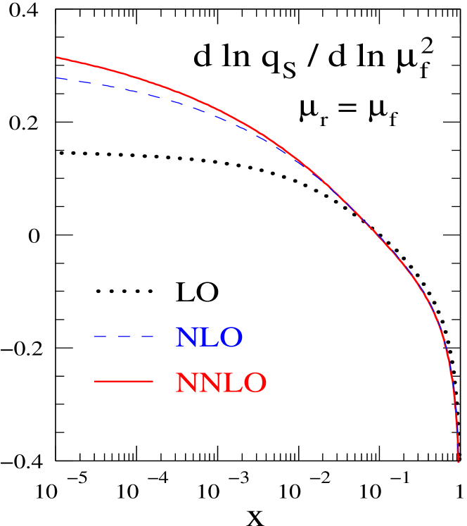
Figure 2: Impact[86] of NNLO DGLAP corrections on the derivative of a toy singlet quark distribution $q_{S}=\sum_{i}(q_{i}+\bar{q}_{i})$.

Another potentially dangerous region is that of large $x$: the splitting functions converge well, but the coefficient functions have $[\alpha_{s}^{n}\ln^{2n-1}(1-x)]/(1-x)$ enhancements. There are suggestions that the all-order inclusion of these enhancements via a threshold resummation may help improve the accuracy of PDF determinations.[92] Fresh results from the MVV group,[93] for the third order electromagnetic coefficient functions, quark and gluon form factors, and new threshold resummation coefficients should provide the necessary elements for yet higher accuracy at large $x$. Together with the large-$x$ part of the NNLO splitting functions these have been used as inputs to the N³LO soft-collinear enhanced terms for the Drell-Yan and Higgs cross sections.[94, 95]

Finally, as splitting-function calculations approach accuracies the $1\%$ level, one should consider also the relevance of QED corrections.[87, 96]

2.5 Other accuracy-related issues

In view of the efforts being devoted to improving the accuracy of theoretical predictions, it is disheartening to discover that there are still situations where accuracy is needlessly squandered through incorrect data-theory comparisons. This is the case for the inclusive jet cross sections in the cone algorithm at the Tevatron, where a parameter $R_{sep}=1.3$ is introduced in the cone algorithm used for the NLO calculation (see e.g.[97]), but not in the cone algorithm applied to the data. $R_{sep}$ is the multiple of the cone radius beyond which a pair of partons is not recombined. It dates to early theoretical work[98] on NLO corrections to the cone algorithm in hadron collisions, when there was no public information on the exact jet algorithm used by the experiments: $R_{sep}$ was introduced to parametrise that ignorance.

The use of $R_{sep}$ in just the theory introduces a spurious NLO correction (at the $5-10\%$ level[98]), meaning that the data-theory comparisons are only good to LO. The size of the discrepancy is comparable to the NLO theory uncertainty. As this is smaller than experimental errors, for now the practical impact is limited. However, as accuracies improve it is essential that theory-experiment comparisons be done consistently, be it with properly used cone algorithms[99] or with the (more straightforward and powerful) $k_{t}$ algorithm,[100] which is finally starting to be investigated.[101]

An accuracy issue that is easily overlooked when discussing QCD developments is the non-negligible impact of electroweak effects at large scales. The subject has mostly been investigated for leptonic initial and final states at a linear collider (ILC). The dominant contributions go as $\alpha_{EW}\ln^{2}P_{t}/M_{W}$. Since the LHC can reach transverse momenta ($P_{t}$) an order of magnitude larger than the ILC the electroweak effects are very considerably enhanced at the LHC, being up to $30-40\%$.[102, 103] Among the issues still to be understood in such calculations (related to the cancellation of real and virtual corrections) is the question of whether experiments will include events with $W$ and $Z$’s as part of their normal QCD event sample, or whether instead such events will be treated separately.

3 All-order calculations

All-order calculations in QCD are based on the resummation of logarithmically dominant contributions at each order. Such calculations are necessary if one is to investigate the properties of typical events, for which each extra power of $\alpha_{s}$ is accompanied by large soft and collinear logarithms.

The two main ways of obtaining all-order resummed predictions are with exclusive Monte Carlo event generators, and with analytical resummations. The former provide moderately accurate (leading log (LL) and some parts of NLL) predictions very flexibly for a wide variety of processes, with hadronisation models included. The latter are able to provide the highest accuracy (at parton level), but usually need to be carried out by hand (painfully) for each new observable and/or process. All-order calculations are also used in small-$x$ and saturation physics, which will be discussed briefly at the end of this section.

3.1 Monte Carlo event generators (MC)

Various issues are present in current work on event generators — the switch from Fortran to C++; improvements in the showering algorithms and the modelling of the underlying event; and the inclusion of information from fixed-order calculations.

The motivation for moving to C++ is the need for a more modern and structured programming language than Fortran 77. C++ is then a natural choice, in view both of its flexibility and its widespread use in the experimental community.

Originally it was intended that Herwig[104], Pythia[105] and Ariadne/LDC[106, 107] should all make use of a general C++ event generator framework known as ThePEG.[108] Herwig++,[109] based on ThePEG, was recently released for $e^{+}e^{-}$ and work is in progress for a hadron-hadron version. Pythia 7 was supposed to have been the Pythia successor based on the ThePEG, however instead a standalone C++ generator Pythia 8 is now being developed,[110] perhaps to be interfaced to ThePEG later on. Another independent C++ event generator has also recently become available, SHERPA,[111] whose showering and hadronisation algorithms are largely based on those of Pythia, and which is already functional for hadron collisions.

In both the Pythia and Herwig ‘camps’ there have been developments on new showering algorithms. Herwig++ incorporates an improved angular-ordered shower[112] in which the ‘unpopulated’ phase space regions have been shrunk. Pythia 6.3 has a new parton shower[113] based on transverse momentum ordering (i.e. somewhat like Ariadne) which provides an improved description of $e^{+}e^{-}$ event-shape data and facilitates the modelling of multiple interactions in hadron collisions. Separately, investigations of alternatives to standard leading-log backward evolution algorithms for initial-state showers are also being pursued.[114, 115]

3.2 Matching MC & fixed order

Event generators reproduce the emission patterns for soft and collinear gluons and also incorporate good models of the transition to hadrons. They are less able to deal with multiple hard emissions, which, as discussed above, are important in many new particle searches. There is therefore a need to combine event generators with fixed-order calculations.

The main approach for this is the CKKW[116] proposal. Events are generated based on the $n$-parton tree matrix elements (for various $n$), keeping an event only if its $n$ partons are sufficiently well separated to be considered as individual jets (according to some threshold jet-distance measure, based e.g. on relative $k_{t}$). Each event is then assigned a ‘best-guess’ branching history, using which it can be reweighted with appropriate Sudakov form factors (to provide virtual corrections) and running couplings. The normal parton showering is then added on to each event at scales below the threshold jet-distance measure. Over the past two years this method has become widely adopted and is available in all major generators.[117]

As well as seeking to describe more jets it is also important to increase the accuracy of event generators for limited number of jets, by including NLO corrections. Here too there is one method that has so far dominated practical uses, known as MC@NLO.[118] Very roughly, it takes the standard MC and modifies it according to

$$\mathrm{MC}\to\mathrm{MC}(1+\mathrm{NLO}-\mathrm{NLO}_{\mathrm{MC}})\,,$$ (4)

where $\mathrm{NLO}_{\mathrm{MC}}$ represents the effective NLO corrections present by default in the MC. Since the MC usually has the correct soft and collinear divergences, the combination $\mathrm{NLO}-\mathrm{NLO}_{\mathrm{MC}}$ should be finite. Eq. (4) is therefore a well-behaved way of introducing exactly the correction needed to guarantee NLO correctness. A prediction from MC@NLO for $b$-production,[119] figure 3, is compared to data and a purely analytical approach,[120] and one notes the good agreement between all three.

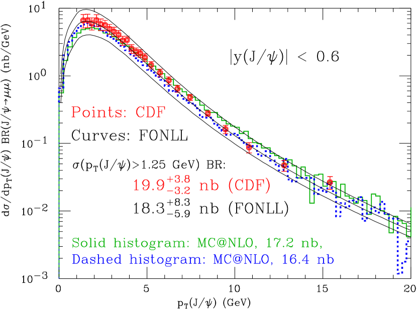
Figure 3: Spectrum for $b$-production ($\to J/\Psi$) compared to MC@NLO and an analytical prediction.[120]

A bottleneck in widespread implementation of the MC@NLO approach is the need to know $\mathrm{NLO}_{\mathrm{MC}}$, which is different for each generator, and even process. Furthermore MC@NLO so far guarantees NLO correctness only for a fixed number of jets — e.g. it can provide NLO corrections to $W$ production, but then $W+1\,\mathrm{jet}$ is only provided to LO. An approach to alleviate both these problems proposes[121] to combine, for example, $W$, $W+1\,\mathrm{jet}$, $W+2\,\mathrm{jets}$, etc. with a procedure akin to CKKW. It seeks to alleviate the problem of needing to calculate $\mathrm{NLO}_{\mathrm{MC}}$ as follows: when considering $W+m\,\mathrm{jets}$ the $(m+1)^{\mathrm{th}}$ emission (that needed for NLO accuracy) is generated not by the main MC, but by a separate mini well-controlled generator, designed specifically for that purpose and whose NLO expansion is easily calculated (as is then the analogue of eq.(4)). The only implementation of this so far (actually of an earlier, related formalism[122]) has been for $e^{+}e^{-}$.[123]

3.3 Analytical resummations

It is in the context of analytical resummations that one can envisage the highest resummation accuracies, as well as the simplest matching to fixed order calculations. Rather than directly calculating the distribution $d\sigma(V)/dV$ of an observable $V$, one often considers some integral transform $F(\nu)$ of the distribution so as to reduce $F(\nu)$ to the form

$$\ln F(\nu)=\sum_{n}(\underbrace{\alpha_{s}^{n}L^{n+1}}_{\mathrm{LL}}+\underbrace{\alpha_{s}^{n}L^{n}}_{\mathrm{NLL}}+\ldots)\,,$$ (5)

with $L=\ln\nu$.

Much of the information for certain N³LL threshold resummations was recently provided by the MVV group.[93] The highest accuracy for full phenomenological distributions is for the recently calculated Higgs transverse momentum spectrum[124] at the LHC and the related[125] energy-energy-correlation (EEC) in $e^{+}e^{-}$,[126] both of which have also been matched to NLO fixed order.

Boson transverse momentum spectra and the EEC are among the simplest observables to resum. For more general observables and processes, such as event shapes or multi-jet events, the highest accuracy obtained so far has been NLL, and the calculations are both tedious and error-prone. This has prompted work on understanding general features of resummation. One line of research[127] examines the problem of so-called ‘factorisable’ observables, for an arbitrary process. This extends the understanding of large-angle soft colour evolution logarithms, whose resummation was originally pioneered for 4-jet processes by the Stony Brook group,[128, 129] in which unexplained hidden symmetries were recently discovered,[130, 131] notably between kinematic and colour variables.

Separately, the question of how to treat general observables has led to a procedure for automating resummations for a large class of event-shape-like observables.[132] It avoids the need to find an integral transform that factorises the observable and introduces a new concept, recursive infrared and collinear safety, which is a sufficient condition for the exponentiated form eq. (5) to hold. Its main application so far has been to hadron-collider dijet event shapes,[133] (see also[134]) which provide opportunities for experimental investigation of soft-colour evolution and of hadronisation and the underlying event at the Tevatron and LHC.

The above resummations apply to ‘global’ observables, those sensitive to radiation everywhere in an event. For non-global observables, such as gap probabilities[135] or properties of individual jets,[136, 137] a new class of enhanced term appears, non-global logarithms $\alpha_{s}^{n}L^{n}$ (NGL), fig. 4. Their resummation has so far only been possible in the large-$N_{C}$ limit,[136, 138] though the observation of structure related to BFKL evolution,[139] has inspired proposals for going to finite $N_{C}$.[140]

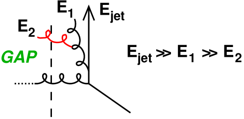
Figure 4: Diagram giving NGL: to calculate the probability of there being no emission into the gap, one should resum a large-angle energy-ordered cascade of emissions rather than just direct emission from the original hard partons.

Non-global and soft colour resummations (in non-inclusive form[129]) come together when calculating the probability of a gap between a pair of jets at the Tevatron/LHC, relevant as a background to the $W$ fusion process for Higgs production.[141] Recently it has been pointed out that contributions that are subleading in $1/N_{C}^{2}$ play an important role for large gaps,[142] and also that there are considerable subtleties when using a $k_{t}$ jet algorithm to to define the gap.[143]

3.4 Small $x$ and saturation

The rise of the gluon at small $x$, as predicted by BFKL,[144] leads eventually to such high gluon densities that a ‘saturation’ phenomenon should at some point set in. Usually one discusses this in terms of a saturation scale, $Q^{2}_{s}(x)$, below (above) which the gluon distribution is (un)saturated. From HERA data, it is believed that at $x=x_{0}\simeq 10^{-4}-10^{-5}$, $Q_{s}$ is of order $1\,\mathrm{GeV}$ and that it grows as $Q^{2}_{s}(x)=(x/x_{0})^{-\lambda}\,\mathrm{GeV}^{2}$ with $\lambda\simeq 0.3$.[145] $Q_{s}$ may be of relevance to the LHC because the typical transverse scale $E_{m}$ of minimum bias minijets should satisfy the relation $Q_{s}^{2}(s/E_{m}^{2})\sim E_{m}^{2}$, whose solution gives $E_{m}\sim(sx_{0})^{\frac{\lambda}{2+\lambda}}\,\mathrm{GeV}^{\frac{2-\lambda}{2+\lambda}}\simeq 2.7-3.6\,\mathrm{GeV}$, or if one doesn’t trust the normalisation, a factor 1.7 relative to the Tevatron. The exact phenomenology is however delicate.[146, 147]

The theoretical study of the saturation scale has seen intense activity these past 18 months, spurred by two observations. Firstly it was pointed out[148] that the Balitsky-Kovchegov (BK) equation, often used to describe the onset of saturation and the evolution $d\ln Q^{2}_{s}/d\ln x$, is in the same universality class as the Fisher Kolmogorov Petrovsky Piscounov (FKPP) reaction-diffusion equation, much studied in statistical physics[149] and whose travelling wave solutions relate to the evolution of the saturation scale. Secondly, large corrections were discovered[150] when going beyond the BK mean-field approximation: to LO, $\lambda_{BK}\propto\alpha_{s}$, while the non mean-field corrections go as $\alpha_{s}/\ln^{2}\alpha_{s}^{2}$. Such corrections turn out to be a familiar phenomenon in stochastic versions of the FKPP equation, with $\alpha_{s}^{2}$ in QCD playing the role of the minimum particle density in reaction-diffusion systems with a finite number of particles.[151] The stochastic corrections also lead to a large event-by-event dispersion in the saturation scale.

These stochastic studies are mostly based on educated guesses as to the form of the small-$x$ evolution beyond the mean-field approximation. There has also been extensive work on finding the full equation that replaces BK beyond the mean-field approximation, a number of new formulations having been proposed.[152, 153, 154, 155] It will be interesting to examine how their solutions compare to the statistical physics related approaches.

4 Concluding remarks

Of the topics covered here, the one that has been the liveliest in the past year is that of ‘twistors’. Its full impact cannot yet be gauged, but the dynamic interaction between the QCD and string-theory communities on this subject will hopefully bring further important advances.

More generally one can ask if QCD is on track for the LHC. Progress over the past years, both calculationally and phenomenologically (e.g. PDF fitting) has been steady. Remaining difficulties, for example in high (NNLO) and moderate (NLO) accuracy calculations are substantial, however the considerable number of novel ideas currently being discussed encourages one to believe that significant further advances will have been made by the time LHC turns on.

DISCUSSION

Bennie Ward

(Baylor University):
To what extent are the deduced MHV rules using twistors now proven?

Gavin Salam:

an outline of a field-theoretic proof for the MHV (CSW) rules was given in the same article[22] as the proof of the BCF rules. Recently (after the Lepton Photon Symposium) a more detailed version of the proof has appeared.[23]

References

- [1] I. Stewart, these proceedings; G. Ingelman, these proceedings.
- [2] A. Juste, these proceedings.
- [3] P. D. Draggiotis, R. H. P. Kleiss and C. G. Papadopoulos, Eur. Phys. J. C 24, 447 (2002).
- [4] E. W. N. Glover, ‘Precision Phenomenology and Collider Physics’, talk given at Computer Algebra and Particle Physics workshop, DESY Zeuthen, April 2005.
- [5] Reviewed in L. J. Dixon, hep-ph/9601359.
- [6] F. A. Berends and W. Giele, Nucl. Phys. B 294, 700 (1987); M. L. Mangano, S. J. Parke and Z. Xu, Nucl. Phys. B 298 653 (1988); M. L. Mangano, Nucl. Phys. B 309, 461 (1988).
- [7] J. F. Gunion and Z. Kunszt, Phys. Lett. B 161 333 (1985). R. Kleiss and W. J. Stirling, Nucl. Phys. B 262, 235 (1985).
- [8] S. J. Parke and T. R. Taylor, Phys. Rev. Lett. 56, 2459 (1986).
- [9] F. A. Berends and W. T. Giele, Nucl. Phys. B 306, 759 (1988).
- [10] F. Caravaglios and M. Moretti, Phys. Lett. B 358, 332 (1995).
- [11] F. Maltoni and T. Stelzer, JHEP 0302, 027 (2003).
- [12] M. L. Mangano et al., JHEP 0307, 001 (2003).
- [13] A. Kanaki and C. G. Papadopoulos, hep-ph/0012004.
- [14] A. Pukhov et al., hep-ph/9908288.
- [15] F. Yuasa et al., Prog. Theor. Phys. Suppl. 138, 18 (2000).
- [16] F. Krauss, R. Kuhn and G. Soff, JHEP 0202, 044 (2002)[hep-ph/0109036].
- [17] V. P. Nair, Phys. Lett. B 214, 215 (1988).
- [18] E. Witten, Commun. Math. Phys. 252, 189 (2004); R. Roiban, M. Spradlin and A. Volovich, JHEP 0404, 012 (2004).
- [19] F. Cachazo, P. Svrcek and E. Witten, JHEP 0409, 006 (2004).
- [20] S. J. Parke and T. R. Taylor, Phys. Lett. B 157, 81 (1985); Z. Kunszt, Nucl. Phys. B 271, 333 (1986).
- [21] R. Britto, F. Cachazo and B. Feng, Nucl. Phys. B 715, 499 (2005).
- [22] R. Britto et al., Phys. Rev. Lett. 94, 181602 (2005).
- [23] K. Risager, hep-th/0508206.
- [24] D. A. Kosower, Phys. Rev. D 71, 045007 (2005); R. Roiban, M. Spradlin and A. Volovich, Phys. Rev. Lett. 94, 102002 (2005); M. x. Luo and C. k. Wen, Phys. Rev. D 71, 091501 (2005); R. Britto et al., Phys. Rev. D 71, 105017 (2005);
- [25] I. Bena, Z. Bern and D. A. Kosower, Phys. Rev. D 71, 045008 (2005).
- [26] J. B. Wu and C. J. Zhu, JHEP 0407, 032 (2004), JHEP 0409, 063 (2004); G. Georgiou, E. W. N. Glover and V. V. Khoze, JHEP 0407, 048 (2004).
- [27] L. J. Dixon, E. W. N. Glover and V. V. Khoze, JHEP 0412, 015 (2004); S. D. Badger, E. W. N. Glover and V. V. Khoze, JHEP 0503, 023 (2005).
- [28] Z. Bern et al., Phys. Rev. D 72, 025006 (2005).
- [29] J. Bedford et al., Nucl. Phys. B 721, 98 (2005).
- [30] T. G. Birthwright et al., JHEP 0507, 068 (2005); JHEP 0505, 013 (2005).
- [31] F. Cachazo and P. Svrcek, hep-th/0504194.
- [32] http://www.cedar.ac.uk/hepcode
- [33] J. M. Campbell and R. K. Ellis, Phys. Rev. D 62, 114012 (2000).
- [34] Z. Nagy, Phys. Rev. Lett. 88, 122003 (2002).
- [35] T. Binoth et al., Eur. Phys. J. C 16, 311 (2000).
- [36] S. Catani and M. H. Seymour, Nucl. Phys. B 485, 291 (1997). S. Catani et al., Nucl. Phys. B 627, 189 (2002).
- [37] http://lappweb.in2p3.fr/conferences/LesHouches/Houches2005/
- [38] D. Zeppenfeld et al., Phys. Rev. D 62, 013009 (2000).
- [39] J. M. Campbell, E. W. N. Glover and D. J. Miller, Phys. Lett. B 409, 503 (1997).
- [40] Z. Bern, L. J. Dixon and D. A. Kosower, Ann. Rev. Nucl. Part. Sci. 46, 109 (1996).
- [41] P. Nogueira, J. Comput. Phys. 105, 279 (1993).
- [42] T. Hahn, Comput. Phys. Commun. 140, 418 (2001).
- [43] G. ’t Hooft and M. J. G. Veltman, Nucl. Phys. B 153, 365 (1979); G. Passarino and M. J. G. Veltman, Nucl. Phys. B 160, 151 (1979).
- [44] A. I. Davydychev, Phys. Lett. B 263, 107 (1991); O. V. Tarasov, Phys. Rev. D 54, 6479 (1996).
- [45] T. Binoth et al., hep-ph/0504267.
- [46] W. T. Giele and E. W. N. Glover, JHEP 0404, 029 (2004).
- [47] F. del Aguila and R. Pittau, JHEP 0407, 017 (2004).
- [48] A. van Hameren, J. Vollinga and S. Weinzierl, Eur. Phys. J. C 41, 361 (2005).
- [49] W. Giele, E. W. N. Glover and G. Zanderighi, Nucl. Phys. Proc. Suppl. 135, 275 (2004).
- [50] T. Binoth et al., JHEP 0503, 065 (2005).
- [51] R. K. Ellis, W. T. Giele and G. Zanderighi, hep-ph/0506196, hep-ph/0508308.
- [52] A. Ferroglia et al., Nucl. Phys. B 650, 162 (2003); A. Aleksejevs, S. Barkanova and P. Blunden, Contributed Paper 30 (see also nucl-th/0212105); G. Belanger et al., hep-ph/0308080; A. Denner, S. Dittmaier, hep-ph/0509141.
- [53] A. Denner et al., Phys. Lett. B 612, 223 (2005).
- [54] Z. Nagy and D. E. Soper, JHEP 0309, 055 (2003).
- [55] Z. Bern et al., Phys. Rev. D 71, 045006 (2005); R. Britto, F. Cachazo and B. Feng, Phys. Rev. D 71, 025012 (2005); Z. Bern, L. J. Dixon and D. A. Kosower, Phys. Rev. D 72, 045014 (2005); K. Risager, S. J. Bidder and W. B. Perkins, hep-th/0507170 (and references therein).
- [56] Z. Bern, J. S. Rozowsky and B. Yan, Phys. Lett. B 401, 273 (1997); C. Anastasiou et al., Phys. Rev. Lett. 91, 251602 (2003); Z. Bern, L. J. Dixon and V. A. Smirnov, Phys. Rev. D 72, 085001 (2005).
- [57] E. I. Buchbinder and F. Cachazo, hep-th/0506126.
- [58] Z. Bern et al., Nucl. Phys. B 435, 59 (1995).
- [59] C. Quigley and M. Rozali, JHEP 0501, 053 (2005). J. Bedford et al., Nucl. Phys. B 706, 100 (2005).
- [60] S. J. Bidder et al., Phys. Lett. B 612, 75 (2005).
- [61] R. Britto et al., hep-ph/0503132.
- [62] Z. Bern, L. J. Dixon and D. A. Kosower, hep-ph/0505055.
- [63] A. Brandhuber et al., hep-th/0506068; Z. Bern, L. J. Dixon and D. A. Kosower, hep-ph/0507005.
- [64] D. Forde and D. A. Kosower, hep-ph/0509358.
- [65] Y. L. Dokshitzer and B. R. Webber, Phys. Lett. B 352, 451 (1995).
- [66] E. Gardi and G. Grunberg, JHEP 9911, 016 (1999).
- [67] J. Abdallah et al. [DELPHI Collaboration], Eur. Phys. J. C 29, 285 (2003).
- [68] R. Hamberg, W. L. van Neerven and T. Matsuura, Nucl. Phys. B 359, 343 (1991).
- [69] R. V. Harlander and W. B. Kilgore, Phys. Rev. Lett. 88, 201801 (2002).
- [70] V. Ravindran, J. Smith and W. L. van Neerven, Nucl. Phys. B 682, 421 (2004).
- [71] C. Anastasiou and K. Melnikov, Nucl. Phys. B 646, 220 (2002).
- [72] V. Ravindran, J. Smith and W. L. van Neerven, Nucl. Phys. B 665, 325 (2003); Nucl. Phys. B 704, 332 (2005).
- [73] W. J. Stirling, hep-ph/0411372.
- [74] A. Gehrmann-De Ridder, T. Gehrmann and E. W. N. Glover, hep-ph/0505111.
- [75] D. A. Kosower, Phys. Rev. D 67, 116003 (2003).
- [76] S. Weinzierl, JHEP 0303, 062 (2003).
- [77] W. B. Kilgore, Phys. Rev. D 70, 031501 (2004).
- [78] S. Frixione and M. Grazzini, JHEP 0506, 010 (2005).
- [79] G. Somogyi, Z. Trocsanyi and V. Del Duca, JHEP 0506, 024 (2005).
- [80] M. Roth and A. Denner, Nucl. Phys. B 479, 495 (1996); T. Binoth and G. Heinrich, Nucl. Phys. B 585, 741 (2000).
- [81] G. Heinrich, Nucl. Phys. Proc. Suppl. 116, 368 (2003). ibid. 135, 290 (2004).
- [82] C. Anastasiou, K. Melnikov and F. Petriello, Phys. Rev. D 69, 076010 (2004).
- [83] T. Binoth and G. Heinrich, Nucl. Phys. B 693, 134 (2004).
- [84] C. Anastasiou, K. Melnikov and F. Petriello, Phys. Rev. Lett. 93, 032002 (2004).
- [85] C. Anastasiou et al., Phys. Rev. D 69, 094008 (2004); C. Anastasiou, K. Melnikov and F. Petriello, Phys. Rev. Lett. 93, 262002 (2004).
- [86] S. Moch, J. A. M. Vermaseren and A. Vogt, Nucl. Phys. B 688, 101 (2004). ibid. 691, 129 (2004).
- [87] A. D. Martin et al., Eur. Phys. J. C 39, 155 (2005).
- [88] S. Alekhin, hep-ph/0508248.
- [89] W. L. van Neerven and A. Vogt, Phys. Lett. B 490, 111 (2000).
- [90] M. Ciafaloni et al., Phys. Rev. D 68, 114003 (2003); Phys. Lett. B 587, 87 (2004).
- [91] G. Altarelli, R. D. Ball and S. Forte, Nucl. Phys. Proc. Suppl. 135, 163 (2004). hep-ph/0310016.
- [92] G. Corcella and L. Magnea, hep-ph/0506278.
- [93] S. Moch, J. A. M. Vermaseren and A. Vogt, Phys. Lett. B 606, 123 (2005); hep-ph/0504242; Nucl. Phys. B 726, 317 (2005); JHEP 0508, 049 (2005); Phys. Lett. B 625, 245 (2005).
- [94] S. Moch and A. Vogt, hep-ph/0508265.
- [95] E. Laenen and L. Magnea, hep-ph/0508284.
- [96] B. F. L. Ward and S. A. Yost, hep-ph/0509003.
- [97] M. Wobisch [D0 Collaboration], AIP Conf. Proc. 753, 92 (2005).
- [98] S. D. Ellis, Z. Kunszt and D. E. Soper, Phys. Rev. Lett. 69, 3615 (1992).
- [99] G. C. Blazey et al., hep-ex/0005012.
- [100] S. Catani et al., Nucl. Phys. B 406, 187 (1993); S. D. Ellis and D. E. Soper, Phys. Rev. D 48, 3160 (1993).
- [101] M. Martinez [CDF Collaboration], eConf C0406271, MONT05 (2004); V. D. Elvira [D0 Collaboration], Nucl. Phys. Proc. Suppl. 121, 21 (2003).
- [102] E. Maina, S. Moretti and D. A. Ross, Phys. Lett. B 593, 143 (2004) ; S. Moretti, M. R. Nolten and D. A. Ross, hep-ph/0503152.
- [103] J. H. Kuhn et al., hep-ph/0508253; hep-ph/0507178.
- [104] G. Corcella et al., JHEP 0101, 010 (2001).
- [105] T. Sjostrand et al., hep-ph/0308153.
- [106] L. Lonnblad, Comput. Phys. Commun. 71, 15 (1992).
- [107] H. Kharraziha and L. Lonnblad, JHEP 9803, 006 (1998).
- [108] M. Bertini, L. Lonnblad and T. Sjostrand, Comput. Phys. Commun. 134, 365 (2001); http://www.thep.lu.se/ThePEG/
- [109] S. Gieseke et al., JHEP 0402, 005 (2004).
- [110] http://www.thep.lu.se/~torbjorn/pythiaaux/future.html
- [111] T. Gleisberg et al., JHEP 0402, 056 (2004).
- [112] S. Gieseke, P. Stephens and B. Webber, JHEP 0312, 045 (2003).
- [113] T. Sjostrand and P. Z. Skands, Eur. Phys. J. C 39, 129 (2005).
- [114] H. Tanaka, Prog. Theor. Phys. 110, 963 (2003).
- [115] S. Jadach and M. Skrzypek, Acta Phys. Polon. B 36, 2979 (2005).
- [116] S. Catani et al., JHEP 0111, 063 (2001).
- [117] S. Mrenna and P. Richardson, JHEP 0405, 040 (2004). A. Schalicke and F. Krauss, JHEP 0507, 018 (2005). N. Lavesson and L. Lonnblad, JHEP 0507, 054 (2005).
- [118] S. Frixione and B. R. Webber, JHEP 0206, 029 (2002).
- [119] S. Frixione, P. Nason and B. R. Webber, JHEP 0308, 007 (2003).
- [120] M. Cacciari et al., JHEP 0407, 033 (2004).
- [121] Z. Nagy and D. E. Soper, hep-ph/0503053.
- [122] M. Kramer and D. E. Soper, Phys. Rev. D 69, 054019 (2004).
- [123] M. Kramer, S. Mrenna and D. E. Soper, hep-ph/0509127.
- [124] G. Bozzi et al., hep-ph/0508068. Phys. Lett. B 564, 65 (2003).
- [125] Y. L. Dokshitzer, D. Diakonov and S. I. Troian, Phys. Rept. 58, 269 (1980).
- [126] D. de Florian and M. Grazzini, Nucl. Phys. B 704, 387 (2005).
- [127] R. Bonciani et al., Phys. Lett. B 575, 268 (2003).
- [128] J. Botts and G. Sterman, Nucl. Phys. B 325, 62 (1989); N. Kidonakis and G. Sterman, Phys. Lett. B 387, 867 (1996); N. Kidonakis and G. Sterman, Nucl. Phys. B 505, 321 (1997); N. Kidonakis, G. Oderda and G. Sterman, Nucl. Phys. B 531, 365 (1998);
- [129] G. Oderda, Phys. Rev. D 61 014004 (2000). C. F. Berger, T. Kucs and G. Sterman, Phys. Rev. D 65, 094031 (2002).
- [130] Y. L. Dokshitzer and G. Marchesini, hep-ph/0509078; hep-ph/0508130.
- [131] M. H. Seymour, hep-ph/0508305.
- [132] A. Banfi, G. P. Salam and G. Zanderighi, Phys. Lett. B 584, 298 (2004); JHEP 0503, 073 (2005).
- [133] A. Banfi, G. P. Salam and G. Zanderighi, JHEP 0408, 062 (2004).
- [134] G. Sterman, hep-ph/0501270.
- [135] M. Dasgupta and G. P. Salam, JHEP 0203, 017 (2002).
- [136] M. Dasgupta and G. P. Salam, Phys. Lett. B 512, 323 (2001);
- [137] A. Banfi and M. Dasgupta, JHEP 0401, 027 (2004).
- [138] A. Banfi, G. Marchesini and G. Smye, JHEP 0208, 006 (2002).
- [139] G. Marchesini and A. H. Mueller, Phys. Lett. B 575, 37 (2003).
- [140] H. Weigert, Nucl. Phys. B 685, 321 (2004).
- [141] R. B. Appleby and M. H. Seymour, JHEP 0309, 056 (2003).
- [142] J. R. Forshaw, A. Kyrieleis and M. H. Seymour, JHEP 0506, 034 (2005).
- [143] R. B. Appleby and M. H. Seymour, JHEP 0212, 063 (2002); A. Banfi and M. Dasgupta, hep-ph/0508159.
- [144] L.N. Lipatov, Sov. J. Nucl. Phys. 23 338 (1976); E.A. Kuraev, L.N. Lipatov and V.S. Fadin, Sov. Phys. JETP 45 199 (1977); I.I. Balitsky and L.N. Lipatov, Sov. J. Nucl. Phys. 28 822 (1978); V. S. Fadin and L. N. Lipatov, Phys. Lett. B 429, 127 (1998); M. Ciafaloni and G. Camici, Phys. Lett. B 430, 349 (1998).
- [145] J. Bartels, K. Golec-Biernat and H. Kowalski, Phys. Rev. D 66, 014001 (2002).
- [146] V. A. Khoze et al., Phys. Rev. D 70, 074013 (2004).
- [147] R. S. Thorne, Phys. Rev. D 71, 054024 (2005).
- [148] S. Munier and R. Peschanski, Phys. Rev. D 69, 034008 (2004); Phys. Rev. Lett. 91, 232001 (2003).
- [149] U. Ebert and W. van Saarloos, Physica D 146, 1 (2000).
- [150] A. H. Mueller and A. I. Shoshi, Nucl. Phys. B 692, 175 (2004).
- [151] E. Iancu, A. H. Mueller and S. Munier, Phys. Lett. B 606, 342 (2005).
- [152] E. Iancu and D. N. Triantafyllopoulos, Nucl. Phys. A 756, 419 (2005); Phys. Lett. B 610, 253 (2005).
- [153] E. Levin and M. Lublinsky, hep-ph/0501173.
- [154] A. Kovner and M. Lublinsky, JHEP 0503, 001 (2005); Phys. Rev. Lett. 94, 181603 (2005).
- [155] Y. Hatta et al., hep-ph/0504182. hep-ph/0505235.