Information theory point of view on multiparticle production processes

Abstract

We review hitherto attempts to look at the multiparticle production processes from the Information Theory point of view (both in its extensive and nonextensive versions).

Keywords: Information theory; Nonextensive statistics; Thermal models

PACS numbers: 02.50.-r; 05.90.+m; 24.60.-k

1 Why Information Theory?

The idea of using Information Theory (IT) to analyze the multiparticle production data is very old one and can be traced back to [1]. This work attempted to establish what the experimental data of that time are telling us. The problem was serious because there was a number of theoretical models based on apparently completely disparate physical assumptions, all of which were claiming to provide fairly good description of data and therefore were in fierce competition between themselves. The working hypothesis of [1] was that experimental data contain only limited amount of information, which was common to all of them. Models considered differed therefore in some other aspects, which, from the point of experimental data considered, were however irrelevant. As it turned out, this information was that: $(i)$ not all available energy $\sqrt{s}$ is used for production of secondaries (i.e., existence of inelasticity) and $(ii)$ that transverse momenta od produced particles are strongly damped (apparent one-dimensionality of the relevant phase space). After closer scrutiny of models it was revealed that, indeed, all of them have these features build in (some in explicit some in very implicit way). From the point of view of data all these models were simply equivalent and their differences in what concerns their other physical assumptions were simply nonexistent.

2 Basics of IT approach

This result could be obtained only by quantifying the notion of information, i.e., by resorting to IT with all its mathematical machinery. Referring to [2] for list of the relevant references we shall briefly sketch its basics. To do this one has first to introduce some measure of information contained in a given probability distribution $p_{i}$. It is usually provided Shannon information entropy defined as:

$$S\,=\,-\Sigma_{i}p_{i}\ln p_{i}.$$ (1)

Actually the choice of entropy used as measure of information reflects our a priori knowledge about hadronizing system. Out of many possibilities [3] we shall present here results obtained using the so called Tsallis entropy [4],

$$S_{q}\,=\,-\frac{1}{1-q}\Sigma_{i}\left(1-p_{i}^{q}\right).$$ (2)

It is characterized by the so called nonextensivity parameter $q$, which quantifies deviation from the usual additivity of the entropy, namely that for $S_{q}$, for two independent systems $A$ and $B$

$$S_{q(A+B)}=S_{qA}+S_{qB}+(1-q)S_{qA}S_{qB}.$$ (3)

Notice that in the limit $q\rightarrow 1$ one recovers the previous form of Boltzmann-Gibbs-Shannon entropy (1).

The IT tells us that the available data should be described by using only a truly minimal amount of information in order to avoid any unfounded and unnecessary assumptions. This information is provided by a finite number of observables $\{F_{k},k=1,\dots,n\}$ of some physical quantities obtained by means of $p_{i}$ and defined as:

$$\langle{F}_{k}\rangle=\sum_{i=1}^{n}p_{i}\,{F}_{k}^{(i)},$$ (4)

when Shannon entropy is used and as:

$$\langle{F}_{k}\rangle_{q}=\sum_{i=1}^{n}[p_{i}]^{q}\,{F}^{(i)}_{k},$$ (5)

when one uses Tsallis entropy instead. With this information one is then looking for (normalized) probability distribution $\{p_{i}\}$ which contains only information provided by $\{F_{k}\}$ and nothing more, i.e., which contain minimal information. As minimal information means maximal corresponding information entropy one is therefore looking for $\{p_{i}\}$ maximizing this entropy subjected to the to constraints given by eqs.(4) or (5) which account for our a priori knowledge of the process under consideration. As a result one gets the most probable and least biased distribution describing these data, which is not influenced by anything else besides the available information. In case of Shannon information entropy it is

$$p_{i}=\frac{1}{Z}\,\exp\left[-\sum_{k=1}^{r}\,\lambda_{k}\cdot F_{k}^{(i)}\right],$$ (6)

(where $Z$ is obtained from the normalization condition $\sum_{i=1}^{n}p_{i}=1$) whereas in case of Tsallis entropy it is

$$p_{i}\,=\,p^{(q)}_{i}\,=\,\frac{1}{Z_{q}}\,\exp_{q}\left[-\sum_{k=1}^{r}\,\lambda_{k}\cdot F^{(i)}_{k}\right],$$ (7)

where $Z_{q}$ is obtained from the normalization condition $\sum_{i=1}^{n}p^{(q)}_{i}=1$ and where

$$\exp_{q}\left(-\frac{x}{\Lambda}\right)\stackrel{{\scriptstyle\it def}}{{=}}\left[1-(1-q)\left(\frac{x}{\Lambda}\right)\right]^{\frac{1}{1-q}}.$$ (8)

3 Examples of applications

In Fig. 1 we provide some selected examples of application of IT to describe single particle distributions in different reactions. In general fits are good and prefer values of the nonextensivity parameter $q>1$ (except in the attempt to fit $e^{+}e^{-}$ data, cf. last panel of Fig. 1, where $q<1$ is preferred and even then one cannot reproduce all features of data) and therefore its meaning here is worth of comment. As has been shown in [10] it is given by fluctuations in the parameter $1/\Lambda$ in the exponential distribution of the form $\sim\exp(-x/\Lambda)$, namely:

$$q\,=\,q_{T}\,=\,1\pm\frac{\left\langle\left(\frac{1}{\Lambda}\right)^{2}\right\rangle-\left\langle\frac{1}{\Lambda}\right\rangle^{2}}{\left\langle\frac{1}{\Lambda}\right\rangle^{2}}.$$ (9)

When applied to $p_{T}$ distributions (like in the upper-right panel of Fig. 1, cf. also [12] and references therein) it can be therefore connected with fluctuations of what is usually regarded in thermodynamical descriptions of collisions as being the ”temperature” of the hadronizing system. In what concerns rapidity distributions (the rest of Fig. 1) as was argued in [6],

$$q\,=\,q_{L}\,=1\,+\,\frac{1}{k},$$ (10)

where $k$ is parameter characterizing (together with mean multiplicity $\bar{n}$) the so called Negative Binomial multiplicity distribution $P_{NB}(n)$. This is so because, as was shown in [13],

$$P_{NBD}(n)\,=\,\int_{0}^{\infty}d\bar{n}\frac{e^{-\bar{n}}\bar{n}^{n}}{n!}\cdot\frac{\gamma^{k}\bar{n}^{k-1}e^{-\gamma\bar{n}}}{\Gamma(k)}=\frac{\Gamma(k+n)}{\Gamma(1+n)\Gamma(k)}\cdot\frac{\gamma^{k}}{(\gamma+1)^{k+n}},$$ (11)

where

$$\gamma=\frac{k}{\langle\bar{n}\rangle}\qquad{\rm and}\qquad\frac{1}{k}=\frac{\sigma^{2}(\bar{n})}{\bar{n}^{2}}=\frac{\sigma^{2}(n)}{\langle n\rangle^{2}}-\frac{1}{\langle n\rangle},$$ (12)

i.e., $P_{NBD}(n)$ arises from Poisson distribution by fluctuating its mean multiplicity $\bar{n}$ using gamma distribution. In general $q_{L}$ dominates in the collision process (being of the order of $q_{L}\sim 1.2$ in comparison to $q_{T}\sim 1.02$). One also observes tendency that $q_{T}$ is smaller for bigger hadronization systems [6, 12] what agrees with suggestion [9] that reflecting fluctuations of temperature $q_{T}=1+1/C$ where $C$ is the heat capacity of the system and as such is expected to grow with the collision volume.

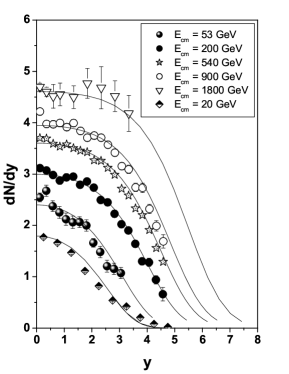
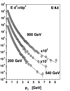
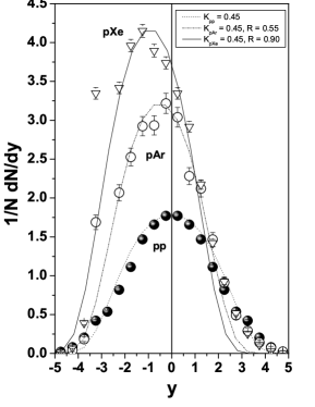
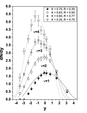
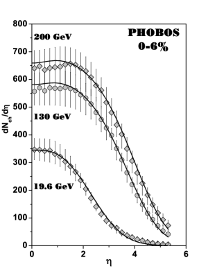
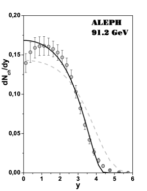
Figure 1: Examples of application of IT approach to different kind of data. Top-left: $dN/dy$ for $pp$ and $\bar{p}p$ collisions at different energies, fitted parameters are inelasticity and $q=q_{L}$, cf., [6] for details. Top-middle: $p_{T}$ distributions at different energies [7] (fitted parameter is $q=q_{T}$ which remains much smaller than $q_{L}$. Top-right: $dN/dy$ in the so called ”tube model” of $pA$ collisions, here $K$ and $R$ are fraction of energies of, respectively, incoming nucleon and ”tube” used in hadronization process, cf., [8] for details. Bottom-left: $p-(\nu)$nucleonic rapidity distributions for different values of hit nucleons in the tube model [8]. Notice that data on collisions of incoming proton with nuclear nucleon ( $\nu=1$) disagree with data for $pp$ collision at the same energy (lowest curve at upper-left panel) and cannot be therefore fitted - the probably reason is that ”nucler nucleon” is a mixture of $p$ and $n$. Bottom-middle: $dN/d\eta$ distributions in $AA$ collisions [9]. Bottom-right: attempt to fit $e^{+}e^{-}$ data - as one can see they cannot be fitted properly by IT the method, cf. [9]. Here the best fit is for $q<1$ which therefore limits available phase space.

4 Summary

The question arises: what is the advantage of the IT method? To answer it let us first notice that in examples presented in Fig. 1 IT was represented by most probable and least biased distribution (6) describing allocation of given (known) number of secondaries in a (longitudinal) phase space defined by a given (or assumed, by using parameter of inelasticity $K$) available energy. It means then that [2, 6] in (6) one has only one term, $k=1$, with $F_{1}$ being energy of secondary under consideration and the lagrange multiplier $\lambda_{1}=\beta$, being the inverse of ”temperature” (understood in the sense mentioned before). This formula is apparently identical with formula used by statistical models of hadronization, however, here both $\beta$ and $Z$ are not free parameters (see [6] for discussion and references) but are obtained from the constraint equations (here energy conservation and normalization). The parameters fitted is the energy available for hadronization (i.e., inelasticity parameter $K$, cf., [2, 6], in some cases like $e^{+}e^{-}$ collisions and some $AA$ collisions they are fixed by the requirement of experiment) and parameter $q$, which as we argue, defines the amount of dynamical, intrinsic fluctuations present in the hadronizing system. In case that data cannot be fitted by this method we should add some other constraints (as in $pA$ case [8]), or turn to the true dynamical description (as is probably the case with $e^{+}e^{-}$ collisions).

Let us end with remark that IT does not solve our dynamical problems. On the other hand it is the only approach which allows us to select a minimal number of indispensable hypothesis (assumptions) needed to reproduce experimental data under consideration. In this approach any new hypothesis are allowed only when discrepancy with some new (or additional) experimental results occur. The choice of the form of information entropy (here represented by parameter $q$) offers additional flexibility because, as was stressed here, $q$ summarizes many possible dynamical effects (out of which we have stressed here fluctuations). Therefore assumptions tested by using methods of IT can serve as ideal starting point to build any dynamical model of hadronization process.

Two of us (OU and GW) would like to acknowledge support obtained from the Bogolyubov-Infeld program in JINR. Partial support of the Polish State Committee for Scientific Research (KBN) (grant 621/E-78/SPUB/CERN/P-03/DZ4/99 (GW)) is also acknowledged.

References

- [1] Y.-A.Chao, Nucl. Phys. B40 (1972) 475.
- [2] G.Wilk and Z.Włodarczyk, Phys. Rev. D43 (1991) 794.
- [3] F. Topsœ, Physica A340 (2004) 11.
- [4] C. Tsallis, in Nonextensive Statistical Mechanics and its Applications, S.Abe and Y.Okamoto (Eds.), Lecture Notes in Physics LPN560, Springer (2000), in Physica A340 (2004) 1 and Physica A344 (2004) 718, and references therein.
- [5] A.M. Teweldeberhan, H.G. Miller and R. Tegen, Int. J. Mod. Phys. E12 (2003) 395.
- [6] F.S. Navarra, O.V. Utyuzh, G. Wilk and Z. Włodarczyk, Phys. Rev. D67 (2003) 114002.
- [7] F.S. Navarra, O.V. Utyuzh, G. Wilk and Z. Włodarczyk, Physica A340 (2004) 467.
- [8] O.V.Utyuzh, G.Wilk and Z.Włodarczyk, Multiparticle production processes from the Information Theory point of view, hep-ph/0503048, to be published in Acta Phys. Hung. A (HIP) (2005).
- [9] F.S. Navarra, O.V. Utyuzh, G. Wilk and Z. Włodarczyk, Physica A344 (2004) 568.
- [10] G.Wilk and Z.Włodarczyk, Phys. Rev. Lett. 84 (2000) 2770; Chaos, Solitons and Fractals 13 (2002) 581 and Physica A305 (2002) 227.
- [11] C. Beck and E.G.D. Cohen, Physica A322 (2003) 267.
- [12] M. Biyajima, M. Kaneyama, T. Mizoguchi and G. Wilk, Eur. Phys. J. C40 (2005) 243.
- [13] P. Carruthers and C.C. Shih, Int. J. Mod. Phys. A4 (1989) 5587.
- [14] O.V. Utyuzh, G. Wilk and Z. Włodarczyk, J. Phys. G26 (2000) L39.
- [15] C.Tsallis, M. Gell-Mann and Y.Sato, Asymptotically scale-invariant occupancy of phase space makes the entropy Sq extensive, cond-mat/0502274; T.S.Biró, G.Purcsel, G.Györgyi, A.Jakovác and Z.Schramd, Power-law tailed spectra from equilibrium; nucl-th/0510008, talk given at QM2005, Budapest (and references therein).