This talk consists of two parts. In the first, the present experimental bounds on the anomalous couplings of the gauge bosons, based mainly on the LEP and Tevatron experiments, are reviewed. In the second part, the theorem of helicity conservation (HC) is presented, which should be valid in either the Standard Model (SM) or MSSM, for any two-body process at high energies and fixed angles. The energy-range for the HC validity is discussed and, under certain conditions, it should well be within the LHC or ILC range. Since all known anomalous couplings violate HC, its testing may provide a way for generically identifying the possible presence of anomalous (non-renormalizable) contributions.

1 Introduction

The description of particle physics through renormalizable $SU(3)\times SU(2)\times U(1)$ gauge invariant interactions, has been impressively successful, up to now.

The keyword here is renormalizable, which imposes that only operators of dimensions less than or equal to four, can appear in the Lagrangian. This property, together with the group structure, determine the gauge and matter interactions, leading e.g. to the most striking phenomenon of asymptotic freedom which permeates contemporary particle and cosmology physics [1].

In order to thoroughly test experimentally these interactions, alternative models are envisaged, which may be used as parameterizations of any possible violation of their validity. As such, in the present context we consider anomalous gauge couplings [2, 3, 4]. These anomalous couplings can always be assumed to obey $SU(3)\times SU(2)\times U(1)$ symmetry [5]; but, due to their higher dimensionality, they violate renormalizability.

Extensive phenomenological studies have already been made in various specific processes, comparing the signatures of such couplings, to those of e.g. the Standard Model (SM). On the basis of these, experimental searches have been performed at LEP, the Tevatron and elsewhere; which invariably impose ever growing constraints on the magnitude of any conceivable anomalous coupling. Thus, at present at least, SM (as well as its renormalizable SUSY extensions), are fully consistent with Nature.

The strength of these constraints will most probably further increase when LHC or ILC start operating, basically because the non-renormalizable nature of the anomalous couplings bounds their effects to increase strongly with energy. Such a strong increase is in fact a common feature of all effectively non-renormalizable ways of going beyond SM or its SUSY analogs. In turn, this facilitates their exclusion, provided of course we adhere to the usual practice of considering e.g. only a few anomalous couplings at a time.

As the energy increases reaching the LHC range though, it becomes increasingly difficult to motivate the idea that the anomalous couplings may be parameterized by a few dimension=6 operators only. Instead, higher dimensional operators (as well as previously ignored dim=6 ones) should be considered together; particularly if the scale of new physics is reached there, thereby seriously reducing the ability to constrain the anomalous couplings.

A partial solution to this difficulty is offered by the property called helicity conservation (HC), which in SM and its renormalizable SUSY extensions, greatly reduces the number of non-vanishing amplitudes at very high energies and fixed angles [6]. Combining this with the observation that all known anomalous couplings violate HC, we obtain a generic test for all of them.

The importance of HC as a property of SM and MSSM, and in fact of any renormalizable gauge theory, can hardly be overemphasized. Its validity, particularly for gauge amplitudes in SM, is only established after large cancellation from different diagrams, which are only realized for renormalizable couplings [6]. Because of this, HC is not directly obvious from the SM Lagrangian, and it must somehow be related to the twistor structure in QCD [7]. The possible appearance of HC violation indicates the presence of some non-renormalizable contributions, an example of which is of course the anomalous couplings [6].

In the first part of this talk I review the present constraints on the anomalous gauge couplings; while in the second part, HC is described.

2 Anomalous electroweak couplings

As is well known, anomalous electroweak couplings may be introduced in SM or MSSM by including operators of higher than four dimension, which preserve the $SU(3)\times SU(2)\times U(1)$ gauge symmetry. These operators induce anomalous couplings not only to the gauge bosons, but also to the Higgs particles [8], and the quarks and leptons, particularly of the third family [9]. Since no Higgs particle has yet been discovered, and the top anomalies are covered by J. Wudka [10], we will concentrate here on the purely gauge anomalous couplings.

2.1 $W^{\pm}$ anomalous Couplings

The most general set of the anomalous triple gauge couplings (TGC) describing all possible $(W^{+}W^{-}Z)$ and $(W^{+}W^{-}\gamma)$ vertices, is traditionally parameterized as [2, 3, 4]

$${\cal L}^{\rm TGC}_{NP} = -ieg_{VWW}\Big{\{}(1+\delta g_{1}^{V})V^{\mu}(W^{-}_{\mu\nu}W^{+\nu}-W^{+}_{\mu\nu}W^{-\nu})+(1+\delta\kappa_{V})V^{\mu\nu}W^{+}_{\mu}W^{-}_{\nu}$$ (1)

$$+ \frac{\lambda_{V}}{m_{W}^{2}}V^{\mu\nu}W^{+\rho}_{\nu}W^{-}_{\rho\mu}+ig_{5}^{V}\epsilon_{\mu\nu\rho\sigma}[(\partial^{\rho}W^{-\mu})W^{+\nu}-W^{-\mu}(\partial^{\rho}W^{+\nu})]V^{\sigma}$$

$$+ ig_{4}^{V}W^{-}_{\mu}W^{+}_{\nu}(\partial^{\mu}V^{\nu}+\partial^{\nu}V^{\mu})-\tilde{\kappa}_{V}W^{-}_{\mu}W^{+}_{\nu}\tilde{V}_{\mu\nu}-\frac{\tilde{\lambda}_{V}}{m_{W}^{2}}W^{-}_{\rho\mu}W^{+\mu}\tilde{V}^{\nu\rho}\Big{\}}~{},$$

where

$$\tilde{V}_{\mu\nu}=\frac{1}{2}\epsilon_{\mu\nu\rho\sigma}V^{\rho\sigma}~{}~{},~{}~{}$$

$$V=\gamma~{},~{}Z~{}~{}~{}~{}\leftrightarrow~{}~{}~{}~{}g_{\gamma WW}=1~{},~{}g_{ZWW}=\frac{c_{W}}{s_{W}}~{}~{}.$$ (2)

The anomalous couplings $(\delta g_{1}^{V}~{},~{}\delta\kappa_{V}~{},~{}\lambda_{V}~{},~{}g_{5}^{V})$ respect CP, while $(g_{4}^{V}~{},~{}\tilde{\kappa}_{V}~{},~{}\tilde{\lambda}_{V})$ violate it. For the photon couplings in particular, $U_{\rm em}(1)$ gauge invariance implies that

$$\delta g_{1}^{\gamma}\sim\frac{q^{2}}{\Lambda^{2}}~{}~{},~{}~{}g_{5}^{\gamma}\sim\frac{q^{2}}{\Lambda^{2}}~{}~{},~{}~{}g_{4}^{\gamma}\sim\frac{q^{2}}{\Lambda^{2}}~{}~{},$$

as the off-shell photon approaches its mass shell value $q^{2}=0$.

The phases in the effective lagrangian (1) have been chosen so that all couplings are real, in case the scale of the new physics (NP) inducing them is very high. If the NP scale is low though, pole and branch-point singularities develop.

All anomalous TGC are consistent with $SU(3)\times SU(2)\times U(1)$ gauge invariance, provided they are combined with appropriate interactions involving more gauge and/or physical Higgs particles. To achieve this for the actual couplings in (1) though, operators of dimension up to 12 need be considered [5].

Of course, if the NP scale is not very high, like e.g. in a SUSY case with the new particles at the LHC range, operators of any dimension would be allowed, seriously weakening our ability to constrain them.

If, on the contrary, the NP scale is high though, and the physical Higgs particles are within the electroweak range, then the natural couplings of the induced operators should be $g_{0}\sim 1/\Lambda^{{\rm dim}-4}$, allowing the contemplation that dimension=6 operators could be sufficient in describing NP.

Disregarding all such operators which are strongly excluded due to their tree-level contributions to physical observables, and assuming also that only one SM-like light Higgs particle exists, we parameterize the anomalous contribution to the effective lagrangian describing the $W^{\pm}$ TGC as [12]

$${\cal L}^{\rm TGC}_{NP}({\rm dim}=6) = \frac{e}{c_{W}m_{W}^{2}}\alpha_{B\phi}{\cal O}_{B\phi}+\frac{e}{s_{W}m_{W}^{2}}\alpha_{W\phi}{\cal O}_{W\phi}+\frac{e}{s_{W}m_{W}^{2}}\alpha_{W}{\cal O}_{W}$$ (3)

$$+ \frac{e^{2}}{2s_{W}c_{W}m_{W}^{2}}\tilde{\alpha}_{BW}\tilde{\cal O}_{BW}+\frac{e}{s_{W}m_{W}^{2}}\tilde{\alpha}_{W}\tilde{\cal O}_{W}~{}~{},$$

with

$${\cal O}_{W}=\frac{1}{3!}(\vec{W}_{\mu\nu}\times\vec{W}^{\nu\lambda})\cdot\vec{W}_{\lambda}^{~{}\mu}~{}~{}, {\cal O}_{W\phi}=iD_{\mu}\phi^{\dagger}\vec{\tau}\vec{W}^{\mu\nu}D_{\nu}\phi ~{},~{}~{}{\cal O}_{B\phi}=iD_{\mu}\phi^{\dagger}B^{\mu\nu}D_{\nu}\phi~{}~{},$$

$$\tilde{\cal O}_{W}=\frac{1}{3!}(\vec{W}_{\mu\nu}\times\vec{W}^{\nu\lambda})\cdot\tilde{\vec{W}}_{\lambda}^{~{}\mu}~{}~{}, \tilde{\cal O}_{W\phi}=\frac{i}{2}\phi^{\dagger}\vec{\tau}\tilde{\vec{W}}^{\mu\nu}\phi B_{\mu\nu} ~{},$$ (4)

where the first three operators conserve CP, while the rest two violate it. The anomalous couplings defined in (1), are related to those in (3), by

$$\delta g_{1}^{Z}=\frac{\alpha_{W\phi}}{c^{2}_{W}}~{}~{},~{}~{}\lambda_{\gamma}=\lambda_{Z}=\alpha_{W}~{}~{},~{}~{}\delta\kappa_{\gamma}=-\frac{c^{2}_{W}}{s^{2}_{W}}(\delta\kappa_{Z}-\delta g_{1}^{Z})=\alpha_{W\phi}+\alpha_{B\phi}~{}~{},$$

$$\tilde{\kappa}_{\gamma}=-\frac{c^{2}_{W}}{s^{2}_{W}}\tilde{\kappa}_{Z}=\tilde{\alpha}_{BW}~{}~{},~{}~{}\tilde{\lambda}_{\gamma}=\tilde{\lambda}_{Z}=\tilde{\alpha}_{W}~{}~{}.$$ (5)

Restricting to CP conserving couplings only, and using the definitions

$$\kappa_{\gamma}\equiv 1+\delta\kappa_{\gamma}~{}~{},~{}~{}\kappa_{Z}\equiv 1+\delta\kappa_{Z}~{}~{},~{}~{}g_{1}^{V}\equiv 1+\delta g_{1}^{V}~{}~{},~{}~{}$$

we end up in a situation where only the three independent couplings

$$~{}~{}g_{1}^{Z}~{}~{},~{}~{}\kappa_{\gamma}~{}~{},~{}~{}\lambda_{\gamma}$$ (6)

participate, whose standard values are (1,1,0) respectively. The fitted LEP ranges for these parameters from [13] are indicated in Fig.1 and Table 1, obtained respectively by varying two or one parameter at a time.

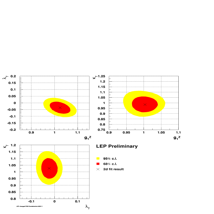
Figure 1: The combined LEP2 results from [13]. In each case two of the parameters in (6) are varied, while the third is fixed at its standard value.

Parameter	68% C.L.	95% C.L.
$g_{1}^{Z}$	$0.991^{0.022}_{0.021}$	[$0.949,~{}~{}1.034$]
$\kappa_{\gamma}$	$0.984^{0.042}_{0.047}$	[$0.895,~{}~{}1.069$]
$\lambda_{\gamma}$	$-0.016^{0.021}_{0.023}$	[$-0.059,~{}~{}0.026$]

Table 1: The combined LEP2 results from [13]. In each case the listed parameter is varied while the other two of (6) are fixed to their standard values.

The corresponding one-parameter Tevatron D0 fits from [14], are given in Table 2. Due to the large energy scale there, the anomalous couplings are replaced by form factors as e.g. $\lambda_{Z}\to\lambda_{Z}/(1+\hat{s}/\Lambda^{2})$, and the presented fits correspond to $\Lambda=1$ and 1.5 TeV.

Condition	$\Lambda$ = 1 TeV	$\Lambda$ = 1.5 TeV
$\Delta g^{Z}_{1}=\Delta\kappa_{Z}=0$	$-0.53<\lambda_{Z}<0.56$	$-0.48<\lambda_{Z}<0.48$
$\lambda_{Z}=\Delta\kappa_{Z}=0$	$-0.57<\Delta g^{Z}_{1}<0.76$	$-0.49<\Delta g^{Z}_{1}<0.66$
$\lambda_{Z}=0$	$-0.49<\Delta g_{1}^{Z}=\Delta\kappa_{Z}<0.66$	$-0.43<\Delta g_{1}^{Z}=\Delta\kappa_{Z}<0.57$
$\lambda_{Z}=\Delta g^{Z}_{1}=0$	$-2.0<\Delta\kappa_{Z}<2.4$	$-$

Table 2: One-parameter 95% C.L. fits from D0 [14].

As usual, the $W^{\pm}$ TGC constraints become stronger with energy. Thus, even stronger constrains are expected at LHC and ILC. One additional reason for this, applying to the specific operators ${\cal O}_{W},{\cal O}_{W\phi},\tilde{\cal O}_{W}$ in (4), is that they also produce quartic couplings of the form $WW\gamma\gamma$, $WWZ\gamma$, $WWZZ$, which may also be measured [15].

Eventually, these constraints will become so strong, particularly for ILC, that 1-loop or higher SM results will be needed for correctly taking into account the ”SM-background”.

2.2 The on-shell anomalous triple neutral gauge couplings

Using Fig.2 and [3, 16], the general triple neutral gauge vertex is written as

Figure 2: The definition of the general triple neutral gauge boson vertex, with $V_{1},V_{2}$ taken on-shell, while $V_{3}$ is generally off shell.

$$\Gamma^{\alpha\beta\mu}_{ZZV}(q_{1},q_{2},P) = \frac{i(s-m_{V}^{2})}{m_{Z}^{2}}\left[f_{4}^{V}(P^{\alpha}g^{\mu\beta}+P^{\beta}g^{\mu\alpha})-f_{5}^{V}\epsilon^{\mu\alpha\beta\rho}(q_{1}-q_{2})_{\rho}\right]~{},$$ (7)

$$\Gamma^{\alpha\beta\mu}_{Z\gamma V}(q_{1},q_{2},P) = \frac{i(s-m_{V}^{2})}{m_{Z}^{2}}\Bigg{\{}h_{1}^{V}(q_{2}^{\mu}g^{\alpha\beta}-q_{2}^{\alpha}g^{\mu\beta})+\frac{h_{2}^{V}}{m_{Z}^{2}}P^{\alpha}[(Pq_{2})g^{\mu\beta}-q_{2}^{\mu}P^{\beta}]$$ (8)

$$- h_{3}^{V}\epsilon^{\mu\alpha\beta\rho}q_{2\rho}~{}-~{}\frac{h_{4}^{V}}{m_{Z}^{2}}P^{\alpha}\epsilon^{\mu\beta\rho\sigma}P_{\rho}q_{2\sigma}\Bigg{\}}~{},$$

where $(V_{3}=Z,\gamma)$ is generally off-shell, while the other two neutral gauge bosons are always on-shell. If the NP scale is very high, all couplings in (7,8) are real. Singularities develop only if the NP scale is nearby. The couplings $(f_{5}^{V},h_{3}^{V},h_{4}^{V})$ respect CP, while $(f_{4}^{V},h_{1}^{V},h_{2}^{V})$ violate it. Finally, the $(h_{2}^{V},h_{4}^{V})$-interactions may be relatively suppressed, since they are of higher dimension.

Based on [13], the fitted LEP ranges for the $ZZ$-production couplings are indicated in Table 3, for the cases that only one or only two anomalous couplings are possibly non-vanishing. The corresponding results for $Z\gamma$ production at LEP are given in Table 4 [13]; while the D0 results appear in Table 5.

Parameter	95% C.L.
$f_{4}^{\gamma}$	[$-0.17,~{}~{}+0.19$]
$f_{4}^{Z}$	[$-0.30,~{}~{}+0.30$]
$f_{5}^{\gamma}$	[$-0.32,~{}~{}+0.36$]
$f_{5}^{Z}$	[$-0.34,~{}~{}+0.38$]

Parameter	95% C.L.	Correlations
$f_{4}^{\gamma}$	[$-0.17,~{}~{}+0.19$]	$1.00$	$0.07$
$f_{4}^{Z}$	[$-0.30,~{}~{}+0.29$]	$0.07$	$1.00$
$f_{5}^{\gamma}$	[$-0.34,~{}~{}+0.38$]	$1.00$	$-0.17$
$f_{5}^{Z}$	[$-0.38,~{}~{}+0.36$]	$-0.17$	$1.00$

Table 3: The fitted parameters for the anomalous neutral TGC from the LEP $ZZ$ production [13]. Only the listed parameters are varied in each case; one in the left panel and two in the right one. In each case, the non-listed parameters are vanishing.

Parameter	95% C.L.
$h_{1}^{\gamma}$	[$-0.056,~{}~{}+0.055$]
$h_{2}^{\gamma}$	[$-0.045,~{}~{}+0.025$]
$h_{3}^{\gamma}$	[$-0.049,~{}~{}-0.008$]
$h_{4}^{\gamma}$	[$-0.002,~{}~{}+0.034$]
$h_{1}^{Z}$	[$-0.13,~{}~{}+0.13$]
$h_{2}^{Z}$	[$-0.078,~{}~{}+0.071$]
$h_{3}^{Z}$	[$-0.20,~{}~{}+0.07$]
$h_{4}^{Z}$	[$-0.05,~{}~{}+0.12$]

Parameter	95% C.L.	Correlations
$h_{1}^{\gamma}$	[$-0.16,~{}~{}+0.05$]	$1.00$	$+0.79$
$h_{2}^{\gamma}$	[$-0.11,~{}~{}+0.02$]	$+0.79$	$1.00$
$h_{3}^{\gamma}$	[$-0.08,~{}~{}+0.14$]	$1.00$	$+0.97$
$h_{4}^{\gamma}$	[$-0.04,~{}~{}+0.11$]	$+0.97$	$1.00$
$h_{1}^{Z}$	[$-0.35,~{}~{}+0.28$]	$1.00$	$+0.77$
$h_{2}^{Z}$	[$-0.21,~{}~{}+0.17$]	$+0.77$	$1.00$
$h_{3}^{Z}$	[$-0.37,~{}~{}+0.29$]	$1.00$	$+0.76$
$h_{4}^{Z}$	[$-0.19,~{}~{}+0.21$]	$+0.76$	$1.00$

Table 4: The fitted parameters for the anomalous neutral TGC from the LEP $Z\gamma$ production [13]. Only the listed parameters are varied in each case; one in the left panel and two in the right one. In each case, the non-listed parameters are vanishing.

Coupling	$\Lambda=$ 750 GeV	$\Lambda=$ 1 TeV
$|\Re{\it e}(h_{10,30}^{Z})|$, $|\Im{\it m}(h_{10,30}^{Z})|$	0.24	0.23
$|\Re{\it e}(h_{20,40}^{Z})|$, $|\Im{\it m}(h_{20,40}^{Z})|$	0.027	0.020
$|\Re{\it e}(h_{10,30}^{\gamma})|$, $|\Im{\it m}(h_{10,30}^{\gamma})|$	0.29	0.23
$|\Re{\it e}(h_{20,40}^{\gamma})|$, $|\Im{\it m}(h_{20,40}^{\gamma})|$	0.030	0.019

Table 5: The fitted parameters for the anomalous neutral TGC from the D0 $Z\gamma$ production [17]. Only the listed parameters are varied in each case, which are taken to be either purely real or purely imaginary. In each case, the non-listed parameters are vanishing.

The overall conclusion on the basis of Fig.1 and Tables 1-5, is that no indication for any anomalous TGC exists at present.

3 Helicity Conservation and its possible violation.

We next turn to the Helicity Conservation (HC) property, restricting to processes of even order in the Yukawa couplings [6]. Simple rules are then obtained, that generically test the presence of anomalous couplings for any two-body process at high energies and fixed angles [6]. Thus, denoting its helicity amplitudes by $F(a_{\lambda_{1}}b_{\lambda_{2}}\to c_{\lambda_{3}}d_{\lambda_{4}})$, the allowed helicities at asymptotic $(s,|t|,|u|)$-values are constrained as

$$\lambda_{1}+\lambda_{2}=\lambda_{3}+\lambda_{4}~{}~{},$$ (9)

unless the two initial (or final) particles are fermions and the other two bosons, where the stronger relation

$$\lambda_{1}+\lambda_{2}=\lambda_{3}+\lambda_{4}=0~{}~{}$$ (10)

is imposed.

Particularly for transverse gauge bosons, the structure for the asymptotically non-vanishing two-body helicity amplitudes implied by HC is

$$F(f_{\lambda_{f}}f^{\prime}_{\lambda_{-f}}\to V_{\lambda_{V}}V^{\prime}_{\lambda_{-V}})~{}~{},~{}~{}F(V_{\lambda_{V}}V^{\prime}_{\lambda_{-V}}\to f_{\lambda_{f}}f^{\prime}_{\lambda_{-f}})~{}~{},$$ (11)

$$F(V_{\lambda_{V}}V^{\prime}_{\lambda_{-V}}\to\phi\phi^{\prime})~{}~{},~{}~{}F(\phi\phi^{\prime}\to V_{\lambda_{V}}V^{\prime}_{\lambda_{-V}})~{}~{},$$ (12)

$$F(V_{\lambda_{V}}f_{\lambda_{f}}\to V^{\prime}_{\lambda_{V}}f^{\prime}_{\lambda_{f}})~{}~{},~{}~{}F(V_{\lambda_{V}}\phi\to V^{\prime}_{\lambda_{V}}\phi^{\prime})~{}~{},~{}~{}$$ (13)

where by $f,\phi,V$ we denote fermion, scalar or vector particles respectively.

Equations (9, 10) remain of course true even in the presence of longitudinal vector bosons. For the vector boson amplitudes denoted as $F(V^{1}_{\lambda_{1}}V^{2}_{\lambda_{2}}\to V^{3}_{\lambda_{3}}V^{4}_{\lambda_{4}})\equiv F_{\lambda_{1}\lambda_{2}\lambda_{3}\lambda_{4}}$, they also imply relations like

$$F_{+++-}=F_{++-+}=F_{+-++}=F_{-+++}=F_{---+}$$

$$=F_{++LL}=F_{-+-L}=F_{+--L}=F_{++L-}\simeq 0~{}~{},$$ (14)

since all HC-violating amplitudes should necessarily vanish at high $(s,|t|,|u|)$.

The most important ingredient for the validity of HC in either SM or MSSM, is renormalizability [6].

For processes involving fermions or scalars only, HC holds at a diagram-by-diagram basis. For gauge involving amplitudes though, the situation is more subtle. Large cancellations among the various diagrams are needed in order to achieve HC. This way, HC is established at the Born level in both SM and MSSM. When going beyond this though, intriguing differences between SM and MSSM appear, which we summarize below.

In SM, HC is only valid up to the $\ln^{2}$ and $\ln$ terms of the 1-loop corrections, provided $(s,|t|,|u|)\gg(m_{W}^{2},m^{2}_{H})$. The theorem is easier to be established for processes driven by a non-vanishing Born contribution. In any case, it has been checked explicitly to the leading log accuracy, for $(e^{-}e^{+}\to\gamma\gamma,~{}ZZ,~{}\gamma Z,~{}W^{-}W^{+})$ using [18], and $(\gamma\gamma\to ZZ,~{}\gamma Z,~{}ZZ)$ using [19, 20, 21]. Constant high energy contributions in SM though, usually violate HC.

In MSSM, HC is valid to all orders in the gauge and Yukawa couplings, for any two-body process, at $(s,|t|,|u|)\gg M_{\rm SUSY}^{2}$ [6]. Constant contributions respect it also!

SUSY somehow knows of the cancellations among the various diagrams describing the gauge boson involving processes. The reason for this is that, at high energies SUSY associates each gauge boson of a definite helicity, to a corresponding gaugino carrying a helicity of the same sign. Since, HC is valid for fermions at a diagram-by-diagram basis; it should be valid for gauge bosons also. In the general proof, masses have been neglected [6].

The validity of HC, even for the constant asymptotic contributions in MSSM, has also been observed in $\gamma\gamma\to ZZ,~{}\gamma Z,~{}ZZ$, for which the exact 1-loop results are known [6, 20, 21].

	$\tau=\tau^{\prime}=\pm 1$	$\tau=-\tau^{\prime}=\pm 1$	$\tau=\tau^{\prime}=0$	$\tau=0,\tau^{\prime}=\pm 1,\epsilon=1$
	$-\frac{e^{2}}{2}\lambda\sin\theta$	$-\frac{e^{2}}{2}\lambda\sin\theta$	$-\frac{e^{2}}{2}\lambda\sin\theta$	$-e^{2}\lambda\frac{(\tau^{\prime}\cos\theta-2\lambda)}{2\sqrt{2}}$
$\delta_{Z}$	$-2\delta_{Z}(a-2b\lambda)$	0	$-\frac{s}{m_{W}^{2}}\delta_{Z}(a-2b\lambda)$	$-\frac{\sqrt{s}}{m_{W}}2\delta_{Z}(a-2b\lambda)$
$x_{\gamma}~{},x_{Z}$	0	0	$\frac{s}{m_{W}^{2}}[x_{\gamma}-x_{Z}(a-2b\lambda)]$	$\frac{\sqrt{s}}{m_{W}}[x_{\gamma}-x_{Z}(a-2b\lambda)]$
$y_{\gamma}~{},y_{Z}$	$\frac{s}{m_{W}^{2}}[y_{\gamma}-y_{Z}(a-2b\lambda)]$	0	0	$\frac{\sqrt{s}}{m_{W}}[y_{\gamma}-y_{Z}(a-2b\lambda)]$
$z_{Z}$	0	0	0	$-\Big{(}\frac{\sqrt{s}}{m_{W}}\Big{)}^{3}z_{Z}(a-2b\lambda)\tau^{\prime}$
$z^{\prime}_{1}$	0	0	0	$-i\frac{\sqrt{s}}{m_{W}}z^{\prime}_{1}(a-2b\lambda)\epsilon$
$z^{\prime}_{2}$	$iz^{\prime}_{2}2\tau(a-2b\lambda)$	0	0	$i\frac{\sqrt{s}}{m_{W}}z^{\prime}_{2}\tau^{\prime}(a-2b\lambda)\epsilon$
$z^{\prime}_{3}$	$-iz^{\prime}_{3}2\tau(a-2b\lambda)\frac{s}{m_{W}^{2}}$	0	0	0

Table 6: The leading large-s anomalous contribution to $F(e^{-}_{\lambda}e^{+}_{-\lambda}\to W^{-}_{\tau}W^{+}_{\tau^{\prime}})$ [22]. The helicity amplitudes are obtained from each column by multiplying the factor on top, with the sum of all its elements. The first column indicates the anomalous couplings contributing. The amplitudes for $\tau=\pm 1,\tau^{\prime}=0$ are obtained from the last column by substituting there $\tau^{\prime}\to-\tau$ and $\epsilon=-1$.

We next turn to the anomalous contributions to the asymptotic two-body amplitudes. Since the most we can expect about such couplings is that they are very small, we always calculated their contribution at the Born level. For $F(e^{-}_{\lambda}e^{+}_{-\lambda}\to W^{-}_{\tau}W^{+}_{\tau^{\prime}})$, the complete asymptotic anomalous contributions to the helicity amplitudes are given in Table 6 [22], where (1) and the definitions

$$a=\frac{-1+4s^{2}_{W}}{4s_{W}c_{W}}~{}~{},~{}~{}b=\frac{-1}{4s_{W}c_{W}}~{}~{},~{}~{}\delta_{Z}=\frac{c_{W}}{s_{W}}\delta g_{1}^{Z}~{}~{},$$

$$x_{\gamma}=\delta\kappa_{\gamma}~{}~{},~{}~{}x_{Z}=(\delta\kappa_{Z}-\delta g_{1}^{Z})\frac{c_{W}}{s_{W}}~{}~{},~{}~{}y_{\gamma}=\lambda_{\gamma}~{}~{},~{}~{}y_{Z}=\lambda_{Z}\frac{c_{W}}{s_{W}}~{}~{}$$ (15)

are used. The CP violating couplings $(z^{\prime}_{1},z^{\prime}_{2},z^{\prime}_{3})$ in the last three rows of Table 6, are linear combinations of the couplings $(g_{4}^{Z},\tilde{\kappa}_{Z},\tilde{\lambda}_{Z})$ defined in (1) [22].

As seen from Table 6, none of the TGC in (1), respects HC. Thus, bounds on the ratios

$$\frac{|F(e^{-}_{\lambda}e^{+}_{-\lambda}\to W^{-}_{0}W^{+}_{\pm 1})|}{|F(e^{-}_{\lambda}e^{+}_{-\lambda}\to W^{-}_{\pm 1}W^{+}_{\mp 1})|} \frac{|F(e^{-}_{\lambda}e^{+}_{-\lambda}\to W^{-}_{\pm 1}W^{+}_{0})|}{|F(e^{-}_{\lambda}e^{+}_{-\lambda}\to W^{-}_{\pm 1}W^{+}_{\mp 1})|}~{}~{},$$ ,

$$\frac{|F(e^{-}_{\lambda}e^{+}_{-\lambda}\to W^{-}_{\pm 1}W^{+}_{\pm 1})|}{|F(e^{-}_{\lambda}e^{+}_{-\lambda}\to W^{-}_{\pm 1}W^{+}_{\mp 1})|} \frac{|F(e^{-}_{\lambda}e^{+}_{-\lambda}\to W^{-}_{0}W^{+}_{0})|}{|F(e^{-}_{\lambda}e^{+}_{-\lambda}\to W^{-}_{\pm 1}W^{+}_{\mp 1})|}~{}~{},$$ ,

measured at the high energy part of Linear Collider (ILC), could constrain all anomalous couplings.

As further examples of anomalous HC violations in other 2-body processes, we give in (16-21), the SM and ${\cal O}_{W}$ contributions to the high energy helicity amplitudes [23]; compare (3, 4). In all cases, the HC violating amplitudes, indicated through a double arrow in the left hand sides of (16-21), are determined by the anomalous interactions. These are

$d\bar{d},\ u\bar{u}\to W^{-}W^{+}$

$$\Rightarrow~{}~{}F^{L}_{++}=F^{L}_{--}=\>\tau_{3}\>{e^{2}\over 4s^{2}_{W}}\biggm{(}{\alpha_{W}s\over m_{W}}\biggm{)}\sin\theta$$

$$F^{L}_{+-}=-{e^{2}\over 2s^{2}_{W}}\sin\theta\>{(1-\tau_{3}\cos\theta)\over 1+\cos\theta}\ \ \ ;\ \ F^{L}_{-+}={e^{2}\over 2s^{2}_{W}}\sin\theta\>{(1-\tau_{3}\cos\theta)\over 1-\cos\theta}$$

$$F^{L}_{LL}=\tau_{3}{e^{2}\over 2c^{2}_{W}}\sin\theta\>(|Q|-1+{1\over 2s^{2}_{W}})$$

$$F^{R}_{LL}=Q{e^{2}\over 2c^{2}_{W}}\sin\theta~{}~{},$$ (16)

where $Q$ is the quark charge,

$d\bar{u}\to W^{-}Z$

$$\Rightarrow~{}~{}F^{L}_{++}=F^{L}_{--}=-\>{e^{2}\over 2\sqrt{2}}\>{c_{W}\over s^{2}_{W}}\>\biggm{(}{\alpha_{W}s\over m_{W}}\biggm{)}\sin\theta$$

$$F^{L}_{+-}=-\>{e^{2}\over\sqrt{2}c_{W}s^{2}_{W}}\>\>{\sin\theta\over 1+\cos\theta}\ \bigm{(}c^{2}_{W}\cos\theta-{s^{2}_{W}\over 3}\bigm{)}$$

$$F^{L}_{-+}={e^{2}\over\sqrt{2}c_{W}s^{2}_{W}}\>\>{\sin\theta\over 1-\cos\theta}\ \bigm{(}c^{2}_{W}\cos\theta-{s^{2}_{W}\over 3}\bigm{)}$$

$$F^{L}_{LL}=-\>{e^{2}\over 2\sqrt{2}\,s^{2}_{W}}\>\sin\theta~{}~{},$$ (17)

$d\bar{u}\to W^{-}\gamma$

$$\Rightarrow~{}~{}F^{L}_{++}=F^{L}_{--}=\>-\>{e^{2}\over 2\sqrt{2}\,s_{W}}\>\sin\theta\biggm{(}{\alpha_{W}s\over m_{W}}\biggm{)}$$

$$F^{L}_{+-}=-\>{e^{2}\over\sqrt{2}\,s_{W}}\ \ {\sin\theta\over 1+\cos\theta}\ \bigm{(}\cos\theta+{1\over 3}\bigm{)}$$

$$F^{L}_{-+}={e^{2}\over\sqrt{2}\,s_{W}}\ \ {\sin\theta\over 1-\cos\theta}\ \bigm{(}\cos\theta+{1\over 3}\bigm{)}~{}~{},$$ (18)

$\gamma\gamma\to WW$

$$F_{++++}=F_{----}=\ {8e^{2}\over\sin^{2}\theta}$$

$$\Rightarrow~{}~{}F_{+++-}=F_{++-+}=\ F_{+-++}=\ F_{-+++}=$$

$$\Rightarrow~{}~{}F_{---+}=F_{--+-}=\ F_{-+--}=\ F_{+---}=\ -e^{2}\,\biggm{(}{\alpha_{W}s\over m_{W}}\biggm{)}$$

$$F_{+--+}=F_{-++-}=e^{2}(1-\cos\theta)\biggm{\{}{2\over 1+\cos\theta}+{3+\cos\theta\over 16}\biggm{(}{\alpha_{W}s\over m_{W}}\biggm{)}^{2}\biggm{\}}$$

$$\Rightarrow~{}~{}F_{++--}=F_{--++}=e^{2}\biggm{(}{\alpha_{W}s\over m_{W}}\biggm{)}\biggm{\{}-2\ +\ {3-\cos^{2}\theta\over 8}\biggm{(}{\alpha_{W}s\over m_{W}}\biggm{)}\biggm{\}}$$

$$F_{+-+-}=F_{-+-+}=\ -e^{2}\ (1+\cos\theta)\biggm{\{}{2\over\cos\theta-1}+{(\cos\theta-3)\over 16}\ \biggm{(}{\alpha_{W}s\over m_{W}}\biggm{)}^{2}\biggm{\}}$$

$$F_{+-LL}=F_{-+LL}=2e^{2}~{}~{},$$ (19)

$\gamma W\to\gamma W$

$$F_{++++}=F_{----}=\>-\>e^{2}\biggm{\{}{4\over 1+\cos\theta}\>+\>\biggm{(}{\alpha_{W}s\over m_{W}}\biggm{)}^{2}\ {\cos\theta\over 4}\biggm{\}}$$

$$\Rightarrow~{}~{}F_{+++-}=F_{++-+}=\ F_{+-++}=\ F_{-+++}=$$

$$\Rightarrow~{}~{}F_{---+}=F_{--+-}=\ F_{-+--}=\ F_{+---}=e^{2}\ {(1-\cos\theta)\over 2}\ \biggm{(}{\alpha_{W}s\over m_{W}}\biggm{)}$$

$$F_{+--+}=F_{-++-}=\>-\>e^{2}\ {(1-\cos\theta)^{2}\over 1+\cos\theta}$$

$$F_{+-+-}=F_{-+-+}=\>-\>e^{2}\ (1+\cos\theta)\biggm{\{}1+{3-\cos\theta\over 16}\ \biggm{(}{\alpha_{W}s\over m_{W}}\biggm{)}^{2}\biggm{\}}$$

$$\Rightarrow~{}~{}F_{++--}=F_{--++}=e^{2}\ \biggm{(}{\alpha_{W}s\over m_{W}}\biggm{)}\biggm{\{}1-\cos\theta-{(3+6\cos\theta-\cos^{2}\theta)\over 16}\ \biggm{(}{\alpha_{W}s\over m_{W}}\biggm{)}\biggm{\}}$$

$$F_{+L+L}=F_{-L-L}=-2e^{2}~{}~{}.$$ (20)

$\gamma W\to ZW$
The purely transverse amplitudes are identical to those for $\gamma W\to\gamma W$ in (20), provided we replace $e^{2}\to e^{2}c_{W}/s_{W}$. The amplitudes involving longitudinal bosons are

$$\Rightarrow~{}~{}F_{++LL}=F_{--LL}=\ {e^{2}\over 4s_{W}}\cos\theta\ \biggm{(}{\alpha_{W}s\over m_{W}}\biggm{)}$$

$$F_{+-LL}=F_{-+LL}=\ -\ {e^{2}\over 2s_{W}}\ (1-\cos\theta)$$

$$\Rightarrow~{}~{}F_{+LL-}=F_{-LL+}=\ {e^{2}\over 8s_{W}}\ (\cos\theta-3)\ \biggm{(}{\alpha_{W}s\over m_{W}}\biggm{)}$$

$$F_{+LL+}=F_{-LL-}=\ -\ {e^{2}\over s_{W}}\ {(\cos\theta-1)\over\cos\theta+1}~{}~{}.$$ (21)

Eqs.(16-21) also indicate that the ${\cal O}_{W}$ contributions to the helicity conserving amplitudes are always quadratic in $\alpha_{W}$, and therefore suppressed. Thus, measurements of HC violations should be very sensitive to ${\cal O}_{W}$. Similar results apply also to any other anomalous interaction.

4 Conclusions

There is no real indication at present that any anomalous couplings exist. This is supported also by the LEP [13] and Tevatron [14, 17] results already available. At the high energies accessible to LHC and ILC, we would expect these constraints to become stronger.

Since the energies available at LHC and ILC are very high, the subprocess conditions $(s,|t|,|u|)\gg(m_{W}^{2}~{},m_{H}^{2})$ should be satisfiable, so that HC is respected by the electroweak sector of SM to a high accuracy. In any case, we would expect HC to be respected to the 1-loop leading $(\ln^{2},\ln)$ terms in

$$q\bar{q}\to gg~{},~{}g\gamma~{},~{}gZ~{},~{}gW~{},~{}\gamma\gamma~{},~{}\gamma Z~{},~{}ZZ~{},~{}W^{+}W^{-}~{},~{}\gamma W~{},~{}ZW~{}~{},$$

$$gq\to gq~{},~{}\gamma q~{},~{}Zq~{},~{}Wq~{},$$

$$gg\to gg~{},~{}q\bar{q}~{},$$

$$e^{+}e^{-}\to\gamma\gamma~{},~{}\gamma Z~{},~{}ZZ~{},W^{+}W^{-}~{},$$

$$\gamma e\to\gamma e~{},~{}Ze~{},~{}W\nu~{},~{}$$

$$\gamma\gamma\to f\bar{f}~{},~{}\gamma\gamma~{},~{}\gamma Z~{},~{}ZZ~{},~{}W^{+}W^{-}~{}.~{}$$ (22)

If SUSY is realized in Nature and $(s,|t|,|u|)\gg M_{\rm SUSY}^{2}$ is also satisfied within the LHC or ILC range, then HC should be valid for all processes in (22), as well as in

$$gg\to\tilde{g}\tilde{g}~{},~{}\tilde{q}\bar{\tilde{q}}~{}~{},$$

$$e^{-}e^{+}\to\tilde{f}\bar{\tilde{f}}~{},~{}\tilde{\chi}^{+}\tilde{\chi}^{-}~{},H^{+}H^{-}~{},~{}H^{0}H^{\prime 0}~{}~{},$$

$$\gamma\gamma\to\tilde{f}\bar{\tilde{f}}~{},~{}\tilde{\chi}^{+}\tilde{\chi}^{-}~{},H^{+}H^{-}~{},~{}H^{0}H^{\prime 0}~{}~{},$$ (23)

where $H^{0}$ denotes any of the neutral Higgs particles in MSSM.

In either case, detail studies may identify those of the above processes, which are the most suitable for excluding the anomalous contributions violating HC. Thus, searching for HC violations may be a useful way for constraining the anomalous couplings, and at the same time, any effectively non-renormalizable way of going beyond the standard model. Some realizations of extra large dimensions may fall in this later category.

References

• [1] D.J. Gross and F. Wilczek Phys. Rev. Lett. ${\bf{30}}$:1343 (1973), Phys. Rev. ${\bf{D8}}$:3633 (1973); H.D. Politzer Phys. Rev. Lett. ${\bf{30}}$:1346 (1973)
• [2] K.J.F. Gaemers and G.J. Gounaris, Z. f. Phys. ${\bf{C1}}$:259 (1979)
• [3] K. Hagiwara, R.D. Peccei and D. Zeppenfeld Nucl. Phys. ${\bf{B282}}$:253 (1987).
• [4] G. J. Gounaris et.al. ”Triple Gauge Boson Couplings”, LEP Working Group, hep-ph/9601233 and references therein; G.J. Gounaris, D. Schildknect and F.M. Renard Phys. Lett. ${\bf{B263}}$:291 (1991)
• [5] G.J. Gounaris and F.M. Renard, Z. f. Phys. ${\bf{C59}}$:133 (1993).
• [6] G.J. Gounaris and F.M. Renard, Phys. Rev. Lett. ${\bf{94}}$:131601 (2005), hep-ph/0501046.
• [7] See e.g. L. Dixon TASI95 lectures, arXiv:hep-ph/9601359.
• [8] K. Hagiwara, R. Szalapski and Zeppendeld Phys. Lett. ${\bf{B318}}$:155 (1993); G.J. Gounaris, F.M. Renard and N.D. Vlachos, Nucl. Phys. ${\bf{B459}}$:51 (1995).
• [9] See e.g. W. Buchmüller and D. Wyler, Nucl. Phys. ${\bf{B268}}$:621 (1986); C.J.C Burges and H.J. Schnitzer, Nucl. Phys. ${\bf{B228}}$:454 (1983); G.J. Gounaris, D.T. Papadamou and F.M. Renard Z. f. Phys. ${\bf{C786}}$:333 (1997).
• [10] J. Wudka, these proceedings.
• [11] H.-J. He, Y.-P. Kuang and C.-P. Yuan, hep-ph/9704276.
• [12] See e.g. K. Hagiwara and M.L. Stong, Z. f. Phys. ${\bf{C62}}$: Z. f. Phys. ${\bf{(}}$:C (6)2)991994; G.J. Gounaris, J. Layssac and F.M. Renard, Z. f. Phys. ${\bf{C69}}$:505 (1996).
• [13] The LEP Collaborations ALEPH, DELPHI, L3, OPAL, the LEP Electroweak Working Group and the SLD and Heavy Flavour Groups, hep-ex/0412015; S. Villa, hep-ph/0410208 and references therein.
• [14] V.M. Abazov et al (D0 Collaboration), hep-ex/0504019.
• [15] See e.g. G. Bélanger, F. Boudjema, Y. Kurihara, D. Perret-Gallix and A. Semenov, Eur. Phys. J. ${\bf{C13}}$:283 (2000); D.T. Binh et.al. hep-ph/0211072.
• [16] G.J. Gounaris, J. Layssac and F.M. Renard, Phys. Rev. ${\bf{D61}}$:073013 (2000), arXiv:hep-ph/9910395.
• [17] V.M. Abazov et al (D0 Collaboration), hep-ex/0502036.
• [18] G.J. Gounaris, J.Layssac, and F.M.Renard, Phys. Rev. ${\bf{D67}}$:013012 (2003), arXiv:hep-ph/0211327; arXiv:hep-ph/0207273; M. Beccaria, F.M. Renard and C. Verzegnassi, Nucl. Phys. ${\bf{B663}}$:394 (2003).
• [19] G.J. Gounaris, P.I. Porfyriadis and F.M.Renard, Eur. Phys. J. ${\bf{C9}}$:673 (1999), arXiv:hep-ph/9902230.
• [20] G.J. Gounaris, J.Layssac, P.I. Porfyriadis and F.M.Renard, Eur. Phys. J. ${\bf{C10}}$:499 (1999), arXiv:hep-ph/9904450.
• [21] G.J. Gounaris, J.Layssac, P.I. Porfyriadis and F.M.Renard, Eur. Phys. J. ${\bf{C13}}$:79 (2000), arXiv:hep-ph/9909243; G.J. Gounaris, P.I. Porfyriadis and F.M.Renard, Eur. Phys. J. ${\bf{C19}}$:57 (2001), arXiv:hep-ph/00100006.
• [22] G.J. Gounaris, J. Layssac, G. Moultaka and F.M. Renard, Int. J. Mod. Phys. ${\bf{A8}}$:3285 (1993); M. Bilenky, J.L. Kneur ,F.M. Renard and D. Schildknecht, Nucl. Phys. ${\bf{B409}}$:22 (1993).
• [23] G.J. Gounaris, J. Layssac and F.M. Renard, Z. f. Phys. ${\bf{C62}}$:139 (1994), arXiv:hep-ph/9309324; O. Nactmann, F. Nagel, M. Pospiscil and A. Uterman, arXiv:hep-ph/0508132.