XIth International Conference on
Elastic and Diffractive Scattering
Château de Blois, France, May 15 - 20, 2005

DIFFERENT ASPECTS OF BFKL AT NLL

Progress in the understanding of the BFKL approach in the NLL approximation is reported. The study based on the iteration of the kernel using the exponentiation of the gluon Regge trajectory is reviewed in QCD and N=4 super Yang–Mills theories. Properties of the gluon Green’s function in the high energy Regge limit for forward and non–forward scattering are considered. A novel representation of collinearly improved kernels is also presented.

1 The High Energy behaviour of QCD in the Regge limit

A very challenging aspect of QCD which remains to be understood is the behaviour of scattering amplitudes when the center–of–mass energy is much larger than any other scale. In this limit the Balitsky–Fadin–Kuraev–Lipatov (BFKL) approach $\!{}^{{\bf?}}$, based on the all–orders resummation of logarithms in energy, provides a very useful tool to handle different scattering processes.

This contribution is based on the analysis of the BFKL kernel and gluon Green’s function (GGF) at next–to–leading (NLL) order where $(\alpha_{s}\ln{s})^{n}$ and $\alpha_{s}(\alpha_{s}\ln{s})^{n}$ terms are considered $\!{}^{{\bf?}}$. This accuracy is needed to understand the rôle of the running coupling and to fix the energy scale in the logarithms. Many studies have been devoted to the analysis of the NLL GGF (e.g. $\!{}^{{\bf?},{\bf?},{\bf?}}$). Here a framework suitable to extract the GGF from the NLL BFKL integral equation is explained in some detail. In $\!{}^{{\bf?}}$ it was shown how to remove poles in $4+2\epsilon$ dimensional regularisation by introducing a logarithmic dependence on a mass parameter $\lambda$ without angular averaging the NLL kernel. In this regularisation it is then useful to iterate the BFKL equation for the $t$–channel partial wave generating poles in the $\omega$–plane. Performing the Mellin transform back to energy space the NLL GGF reads

$$f({\bf k}_{a},{\bf k}_{b},{\rm Y}) = e^{\omega_{0}^{\lambda}\left({\bf k}_{a}\right){\rm Y}}\frac{}{}\delta^{(2)}({\bf k}_{a}-{\bf k}_{b})$$ (1)

$$+ \sum_{n=1}^{\infty}\prod_{i=1}^{n}\int d^{2}{\bf k}_{i}\int_{0}^{y_{i-1}}dy_{i}\left[\frac{\theta\left({\bf k}_{i}^{2}-\lambda^{2}\right)}{\pi{\bf k}_{i}^{2}}\xi\left({\bf k}_{i}\right)+\widetilde{\mathcal{K}}_{r}\left({\bf k}_{a}+\sum_{l=0}^{i-1}{\bf k}_{l},{\bf k}_{a}+\sum_{l=1}^{i}{\bf k}_{l}\right)\frac{}{}\right]$$

$$\times e^{\omega_{0}^{\lambda}\left({\bf k}_{a}+\sum_{l=1}^{i-1}{\bf k}_{l}\right)(y_{i-1}-y_{i})}\ e^{\omega_{0}^{\lambda}\left({\bf k}_{a}+\sum_{l=1}^{i}{\bf k}_{l}\right)y_{n}}\delta^{(2)}\left(\sum_{l=1}^{n}{\bf k}_{l}+{\bf k}_{a}-{\bf k}_{b}\right),$$

where the first integral in rapidity has an upper limit $y_{0}={\rm Y}$. The initial term in the expansion corresponds to two Reggeized gluons propagating in the $t$–channel. The dependence on the gluon Regge trajectory

$$\omega_{0}^{\lambda}\left({\bf q}\right) = -\bar{\alpha}_{s}\ln{\frac{{\bf q}^{2}}{\lambda^{2}}}+\frac{\bar{\alpha}_{s}^{2}}{4}\left[\frac{\beta_{0}}{2N_{c}}\ln{\frac{{\bf q}^{2}}{\lambda^{2}}}\ln{\frac{{\bf q}^{2}\lambda^{2}}{\mu^{4}}}+\left(\frac{\pi^{2}}{3}-\frac{4}{3}-\frac{5}{3}\frac{\beta_{0}}{N_{c}}\right)\ln{\frac{{\bf q}^{2}}{\lambda^{2}}}+6\zeta(3)\right],$$ (2)

exponentiates, corresponding to no–emission probabilities between two consecutive effective vertices. The real emission consists of two parts:

$$\xi\left({\rm X}\right) \equiv \bar{\alpha}_{s}+\frac{{\bar{\alpha}_{s}}^{2}}{4}\left(\frac{4}{3}-\frac{\pi^{2}}{3}+\frac{5}{3}\frac{\beta_{0}}{N_{c}}-\frac{\beta_{0}}{N_{c}}\ln{\frac{{\rm X}}{\mu^{2}}}\right),$$ (3)

which cancels the singularities present in the trajectory order by order in ${\bar{\alpha}}_{s}$, and $\tilde{\cal K}_{r}$, which does not generate singularities when integrated over the emissions’ phase space.

The numerical analysis of the NLL GGF was performed in $\!{}^{{\bf?}}$. As expected the intercept is lower than at leading–logarithmic (LL) accuracy. This is shown at the left hand side of Fig. 1 where the coloured bands correspond to different choices of renormalisation scale.

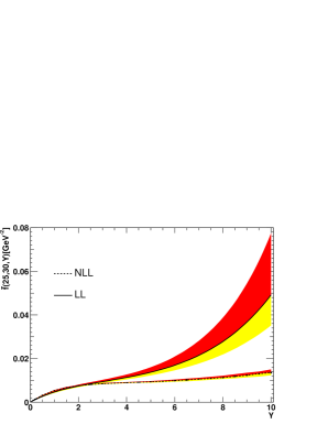
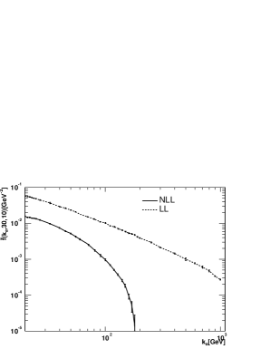
Figure 1: The NLL GGF: Evolution in rapidity at LL and NLL for $k_{a}=25$ GeV and $k_{b}=30$ GeV (left), and the dependence on $k_{a}$ for fixed $k_{b}=30$ GeV and $Y=10$ (right).

In $k_{t}$–space the NLL corrections are stable when the two transverse scales entering the forward GGF are similar. If they are very different then the convergence is not good, having an oscillatory behaviour with regions of negative values along the period of oscillation (see second plot of Fig. 1).

It is possible to improve the convergence of the expansion $\!{}^{{\bf?},{\bf?},{\bf?}}$. An original approach was suggested in $\!{}^{{\bf?}}$ based on the introduction of an all–orders resummation of terms compatible with renormalisation group evolution. In $\!{}^{{\bf?}}$ it has been shown how to apply this $RG$–resummation to the iterative solution here described. In a nutshell: For small $\bar{\alpha}_{s}$ the solution to the $\omega$–shift in $\!{}^{{\bf?}}$

$$\omega = {\bar{\alpha}}_{s}\left(1+\left({\rm a}+\frac{\pi^{2}}{6}\right){\bar{\alpha}}_{s}\right)\left(2\psi(1)-\psi\left(\gamma+\frac{\omega}{2}-{\rm b}\,{\bar{\alpha}}_{s}\right)-\psi\left(1-\gamma+\frac{\omega}{2}-{\rm b}\,{\bar{\alpha}}_{s}\right)\right)$$ (4)

$$+ {\bar{\alpha}}_{s}^{2}\left(\chi_{1}\left(\gamma\right)+\left(\frac{1}{2}\chi_{0}\left(\gamma\right)-{\rm b}\right)\left(\psi^{\prime}(\gamma)+\psi^{\prime}(1-\gamma)\right)-\left({\rm a}+\frac{\pi^{2}}{6}\right)\chi_{0}(\gamma)\right),$$

can be approximated by the sum of the solutions to the shift at each of the poles of the LL eigenvalue of the kernel, i.e.

$$\omega = \bar{\alpha}_{s}\chi_{0}(\gamma)+\bar{\alpha}_{s}^{2}\chi_{1}(\gamma)+\left\{\sum_{m=0}^{\infty}\left[\left(\sum_{n=0}^{\infty}\frac{(-1)^{n}(2n)!}{2^{n}n!(n+1)!}\frac{\left({\bar{\alpha}}_{s}+{\rm a}\,{\bar{\alpha}}_{s}^{2}\right)^{n+1}}{\left(\gamma+m-{\rm b}\,{\bar{\alpha}}_{s}\right)^{2n+1}}\right)\right.\right.$$ (5)

$$- \left.\left.\frac{\bar{\alpha}_{s}}{\gamma+m}-\bar{\alpha}_{s}^{2}\left(\frac{\rm a}{\gamma+m}+\frac{\rm b}{(\gamma+m)^{2}}-\frac{1}{2(\gamma+m)^{3}}\right)\right]+\left\{\gamma\rightarrow 1-\gamma\right\}\right\},$$

where $\chi_{0}$ and $\chi_{1}$ are the LL and NLL scale invariant parts of the kernel, and a and b the coefficients of the single and double poles in the collinear limit.

The numerical solution to Eq. (4) and expression (5) are compared in Fig. 2 (left).

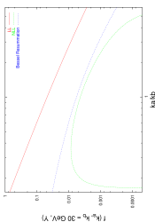
Figure 2: The LL and NLL scale invariant kernels together with the $RG$–improved kernel and the “all–poles” resummation (left). The collinear behaviour of the NLL GGF using the Bessel resummation (right).

The expansion is now stable in all regions with an intercept of 0.3 at NLL for $\bar{\alpha}_{s}=0.2$ (without running coupling effects). To implement Eq. (5) in $k_{t}$–space is simple $\!{}^{{\bf?}}$: Removing the term $-\frac{\bar{\alpha}_{s}^{2}}{4}\ln^{2}{\frac{q^{2}}{k^{2}}}$ from the real emission kernel, ${\cal K}_{r}\left(\vec{q},\vec{k}\right)$, and replacing it with

$$\left(\frac{q^{2}}{k^{2}}\right)^{-{\rm b}{\bar{\alpha}}_{s}\frac{\left|k-q\right|}{k-q}}\sqrt{\frac{2\left({\bar{\alpha}}_{s}+{\rm a}\,{\bar{\alpha}}_{s}^{2}\right)}{\ln^{2}{\frac{q^{2}}{k^{2}}}}}J_{1}\left(\sqrt{2\left({\bar{\alpha}}_{s}+{\rm a}\,{\bar{\alpha}}_{s}^{2}\right)\ln^{2}{\frac{q^{2}}{k^{2}}}}\right)-{\bar{\alpha}}_{s}-{\rm a}\,{\bar{\alpha}}_{s}^{2}+{\rm b}\,{\bar{\alpha}}_{s}^{2}\frac{\left|k-q\right|}{k-q}\ln{\frac{q^{2}}{k^{2}}},$$ (6)

with $J_{1}$ the Bessel function of the first kind. This prescription generates a convergent GGF as can be seen in Fig. 2 (right) where there are no oscillations, and can be immediately implemented in the iterative approach of $\!{}^{{\bf?}}$.

This iterative method integrates the phase space using a Monte Carlo sampling of different parton configurations. Multiplicities are extracted from the Poisson–like distribution in the number of iterations needed to reach convergence (Fig. 3 (left)). Azimuthal angular correlations can also be obtained (Fig. 3 (right)) $\!{}^{{\bf?}}$.

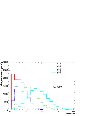
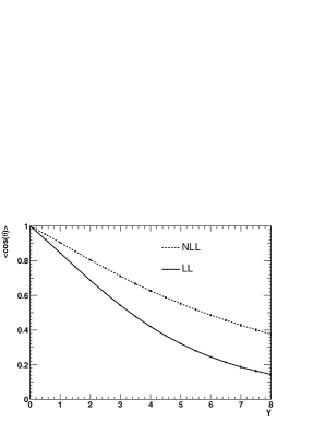
Figure 3: Distribution in the number of iterations and angular dependence of the NLL gluon Green’s function.

To show how the angular dependences are correctly described the NLL kernel in $N=4$ super Yang–Mills theory $\!{}^{{\bf?}}$ was studied in $\!{}^{{\bf?}}$. In particular, to calculate the contribution to the GGF from its Fourier components in the azimuthal angle one can extract the coefficients either using the kernel for different conformal spins as in $\!{}^{{\bf?}}$: $\sim\int d\gamma\left({\bf{k}_{a}^{2}}/{\bf{k}_{b}^{2}}\right)^{\gamma}\exp{(\omega_{n}(a,\gamma){\rm Y})}$, or using the iterative solution $\!{}^{{\bf?}}$: $\sim\int_{0}^{2\pi}{d\theta}\,f\left(\bf{k}_{a},\bf{k}_{b},{\rm Y}\right)\cos{\left(n\theta\right)}$. These two procedures match in their predictions and it can be seen that the $n=0$ Fourier component governs at large energies, decreasing the angular correlations.

The non–forward LL case was studied in $\!{}^{{\bf?}}$ and the same method applies at NLL. In $\!{}^{{\bf?}}$ it was shown how at large momentum transfer $t$ it is possible to study the diffusion into low and large scales of the transverse momenta in the gluon ladder. In particular, the diffusion into the infrared is cut off for finite values of $t$.

References

References

- [1] L. N. Lipatov, Sov. J. Nucl. Phys. 23, 338 (1976); V. S. Fadin, E. A. Kuraev and L. N. Lipatov, Phys. Lett. B 60, 50 (1975), Sov. Phys. JETP 44, 443 (1976), Sov. Phys. JETP 45, 199 (1977); I. I. Balitsky and L. N. Lipatov, Sov. J. Nucl. Phys. 28, 822 (1978), JETP Lett. 30, 355 (1979).
- [2] V. S. Fadin and L. N. Lipatov, Phys. Lett. B 429, 127 (1998); G. Camici and M. Ciafaloni, Phys. Lett. B 430, 349 (1998).
- [3] G. P. Salam, JHEP 9807, 019 (1998).
- [4] M. Ciafaloni, D. Colferai, G. P. Salam and A. M. Stasto, Phys. Lett. B 587 (2004) 87, Phys. Rev. D 68 (2003) 114003, Phys. Lett. B 576 (2003) 143, Phys. Lett. B 541 (2002) 314, Phys. Rev. D 66 (2002) 054014; M. Ciafaloni, D. Colferai and G. P. Salam, JHEP 0007 (2000) 054, JHEP 9910 (1999) 017, Phys. Rev. D 60 (1999) 114036; M. Ciafaloni and D. Colferai, Phys. Lett. B 452 (1999) 372.
- [5] L.N. Lipatov, JETP , 904 (1986); G. Camici and M. Ciafaloni, Phys. Lett. B , 118 (1997); D. A. Ross, Phys. Lett. B 431 (1998) 161; J. R. Forshaw, D. A. Ross and A. Sabio Vera, Phys. Lett. B 455 (1999) 273, Phys. Lett. B 498 (2001) 149; M. Ciafaloni, M. Taiuti and A. H. Mueller, Nucl. Phys. B 616 (2001) 349; Yu.V. Kovchegov and A.H. Mueller, Phys. Lett. B439 (1998) 423; N. Armesto, J. Bartels, M.A. Braun, Phys. Lett. B442 (1998) 459; S. J. Brodsky, V. S. Fadin, V. T. Kim, L. N. Lipatov and G. B. Pivovarov, JETP Lett. 70 (1999) 155; C. R. Schmidt, Phys. Rev. D 60 (1999) 074003; G. Chachamis, M. Lublinsky and A. Sabio Vera, Nucl. Phys. A 748 (2005) 649; G. Altarelli, R. D. Ball and S. Forte, Nucl. Phys. B 674 (2003) 459, Nucl. Phys. B 621 (2002) 359, Nucl. Phys. B 599 (2001) 383, Nucl. Phys. B 575 (2000) 313.
- [6] J. R. Andersen and A. Sabio Vera, Phys. Lett. B 567 (2003) 116.
- [7] J. R. Andersen and A. Sabio Vera, Nucl. Phys. B 679 (2004) 345.
- [8] A. Sabio Vera, Nucl. Phys. B 722 (2005) 65.
- [9] A. V. Kotikov and L. N. Lipatov, Nucl. Phys. B 582 (2000) 19.
- [10] J. R. Andersen and A. Sabio Vera, Nucl. Phys. B 699 (2004) 90.
- [11] J. R. Andersen and A. Sabio Vera, JHEP 0501 (2005) 045.