CPT-2004/P.081

The Dalitz decay $\pi^{0}\rightarrow e^{+}e^{-}\gamma$ revisited

Karol Kampf ^a,, Marc Knecht ^b, and Jiří Novotný ^a,

^aInstitute of Particle and Nuclear Physics, Charles University,
V Holesovickach 2, 180 00 Prague 8, Czech Republic

^bCentre de Physique Théorique, CNRS-Luminy, Case 907
F-13288 Marseille Cedex 9, France

The amplitude of the Dalitz decay $\pi^{0}\rightarrow e^{+}e^{-}\gamma$ is studied and its model-independent properties are discussed in detail. A calculation of radiative corrections is performed within the framework of two-flavour chiral perturbation theory, enlarged by virtual photons and leptons. The lowest meson dominance approximation, motivated by large $N_{C}$ considerations, is used for the description of the $\pi^{0}$-$\gamma^{*}$-$\gamma^{*}$ transition form factor and for the estimate of the NLO low energy constants involved in the analysis. The two photon reducible contributions is included and discussed. Previous calculations are extended to the whole kinematical range of the soft-photon approximation, thus allowing for the possibility to consider various experimental situations and observables.

1 Introduction

With a branching ratio of $(1.198\pm 0.032)\%$ [1], the three body decay $\pi^{0}\rightarrow e^{+}e^{-}\gamma$ is the second most important decay channel of the neutral pion. The dominant decay mode, $\pi^{0}\rightarrow\gamma\gamma$, with its overwhelming branching ratio of ($98.798\pm 0.032)\,\%$, is deeply connected to this three body decay. The other decay channels related to the anomalous $\pi^{0}$-$\gamma$-$\gamma$ vertex, like $\pi^{0}\rightarrow e^{+}e^{-}$ and $\pi^{0}\rightarrow e^{+}e^{-}e^{+}e^{-}$, are suppressed approximately by factors of $10^{-7}$ and $10^{-5}$, respectively. Another interest of the Dalitz decay lies in the fact that it provides information on the semi off-shell $\pi^{0}$-$\gamma$-$\gamma^{*}$ transition form factor ${\cal F}_{\pi^{0}\gamma\gamma^{*}}(q^{2})$ in the time-like region, and more specifically on its slope parameter $a_{\pi}$. The most recent determinations of $a_{\pi}$ obtained from measurements [4, 5, 6] of the differential decay rate of the Dalitz decay,

$$a_{\pi} = -0.11\pm 0.03\pm 0.08\quad{\cite[cite]{[\@@bibref{}{exp1}{}{}]}}$$

$$a_{\pi} = +0.026\pm 0.024\pm 0.0048\quad{\cite[cite]{[\@@bibref{}{exp2}{}{}]}}$$

$$a_{\pi} = +0.025\pm 0.014\pm 0.026\quad{\cite[cite]{[\@@bibref{}{exp3}{}{}]}},$$

are endowed with large error bars, as compared to the values extracted from the extrapolation of data at higher energies in the space-like region, $Q^{2}=-q^{2}>0.5$ GeV², obtained by CELLO [7] and CLEO [8],

$$a_{\pi} = +0.0326\pm 0.0026\pm 0.0026\quad{\cite[cite]{[\@@bibref{}{cello}{}{}]}}$$

$$a_{\pi} = +0.0303\pm 0.0008\pm 0.0009\pm 0.0012\quad{\cite[cite]{[\@@bibref{}{cleo}{}{}]}}$$

These extrapolations are however model dependent, and a direct and accurate determination of $a_{\pi}$ from the decay $\pi^{0}\rightarrow e^{+}e^{-}\gamma$ would offer a complementary source of information. Let us mention, in this context, the proposal [9] of the PrimEx experiment at TJNAF to study the reaction $e^{-}\gamma\to e^{-}\pi^{0}$, where the neutral pion is produced in the field of a nucleus through virtual photons from electron scattering [10]. Although this process concerns again virtualities in the space-like region, very low values of $Q^{2}$, in the range well below the lowest values attained by the CELLO experiment, can be achieved upon selecting the events according to the emission angles of the produced pion and of the scattered electron [10, 9].

On the theoretical side, several studies have addressed the issue of the radiative corrections to the decay $\pi^{0}\rightarrow e^{+}e^{-}\gamma$ in the past. At lowest order, the decay amplitude is of order ${\cal O}(e^{3})$. The next-to-leading radiative corrections to the total decay rate were first evaluated numerically by D. Joseph [11], with the result

$$\frac{\Gamma^{\text{rad}}(\pi^{0}\rightarrow e^{+}e^{-}\gamma)}{\Gamma(\pi^{0}\rightarrow\gamma\gamma)}\approx 1.0\times 10^{-4}.$$

This shows that the radiative contribution is tiny and can be neglected in the total decay rate. However, the differential decay rate, which provides the relevant observable for the determination of $a_{\pi}$, is sensitive to these radiative corrections. This problem was extensively studied in [12] and [13]. In all cases, the two-photon exchange terms were neglected, and some further approximations were made (e.g. restrictions in the kinematical region and on the energy of the bremsstrahlung photon). Subsequently, the Dalitz decay was further discussed in connection with the omission of the two photon exchange contributions. Particularly, during the 1980s, the controversial question of the actual size of these contributions was under debate, as well as the relevance of Low’s theorem in this context, cf. the articles quoted in [14]. Eventually, the non interchangeability of the limits of vanishing electron mass and photon momentum was identified [15] as the origin of the apparent puzzle raised by the contradictory results obtained previously by various authors.

Our purpose is to provide a complete treatment of the next-to-leading radiative corrections to the Dalitz decay, taking into account the theoretical progresses accomplished in various aspects related to this issue. For instance, in the studies quoted so far, the pion was taken as point-like. On the other hand, the leading order amplitude involves the form factor ${\cal F}_{\pi^{0}\gamma\gamma^{*}}(q^{2})$ with virtualities up to $q^{2}\sim M_{\pi^{0}}^{2}$, which is within the realm where chiral perturbation theory (ChPT) [16, 17, 18] is applicable. The details of the one-loop calculation of the $\pi^{0}$-$\gamma$-$\gamma^{*}$ vertex in ChPT can be found in [19]. However, we also need to consider (among other contributions) the electromagnetic corrections to ${\cal F}_{\pi^{0}\gamma\gamma^{*}}(q^{2})$. We are thus led to reformulate and extend the results described above within the unified and self-contained framework of ChPT with virtual photons, as it was formulated in [20] and in [21]. Actually, it is also quite straightforward to include light leptons in the effective theory, as described in [22], or, in the context of semileptonic decays of the light mesons, in [23]. Throughout, we shall work within the framework of two light quark flavours, $u$ and $d$. The corresponding extension to virtual photons is to be found in Refs. [24] and [25]. However, contributions of next-to-leading order ${\cal O}(e^{5})$ to the amplitude now involve the doubly off-shell $\pi^{0}$-$\gamma^{*}$-$\gamma^{*}$ transition form factor ${\cal A}_{\pi^{0}\gamma^{*}\gamma^{*}}(q_{1}^{2},q_{2}^{2})$, but for arbitrarily large virtualities, a situation which cannot be dealt with within ChPT. We shall introduce and use a representation [26, 27] of the form factor ${\cal A}_{\pi^{0}\gamma^{*}\gamma^{*}}(q_{1}^{2},q_{2}^{2})$ that relies on properties of both the large-$N_{C}$ limit and the short-distance regime of QCD. The same framework also allows us to supplement our analysis with estimates of the relevant low energy constants, along the lines of, for instance, Refs. [28] and [27].

The material of this article is organized as follows. The general properties (kinematics, diagram topologies,…) of the amplitude are discussed in Section 2. Section 3 is devoted to the computation of the differential decay rate at next-to-leading order (NLO). Numerical results are presented in Section 4. A brief summary and conclusions are gathered in Section 5. For reasons of convenience, various technical details have been included in the form of appendices. Preliminary reports of the present work have appeared in Refs. [29, 30].

2 General properties of the Dalitz decay amplitude

In this section we describe the general structure of the amplitude for the Dalitz decay $\pi^{0}\rightarrow e^{+}e^{-}\gamma$, relevant for the discussion of the contributions both at leading order, ${\cal O}(e^{3})$, and at next-to-leading order, ${\cal O}(e^{5})$.

2.1 Notation and kinematics

The Dalitz decay amplitude $\mathcal{M}_{\pi^{0}\rightarrow e^{+}e^{-}\gamma}$ is defined as

$$\langle e^{+}(p_{+},s_{+})e^{-}(p_{-},s_{-})\gamma(k,\lambda);\,{out}|\pi^{0}(P);\,{in}\rangle=i(2\pi)^{4}\delta^{(4)}(P-p_{+}-p_{-}-k)\mathcal{M}_{\pi^{0}\rightarrow e^{+}e^{-}\gamma},$$ (2.1)

where the transition matrix element has to be evaluated in the presence of the strong and the electromagnetic interactions. Lorentz covariance allows to express the amplitude $\mathcal{M}_{\pi^{0}\rightarrow e^{+}e^{-}\gamma}$ in the form

$$\mathcal{M}_{\pi^{0}\rightarrow e^{+}e^{-}\gamma}=\bar{u}(p_{-},s_{-})\Gamma_{\mu}(p_{+},p_{-},k)v(p_{+},s_{+})\varepsilon^{*\mu}(k),$$ (2.2)

with

$$\bar{u}(p_{-},s_{-})\Gamma_{\mu}(p_{+},p_{-},k)v(p_{+},s_{+})=\lim_{k^{2}\to 0}\,ie\langle e^{+}(p_{+},s_{+})e^{-}(p_{-},s_{-});\,{out}|j_{\mu}(0)|\pi^{0}(P);\,{in}\rangle$$ (2.3)

given in terms of the electromagnetic current

$$j_{\mu}=\frac{2}{3}\bar{u}\gamma_{\mu}u-\frac{1}{3}\bar{d}\gamma_{\mu}d-{\bar{\psi_{e}}}\gamma_{\mu}\psi_{e}+\ldots$$ (2.4)

Invariance under parity, charge conjugation, and gauge symmetry,

$$k^{\mu}\bar{u}(p_{-},s_{-})\Gamma_{\mu}(p_{+},p_{-},k)v(p_{+},s_{+})=0,$$ (2.5)

implies a transverse structure and a decomposition in terms of four independent form factors

$$\Gamma^{\mu}(p_{+},p_{-},k) =\phantom{+}P(x,y)[(k\cdot p_{+})p_{-}^{\mu}-(k\cdot p_{-})p_{+}^{\mu}]\gamma_{5}$$

$$\phantom{=}\;+A_{+}(x,y)[\not{k}\,p_{+}^{\mu}-(k\cdot p_{+})\gamma^{\mu}]\gamma_{5}-A_{-}(x,y)[\not{k}\,p_{-}^{\mu}-(k\cdot p_{-})\gamma^{\mu}]\gamma_{5}$$

$$\phantom{=}\;-\mathrm{i}T(x,y)\sigma^{\mu\nu}k_{\nu}\gamma_{5}.$$ (2.6)

The invariant form factors $P(x,y)$, $A_{\pm}(x,y)$ and $T(x,y)$ are functions of two independent kinematical variables, which we have chosen as ($m$ denotes the electron mass, $p_{-}^{2}=p_{+}^{2}=m^{2}$)

$$x = \frac{(p_{+}+p_{-})^{2}}{M_{\pi^{0}}^{2}},\qquad\nu^{2}\leq x\leq 1,\qquad\nu^{2}\,=\frac{4m^{2}}{M_{\pi^{0}}^{2}},$$

$$y = \frac{2P\cdot(p_{+}-p_{-})}{M_{\pi^{0}}^{2}(1-x)},\,\,\,\,-\sigma_{e}(M_{\pi^{0}}^{2}x)\leq y\leq\sigma_{e}(M_{\pi^{0}}^{2}x),\quad\sigma_{e}(s)=\sqrt{1-\frac{4m^{2}}{s}}.$$

In the pion rest frame, these invariants can be expressed in terms of the energies of the photon ($\omega$), of the positron ($E_{+}$) and of the electron ($E_{-}$) as

$$1-x = 2\,\frac{\omega}{M_{\pi^{0}}},$$

$$y = \frac{E_{+}-E_{-}}{\omega}.$$

In terms of the variables $x$ and $y$, charge conjugation invariance implies that the form factors satisfy the symmetry relations

$$P(x,y)=P(x,-y),\ A_{\mp}(x,y)=A_{\pm}(x,-y),\ T(x,y)=T(x,-y).$$

Let us note that the form factors $P(x,y)$, $A_{\pm}(x,y)$ and $T(x,y)$ can be projected out from $\Gamma^{\mu}$ by means of the formula

$$F=\mathrm{Tr}\bigl{(}\Lambda_{F}^{\mu}(\not{p}_{-}+m)\Gamma_{\mu}(\not{p}_{+}-m)\bigr{)},$$ (2.7)

where $\Lambda_{F}^{\mu}$, with $F=P$, $A_{\pm}$ , $T$, are projectors satisfying $k\cdot\Lambda_{F}=0$. Explicit expressions of these projectors are given in Appendix A.

In terms of the variables $x$, $y$, the differential decay rate is given by the formula

$$\mathrm{d}\Gamma=\frac{1}{(2\pi)^{3}}\frac{M_{\pi^{0}}}{64}(1-x)\overline{|\mathcal{M}_{\pi^{0}\rightarrow e^{+}e^{-}\gamma}|^{2}}\,\mathrm{d}x\mathrm{d}y.$$ (2.8)

Expressed in terms of the form factors $P$, $A_{\pm}$ and $T$, the square of the invariant amplitude (summed over polarizations) reads

$$\overline{|\mathcal{M}_{\pi^{0}\rightarrow e^{+}e^{-}\gamma}|^{2}} =\sum_{\mathrm{polarizations}}|\mathcal{M}_{\pi^{0}\rightarrow e^{+}e^{-}\gamma}|^{2}=\frac{1}{8}\,M_{\pi^{0}}^{4}(1-x)^{2}$$

$$\phantom{=}\;\times\bigl{\{}[M_{\pi^{0}}^{2}x(1-y^{2})-4m^{2}][|P|^{2}xM_{\pi^{0}}^{2}-2mP(A_{+}+A_{-})^{*}$$

$$\phantom{=\times}\;\;-2mP^{*}(A_{+}+A_{-})+2PT^{*}+2P^{*}T]$$

$$\phantom{=\times}\;\;+2(xM_{\pi^{0}}^{2}-4m^{2})[|A_{+}|^{2}(1+y)^{2}+|A_{-}|^{2}(1-y)^{2}]$$

$$\phantom{=\times}\;\;-8m^{2}y^{2}(A_{+}^{*}A_{-}+A_{+}A_{-}^{*})+8my(1+y)(A_{+}^{*}T+A_{+}T^{*})$$

$$\phantom{=\times}\;\;-8my(1-y)(A_{-}^{*}T+A_{-}T^{*})+8(1-y^{2})|T|^{2}\bigr{\}}.$$ (2.9)

In the case $m=0$, this reduces to

$$\overline{|\mathcal{M}_{\pi^{0}\rightarrow e^{+}e^{-}\gamma}|^{2}}=\frac{1}{8}\,M_{\pi^{0}}^{4}(1-x)^{2}\bigl{\{}M_{\pi^{0}}^{2}x(1-y^{2})[|P|^{2}xM_{\pi^{0}}^{2}+2PT^{*}+2P^{*}T]\\ +2M_{\pi^{0}}^{2}x[|A_{+}|^{2}(1+y^{2})+|A_{-}|^{2}(1-y^{2})]+8(1-y^{2})|T|^{2}\bigr{\}}.$$

As usual, higher order corrections induced by virtual photon contributions generate infrared singularities, even for a nonvanishing electron mass $m$. In order to obtain an infrared finite and physically observable (differential) decay rate, the emission processes of real soft photons have also to be considered.

2.2 Anatomy of the Dalitz decay amplitude

The contributions to the amplitude $\mathcal{M}_{\pi^{0}\rightarrow e^{+}e^{-}\gamma}$ rather naturally separate into two main classes. The first one corresponds to the Feynman graphs where the electron-positron pair is produced by a single photon (Dalitz pair). The leading contribution, of order ${\cal O}(e^{3})$, to the decay amplitude belongs to these one-photon reducible graphs. They involve the semi-off-shell $\pi^{0}$-$\gamma$-$\gamma^{*}$ vertex ${\cal F}_{\pi^{0}\gamma\gamma^{*}}(q^{2})$, see Fig. 1. The second class of contributions corresponds to the one-photon irreducible topologies. They can be further separated into the one-fermion reducible contributions, which represent the radiative corrections to the $\pi^{0}\rightarrow e^{+}e^{-}$ process (see Fig. 2), and the remaining one-particle irreducible graphs (Fig. 3), starting with the two photon exchange box diagram, see the second graph on Fig. 4. Both types of these one-photon irreducible contributions to the amplitude involve the doubly off-shell $\pi^{0}$-$\gamma^{*}$-$\gamma^{*}$ vertex ${\cal A}_{\pi^{0}\gamma^{*}\gamma^{*}}(q_{1}^{2},q_{2}^{2})$. They are suppressed with respect to the lowest order one-photon reducible contribution, starting at the order ${\cal O}(e^{5})$ with the contributions depicted on Fig. 4. Let us now discuss consecutively these different topologies in greater detail.

2.2.1 The one-photon reducible contributions

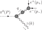
Figure 1: One-photon reducible diagrams

The one-photon reducible topologies are shown on Fig. 1. They contain the leading order contribution to $\mathcal{M}_{\pi^{0}\rightarrow e^{+}e^{-}\gamma}$, and involve only low virtualities of the semi off-shell form factor ${\cal F}_{\pi^{0}\gamma\gamma^{*}}(q^{2})$. The contribution at leading, ${\cal O}(e^{3})$, but also at next-to-leading, ${\cal O}(e^{5})$, orders can thus be fully treated within the framework of ChPT, extended to virtual photons. The general expression for this one-photon reducible part of the Dalitz decay amplitude has the form

$$\mathcal{M}_{\pi^{0}\rightarrow e^{+}e^{-}\gamma}^{1\gamma R}=\bar{u}\Gamma_{\mu}^{1\gamma R}(p_{+},p_{-},k)v\varepsilon^{*\mu}(k),$$

where

$$\Gamma^{1\gamma R}_{\mu}(p_{+},p_{-},k)=+\mathrm{i}e^{2}\varepsilon_{\mu}^{\ \nu\alpha\beta}q_{\alpha}k_{\beta}\,\mathcal{F}_{\pi^{0}\gamma\gamma^{*}}(q^{2})\,\mathrm{i}D_{\nu\rho}^{T}(q)(-\mathrm{i}e)\Lambda^{\rho}(p_{-},-p_{+}).$$

In this and the following expressions, $q=p_{+}+p_{-}$. The form factor $\mathcal{F}_{\pi^{0}\gamma\gamma^{*}}(q^{2})$ is related to the doubly off-shell form factor $\mathcal{A}_{\pi^{0}\gamma^{*}\gamma^{*}}(q_{1}^{2},q_{2}^{2})$, defined as

$$\int d^{4}x\,e^{il\cdot x}\langle 0|T(j^{\mu}(x)j^{\nu}(0)|\pi^{0}(P)\rangle=-\mathrm{i}\varepsilon^{\mu\nu\alpha\beta}l_{\alpha}P_{\beta}\,\mathcal{A}_{\pi^{0}\gamma^{*}\gamma^{*}}(l^{2},(P-l)^{2}),$$ (2.10)

by

$$\mathcal{F}_{\pi^{0}\gamma\gamma^{*}}(q^{2})=\mathcal{A}_{\pi^{0}\gamma^{*}\gamma^{*}}(0,q^{2}).$$

Here the matrix element on the left hand side can be obtained by means of the LSZ formula from the three point Green’s function $\langle VVA\rangle$, calculated within QCD+QED (i.e. with the QED corrections included). Furthermore, $D_{\mu\nu}^{T}(q)$ is the transverse part of the photon propagator (the longitudinal, gauge dependent, part of the photon propagator does not contribute),

$$\mathrm{i}D_{\mu\nu}^{T}(q)=-\mathrm{i}\,\frac{g_{\mu\nu}-q_{\mu}q_{\nu}/q^{2}}{q^{2}[1+\overline{\Pi}(q^{2})]}\,,$$

where $\overline{\Pi}(q^{2})$ is the renormalized vacuum polarization function (in the on-shell renormalization scheme with $\overline{\Pi}(0)=0$), and $\Lambda^{\rho}(q_{1},q_{2})$ stands for the off-shell one-particle irreducible $e^{+}$-$e^{-}$-$\gamma$ vertex function. For on-shell momenta, $q_{1}=p_{-}$, $q_{2}=-p_{+}$, it can be decomposed in terms of the Dirac and Pauli form factors $\overline{F}_{1,2}(q^{2})$,

$$\bar{u}\Lambda^{\mu}(p_{-},-p_{+})v=\bar{u}[\overline{F}_{1}(q^{2})\gamma^{\mu}+\frac{1}{2m}\overline{F}_{2}(q^{2})\mathrm{i}\sigma^{\mu\nu}q_{\nu}]v,$$

with $\overline{F}_{1}(0)=1$ and $\overline{F}_{2}(0)=a_{e}$, where $a_{e}$ is the anomalous magnetic moment of the electron.

Note that the one-photon reducible part $\Gamma_{\mu}^{1\gamma R}(p_{+},p_{-},k)$ is gauge invariant by itself,

$$k^{\mu}\Gamma_{\mu}^{1\gamma R}(p_{+},p_{-},k)=0,$$

and therefore it can be expressed in terms of form factors $P$, $A_{\pm}$, $T$. Using e.g. the formulae (2.7), (A.1), (A.2), and (A.3), one obtains

$$P^{1\gamma R}(x,y) =-e^{3}\mathcal{F}_{\pi^{0}\gamma\gamma^{*}}(xM_{\pi^{0}}^{2})\frac{1}{xM_{\pi^{0}}^{2}[1+\overline{\Pi}(xM_{\pi^{0}}^{2})]}\frac{\mathrm{i}}{m}\,\overline{F}_{2}(xM_{\pi^{0}}^{2}),$$

$$A^{1\gamma R}_{\pm}(x,y) =e^{3}\mathcal{F}_{\pi^{0}\gamma\gamma^{*}}(xM_{\pi^{0}}^{2})\frac{1}{xM_{\pi^{0}}^{2}[1+\overline{\Pi}(xM_{\pi^{0}}^{2})]}\mathrm{i}\overline{F}_{1}(xM_{\pi^{0}}^{2}),$$ (2.11)

$$T^{1\gamma R}(x,y) =e^{3}\mathcal{F}_{\pi^{0}\gamma\gamma^{*}}(xM_{\pi^{0}}^{2})\frac{1}{xM_{\pi^{0}}^{2}[1+\overline{\Pi}(xM_{\pi^{0}}^{2})]}\mathrm{i}\bigl{[}2m\overline{F}_{1}(xM_{\pi^{0}}^{2})+\frac{xM_{\pi^{0}}^{2}}{2m}\,\overline{F}_{2}(xM_{\pi^{0}}^{2})\bigr{]}.$$

2.2.2 One-fermion reducible and one-particle irreducible contributions

The one-fermion reducible and the one-particle irreducible topologies, shown on Fig. 2 and on Fig. 3, respectively, both start at order ${\cal O}(e^{5})$.

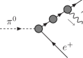
Figure 2: One-fermion reducible diagrams

Since the one-photon reducible part $\mathcal{M}_{\pi^{0}\rightarrow e^{+}e^{-}\gamma}^{1\gamma R}$ of the invariant amplitude is transverse by itself, the one-fermion reducible and one particle irreducible contributions $\mathcal{M}_{\pi^{0}\rightarrow e^{+}e^{-}\gamma}^{1\psi R}+\mathcal{M}_{\pi^{0}\rightarrow e^{+}e^{-}\gamma}^{1PI}$ together also represent a transverse subset. However, these two types of contributions are not transverse when taken separately.

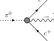
Figure 3: One-particle irreducible diagrams

Let us first concentrate on the one-fermion reducible topology. These contributions can be expressed in the form

$$\mathcal{M}_{\pi^{0}\rightarrow e^{+}e^{-}\gamma}^{1\psi R}=\overline{u}\Gamma_{\mu}^{1\psi R}(p_{+},p_{-},k)v\varepsilon^{\mu}(k)^{*},$$

where

$$\mathrm{i}\Gamma_{\mu}^{1\psi R}(p_{+},p_{-},k)=(-\mathrm{i}e)\Lambda_{\mu}(p_{-},p_{-}+k)\mathrm{i}S(p_{-}+k)\mathrm{i}\Gamma_{\pi^{0}e^{-}e^{+}}(p_{-}+k,p_{+})\\ \phantom{=}+\mathrm{i}\Gamma_{\pi^{0}e^{-}e^{+}}(p_{-},p_{+}+k)\mathrm{i}S(-p_{+}-k)(-\mathrm{i}e)\Lambda_{\mu}(-p_{+}-k,-p_{+}).$$ (2.12)

In this formula,

$$\mathrm{i}S(q)=\frac{\mathrm{i}}{\not{q}-m-\Sigma(q)}$$

is the full fermion propagator, with

$$\Sigma(q)=\not{q}\,\Sigma_{V}(q^{2})+\Sigma_{S}(q^{2})$$ (2.13)

the fermion self-energy, while $\Lambda_{\mu}(q_{1},q_{2})=\gamma_{\mu}+{\cal O}(\alpha)$ and $\Gamma_{\pi^{0}e^{-}e^{+}}(q_{1},q_{2})$ are the (off-shell) one-particle irreducible $e^{+}$-$e^{-}$-$\gamma$ and $\pi^{0}$-$e^{-}$-$e^{+}$ vertices, respectively. As we have already mentioned, $\mathrm{i}\Gamma_{\mu}^{1\psi R}(p_{+},p_{-},k)$ is not transverse, since $\Lambda_{\mu}(q_{1},q_{2})$ satisfies the Ward-Takahashi identity

$$(q_{1}-q_{2})\cdot\Lambda(q_{1},q_{2})=S^{-1}(q_{1})-S^{-1}(q_{2}).$$ (2.14)

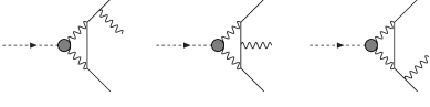
Figure 4: One-photon irreducible contributions at one-loop level.

The solution of this identity reads

$$\Lambda_{\mu}(q_{1},q_{2})=\Lambda_{\mu}^{L}(q_{1},q_{2})+\Lambda_{\mu}^{T}(q_{1},q_{2}),$$ (2.15)

with

$$(q_{1}-q_{2})\cdot\Lambda^{T}(q_{1},q_{2})=0,$$ (2.16)

and the longitudinal part, which consists of any particular solution of Eq. (2.14), may conveniently be chosen [31] as

$$\Lambda_{\mu}^{L}(q_{1},q_{2}) = \frac{1}{2}(\not{q}_{1}+\not{q}_{2})(q_{1}+q_{2})_{\mu}\,\frac{\Sigma_{V}(q_{2}^{2})-\Sigma_{V}(q_{1}^{2})}{q_{1}^{2}-q_{2}^{2}}$$ (2.17)

$$\quad+\gamma_{\mu}\Bigl{[}1-\frac{1}{2}\Sigma_{V}(q_{2}^{2})-\frac{1}{2}\Sigma_{V}(q_{1}^{2})\Bigr{]}+(q_{1}+q_{2})_{\mu}\,\frac{\Sigma_{S}(q_{2}^{2})-\Sigma_{S}(q_{1}^{2})}{q_{1}^{2}-q_{2}^{2}}.$$

The transverse part $\Lambda_{\mu}^{T}(q_{1},q_{2})$ is then parameterized in terms of eight form factors $A_{i}$, $i=1,\ldots,8$, corresponding to the eight available independent transverse tensor structures $T_{\mu}^{i}$, $i=1,\ldots,8$ (we will not reproduce them here, for a detailed discussion and explicit expressions, see Refs. [31] and [32])

$$\Lambda_{\mu}^{T}(q_{1},q_{2})=\sum_{i=1}^{8}A_{i}(q_{1}^{2},q_{2}^{2},(q_{1}-q_{2})^{2})T_{\mu}^{i}(q_{1},q_{2}).$$ (2.18)

The decomposition (2.15) of the vertex function $\Lambda(q_{1},q_{2})$ induces the corresponding decomposition of $\Gamma_{\mu}^{1\psi R}(p_{+},p_{-},k)$,

$$\Gamma_{\mu}^{1\psi R}(p_{+},p_{-},k)=\Gamma_{\mu}^{1\psi R;T}(p_{+},p_{-},k)+\Gamma_{\mu}^{1\psi R;L}(p_{+},p_{-},k),$$ (2.19)

with

$$k^{\mu}\Gamma_{\mu}^{1\psi R;T}(p_{+},p_{-},k)=0$$ (2.20)

and

$$k^{\mu}\Gamma_{\mu}^{1\psi R;L}(p_{+},p_{-},k) = e\Gamma_{\pi^{0}e^{-}e^{+}}(p_{-}+k,p_{+})-e\Gamma_{\pi^{0}e^{-}e^{+}}(p_{-},p_{+}+k)$$ (2.21)

$$-S^{-1}(p_{-})S(p_{-}+k)e\Gamma_{\pi^{0}e^{-}e^{+}}(p_{-}+k,p_{+})$$

$$+e\Gamma_{\pi^{0}e^{-}e^{+}}(p_{-},p_{+}+k)S(-p_{+}-k)S^{-1}(-p_{+}).$$

Therefore

$$\overline{u}\,k\cdot\Gamma^{1\psi R;L}(p_{+},p_{-},k)v=e\overline{u}[\Gamma_{\pi^{0}e^{-}e^{+}}(p_{-}+k,p_{+})-\Gamma_{\pi^{0}e^{-}e^{+}}(p_{-},p_{+}+k)]v.$$ (2.22)

This non transverse piece should be cancelled by the contribution $\overline{u}(k\cdot\Gamma^{1PI})v$ of the one-particle irreducible graphs. In addition, the transverse part $\Gamma_{\mu}^{1\psi R;T}(p_{+},p_{-},k)$ admits a representation of the type (2.6), with appropriate form factors $F^{1\psi R;T}(x,y)$, $A_{\pm}^{1\psi R;T}(x,y)$, and $T^{1\psi R;T}(x,y)$, up to possible terms proportional to $k_{\mu}$, which cancel when contracted with $\varepsilon^{\mu}(k)^{*}$.

As for the vertex $\Gamma_{\pi^{0}e^{-}e^{+}}(q_{2},q_{1})$, it can be decomposed (using Lorentz invariance, the Dirac structure of the inverse fermion propagator $S^{-1}(q)$, and charge conjugation invariance) as

$$\Gamma_{\pi^{0}e^{-}e^{+}}(q_{2},q_{1})=P_{\pi^{0}e^{-}e^{+}}(q_{2}^{2},q_{1}^{2})\gamma_{5}+\gamma_{5}S^{-1}(-q_{1})A_{\pi^{0}e^{-}e^{+}}(q_{2}^{2},q_{1}^{2})\\ +S^{-1}(q_{2})\gamma_{5}A_{\pi^{0}e^{-}e^{+}}(q_{1}^{2},q_{2}^{2})+S^{-1}(q_{2})\gamma_{5}S^{-1}(-q_{1})T_{\pi^{0}e^{-}e^{+}}(q_{2}^{2},q_{1}^{2}),$$ (2.23)

where $P_{\pi^{0}e^{-}e^{+}}$, $A_{\pi^{0}e^{-}e^{+}}$, and $T_{\pi^{0}e^{-}e^{+}}$ are scalar form factors, which, as a consequence of charge conjugation invariance, satisfy the additional relations

$$P_{\pi^{0}e^{-}e^{+}}(q_{2}^{2},q_{1}^{2})=P_{\pi^{0}e^{-}e^{+}}(q_{1}^{2},q_{2}^{2}),\ T_{\pi^{0}e^{-}e^{+}}(q_{2}^{2},q_{1}^{2})=T_{\pi^{0}e^{-}e^{+}}(q_{1}^{2},q_{2}^{2}).$$ (2.24)

The form factor $P_{\pi^{0}e^{-}e^{+}}$ is then related to the on-shell $\pi^{0}\rightarrow e^{+}e^{-}$ amplitude,

$$\mathcal{M}_{\pi^{0}\rightarrow e^{+}e^{-}}=\overline{u}(p_{-},s_{-})\gamma_{5}v(p_{+},s_{+})P_{\pi^{0}e^{-}e^{+}}(m^{2},m^{2}).$$

In terms of the form factors (2.23) we can write

$$\mathcal{M}_{\pi^{0}\rightarrow e^{+}e^{-}\gamma}^{1\psi R} = e\,\varepsilon^{\mu}(k)^{*}\overline{u}\bigl{\{}\Lambda_{\mu}(p_{-},p_{-}+k)S(p_{-}+k)P_{\pi^{0}e^{-}e^{+}}(m^{2}+2(k\cdot p_{-}),m^{2})\gamma_{5}$$ (2.25)

$$\;+P_{\pi^{0}e^{-}e^{+}}(m^{2},m^{2}+2(k\cdot p_{+}))\gamma_{5}S(-p_{+}-k))\Lambda_{\mu}(-p_{+}-k,-p_{+})$$

$$\;+\Lambda_{\mu}(p_{-},p_{-}+k)\gamma_{5}A_{\pi^{0}e^{-}e^{+}}(m^{2},m^{2}+2(k\cdot p_{-}))$$

$$\;+\gamma_{5}\Lambda_{\mu}(-p_{+}-k,-p_{+})A_{\pi^{0}e^{-}e^{+}}(m^{2},m^{2}+2(k\cdot p_{+}))\bigr{\}}v.$$

At leading order in the fine structure constant $\alpha$, $\Gamma_{\pi^{0}e^{+}e^{-}}$ is given by

$$\Gamma_{\pi^{0}e^{-}e^{+}}(q_{2},q_{1}) = -e^{4}\varepsilon^{\mu\nu\alpha\beta}\int\frac{\mathrm{d}^{4}l}{(2\pi)^{4}}\,\mathcal{A}_{\pi^{0}\gamma^{*}\gamma^{*}}(l^{2},(q_{1}+q_{2}-l)^{2})$$ (2.26)

$$\times\frac{l_{\alpha}(q_{1}+q_{2})_{\beta}}{(l^{2}+i0)[(q_{1}+q_{2}-l)^{2}+i0]}\,\gamma_{\mu}\,\frac{\mathrm{i}}{\not{q}_{2}-\not{l}-m+i0}\,\gamma_{\nu}\,,$$

where $\mathcal{A}_{\pi^{0}\gamma^{*}\gamma^{*}}(q_{1}^{2},q_{2}^{2})$ is now restricted to its pure QCD part. The corresponding expression of $\Gamma_{\mu}^{1\psi R}(p_{+},p_{-},k)$ then reads

$$\mathrm{i}\Gamma_{\mu}^{1\psi R}(p_{+},p_{-},k) = e^{5}\varepsilon^{\rho\sigma\alpha\beta}\int\frac{\mathrm{d}^{4}l}{(2\pi)^{4}}\,\mathcal{A}_{\pi^{0}\gamma^{*}\gamma^{*}}(l^{2},(P-l)^{2})\,\frac{l_{\alpha}P_{\beta}}{(l^{2}+\mathrm{i}0)[(P-l)^{2}+\mathrm{i}0]}$$ (2.27)

$$\times\bigg{[}\gamma_{\mu}\,\frac{\mathrm{i}}{\not{p}_{-}+\not{k}-m+\mathrm{i}0}\,\gamma_{\rho}\,\frac{\mathrm{i}}{\not{p}_{-}+\not{k}-\not{l}-m+\mathrm{i}0}\,\gamma_{\sigma}$$

$$\ -\gamma_{\rho}\,\frac{\mathrm{i}}{\not{p}_{-}-\not{l}-m+\mathrm{i}0}\,\gamma_{\sigma}\,\frac{\mathrm{i}}{\not{p}_{+}+\not{k}+m+\mathrm{i}0}\,\gamma_{\mu}\bigg{]}.$$

The general properties of the form factor $\mathcal{A}_{\pi^{0}\gamma^{*}\gamma^{*}}(q_{1}^{2},q_{2}^{2})$ are summarized in Appendix B. Here we only note that the short distance behaviour of $\mathcal{A}_{\pi^{0}\gamma^{*}\gamma^{*}}(l^{2},(P-l)^{2})$ in QCD makes it act as an ultraviolet cut-off, so that the loop integral on the right-hand side of (2.26) actually converges.

Finally, the one-particle irreducible part of the amplitude

$$\mathcal{M}_{\pi^{0}\rightarrow e^{+}e^{-}\gamma}^{1PI}=\overline{u}\Gamma_{\mu}^{1PI}(p_{+},p_{-},k)v\varepsilon^{\mu}(k)^{*}$$

starts at the order $e^{5}$ with the box diagram of Fig. 4,

$$\mathrm{i}\Gamma_{\mu}^{1PI}(p_{+},p_{-},k) = e^{5}\varepsilon^{\rho\sigma\alpha\beta}\int\frac{\mathrm{d}^{4}l}{(2\pi)^{4}}\,\mathcal{A}_{\pi^{0}\gamma^{*}\gamma^{*}}(l^{2},(P-l)^{2})\,\frac{l_{\alpha}P_{\beta}}{(l^{2}+\mathrm{i}0)[(P-l)^{2}+\mathrm{i}0]}$$ (2.28)

$$\times\gamma_{\rho}\,\frac{\mathrm{i}}{\not{p}_{-}-\not{l}-m+\mathrm{i}0}\,\gamma_{\mu}\,\frac{\mathrm{i}}{\not{p}_{-}+\not{k}-\not{l}-m+\mathrm{i}0}\,\gamma_{\sigma},$$

which is also ultraviolet finite. At this order, one verifies that the sum $\overline{u}\Gamma_{\mu}^{1\psi R}(p_{+},p_{-},k)v+\overline{u}\Gamma_{\mu}^{1PI}(p_{+},p_{-},k)v$ is indeed transverse.

3 The NLO differential decay rate

The leading order amplitude corresponds to the ${\cal O}(e^{3})$ one-photon reducible contribution, evaluated at lowest order in the extended chiral expansion, i.e. with $\overline{F}_{1}(q^{2})=1$, $\overline{F}_{2}(q^{2})=\overline{\Pi}(q^{2})=0$, and with the form factor $\mathcal{A}_{\pi^{0}\gamma^{*}\gamma^{*}}(l^{2},(P-l)^{2})$ reduced to its expression for a pointlike pion, i.e. a constant, $\mathcal{A}_{\pi^{0}\gamma^{*}\gamma^{*}}^{LO}=-N_{C}/12\pi^{2}F_{\pi}$, fixed by the chiral anomaly. The leading order expressions of the form factors $P$, $A_{\pm}$ and $T$ are then given, for $N_{C}=3$ and according to Eq. (2.11), by

$$P^{LO}(x,y) = 0,$$

$$A_{\pm}^{LO}(x,y) = -\frac{\mathrm{i}e^{3}}{4\pi^{2}F_{\pi}M_{\pi^{0}}^{2}}\cdot\frac{1}{x},$$

$$T^{LO}(x,y) = -\frac{2\mathrm{i}me^{3}}{4\pi^{2}F_{\pi}M_{\pi^{0}}^{2}}\cdot\frac{1}{x}.$$ (3.1)

Note that in the limit $m\rightarrow 0$, only the form factors $A_{\pm}^{LO}$ survive. The square of the leading invariant amplitude summed over polarizations is, according to (2.9),

$$\overline{|\mathcal{M}_{\pi^{0}\rightarrow e^{+}e^{-}\gamma}^{LO}|^{2}}=\frac{1}{32}\frac{e^{6}}{\pi^{4}F_{\pi}^{2}}\,\frac{(1-x)^{2}}{x^{2}}\,[M_{\pi^{0}}^{2}x(1+y^{2})+4m^{2}]$$ (3.2)

and the corresponding partial decay rates read

$$\frac{\mathrm{d}\Gamma^{LO}}{\mathrm{d}x\mathrm{d}y} =\frac{\alpha^{3}}{(4\pi)^{4}}\frac{M_{\pi^{0}}}{F_{\pi}^{2}}\,\frac{(1-x)^{3}}{x^{2}}\,[M_{\pi^{0}}^{2}x(1+y^{2})+4m^{2}],$$

$$\frac{\mathrm{d}\Gamma^{LO}}{\mathrm{d}x} =\frac{\alpha^{3}}{(4\pi)^{4}}\frac{8}{3}\frac{M_{\pi^{0}}}{F_{\pi}^{2}}\,\frac{(1-x)^{3}}{x^{2}}\,\sigma_{e}(xM_{\pi^{0}}^{2})\,(xM_{\pi^{0}}^{2}+2m^{2}).$$ (3.3)

The next-to-leading corrections to the differential decay rates will be described as

$$\begin{split}\frac{\mathrm{d}\Gamma}{\mathrm{d}x\mathrm{d}y}&=\delta(x,y)\,\frac{\mathrm{d}\Gamma^{LO}}{\mathrm{d}x\mathrm{d}y},\\ \frac{\mathrm{d}\Gamma}{\mathrm{d}x}&=\delta(x)\,\frac{\mathrm{d}\Gamma^{LO}}{\mathrm{d}x}.\end{split}$$ (3.4)

Knowledge of the corrections $\delta(x,y)$ and $\delta(x)$ to the Dalitz plot distributions allows to extract information on the QCD part of the form factor ${\cal F}_{\pi^{0}\gamma\gamma^{*}}(q^{2})$ from the experimentally measured decay distribution. For instance, if the form factor is approximated by a constant plus linear term

$${\cal F}_{\pi^{0}\gamma\gamma^{*}}(q^{2})\,=\,{\cal F}_{\pi^{0}\gamma\gamma^{*}}(0)\,\big{[}1\,+\,a_{\pi}\,\frac{q^{2}}{M_{\pi^{0}}^{2}}\,+\cdots\big{]}\,,$$ (3.5)

the slope parameter $a_{\pi}$ is obtained from

$$\frac{\mathrm{d}\Gamma^{exp}}{\mathrm{d}x}\,-\,\delta_{QED}(x)\,\frac{\mathrm{d}\Gamma^{LO}}{\mathrm{d}x}\,=\,\frac{\mathrm{d}\Gamma^{LO}}{\mathrm{d}x}\,[1+2x\,a_{\pi}],$$ (3.6)

where the QED part, $\delta_{QED}(x)$, of the corrections $\delta(x)$ will be specified below.

For the purpose of the following subsections, we introduce functions $\delta^{i}(x,y)$ and $\delta^{i}(x)$, $i=1\gamma R,1\gamma IR,\ldots$, measuring the magnitude of various ${\cal O}(e^{5})$ and/or ${\cal O}(e^{3}p^{2})$ corrections $\mathrm{d}\Gamma^{i}$ to the leading order decay rate. In terms of the corresponding corrections to the invariant amplitudes, $T(x,y)=T^{LO}(x,y)+(\delta^{i}T)(x,y)$, etc., one has

$$\delta^{i}(x,y) = -4\pi^{2}\frac{M_{\pi^{0}}^{2}F_{\pi}}{e^{3}}\frac{x}{M_{\pi^{0}}^{2}x(1+y^{2})+4m^{2}}\times\text{Im}\{8m(\delta^{i}T)(x,y)$$

$$+[M_{\pi^{0}}^{2}x(1+y)^{2}-4m^{2}](\delta^{i}A_{+})(x,y)+[M_{\pi^{0}}^{2}x(1-y)^{2}-4m^{2}](\delta^{i}A_{-})(x,y)\}$$

and

$$\delta^{i}(x)\,=\,\frac{3}{8}\,\frac{1}{\sigma_{e}(xM_{\pi^{0}}^{2})}\int_{-\sigma_{e}(xM_{\pi^{0}}^{2})}^{+\sigma_{e}(xM_{\pi^{0}}^{2})}\mathrm{d}y\,\frac{M_{\pi^{0}}^{2}x(1+y^{2})+4m^{2}}{xM_{\pi^{0}}^{2}+2m^{2}}\,\delta^{i}(x,y).$$ (3.8)

3.1 NLO one-photon reducible corrections

The computation of the corrections belonging to the one-photon reducible type of topology requires the evaluation of several quantities beyond leading order. Thus, next-to-leading corrections, of orders ${\cal O}(p^{6}e^{0})$ and ${\cal O}(p^{4}e^{2})$, to ${\cal F}_{\pi^{0}\gamma\gamma^{*}}(q^{2})$, as well as corrections of orders ${\cal O}(p^{2}e^{0})$ and ${\cal O}(p^{0}e^{2})$ to the electromagnetic form factors ${\overline{F}}_{1}(xM_{\pi^{0}}^{2})$, ${\overline{F}}_{2}(xM_{\pi^{0}}^{2})$, and to the vacuum polarization function ${\overline{\Pi}}(xM_{\pi^{0}}^{2})$, have to be evaluated within the framework of (extended) ChPT. These corrections involve one loop graphs with virtual pions, photons and electrons, and local contributions given in terms of counterterms. The interested reader may find the details of these calculations in Appendices C and D. The corresponding NLO corrections to the Dalitz distribution read

$$\delta^{1\gamma R}(x,y) = 2\mathrm{Re}\bigg{[}a_{NLO}^{ChPT}(xM_{\pi^{0}}^{2})-\overline{\Pi}(xM_{\pi^{0}}^{2})+\overline{F}_{1}(xM_{\pi^{0}}^{2})-1$$ (3.9)

$$\quad+\frac{2xM_{\pi^{0}}^{2}}{M_{\pi^{0}}^{2}x(1+y^{2})+4m^{2}}\overline{F}_{2}(xM_{\pi^{0}}^{2})\bigg{]}$$

and

$$\delta^{1\gamma R}(x)=2\mathrm{Re}\Bigl{[}a_{NLO}^{ChPT}(xM_{\pi^{0}}^{2})-\overline{\Pi}(xM_{\pi^{0}}^{2})+\overline{F}_{1}(xM_{\pi^{0}}^{2})-1+\frac{3}{2}\frac{xM_{\pi^{0}}^{2}}{M_{\pi^{0}}^{2}x+2m^{2}}\overline{F}_{2}(xM_{\pi^{0}}^{2})\Bigr{]}.$$ (3.10)

The expressions of the various quantities appearing in these formulae are displayed in Eqs. (C.23), (D.4), (D.6) and (D.7) of Appendix C and D. Let us just mention here that at NLO the Dirac form factor ${\overline{F}}_{1}(s)$ develops an infrared singularity,

$$\overline{F}_{1}(s)_{IR\,div}\,=\,\frac{\alpha}{2\pi}\ln\left(\frac{m^{2}}{m_{\gamma}^{2}}\right)\left\{1+(s-2m^{2})\frac{1}{s\sigma_{e}(s)}\left[\ln\left(\frac{1-\sigma_{e}(s)}{1+\sigma_{e}(s)}\right)+\mathrm{i}\pi\right]\right\},$$

where $m_{\gamma}$ is a small photon mass introduced as an infrared regulator. Thus, the infrared divergent part of the one-photon reducible corrections reads

$$\delta^{1\gamma R}(x,y)_{IR\,div}=\frac{e^{2}}{(2\pi)^{2}}\ln\left(\frac{m^{2}}{m_{\gamma}^{2}}\right)\left\{1+\left(1-\frac{2m^{2}}{xM_{\pi^{0}}^{2}}\right)\frac{1}{\sigma_{e}(xM_{\pi^{0}}^{2})}\ln\left(\frac{1-\sigma_{e}(xM_{\pi^{0}}^{2})}{1+\sigma_{e}(xM_{\pi^{0}}^{2})}\right)\right\}.$$ (3.11)

3.2 One-photon irreducible contributions

The evaluation of the contribution $\delta^{1\gamma IR}(x,y)$ involves the QCD form factor $\mathcal{A}_{\pi^{0}\gamma^{*}\gamma^{*}}(q_{1}^{2},q_{2}^{2})$ for arbitrary virtualities. This in turn addresses non perturbative issues beyond the low energy range covered by ChPT. While the asymptotic regime can be reached through the short distance properties of QCD and the operator product expansion [33, 34], there still remains the intermediate energy region, populated by resonances at the 1 GeV scale, to be accounted for. If one restricts oneself to approaches with a clear theoretical link to QCD, the large-$N_{C}$ framework is almost the only available possibility. In Refs. [27, 26], the form factor $\mathcal{A}_{\pi^{0}\gamma^{*}\gamma^{*}}(q_{1}^{2},q_{2}^{2})$ has been investigated within a well defined approximation to the large-$N_{C}$ limit of QCD, which consists in retaining only a finite number of resonances in each channel. Details of this approach, as far as the form factor $\mathcal{A}_{\pi^{0}\gamma^{*}\gamma^{*}}(q_{1}^{2},q_{2}^{2})$ is concerned, are to be found in Appendix B. Thus, upon inserting the expression of Eq. (B.4) in the form

$$\mathcal{A}_{LMD}(l^{2},(P-l)^{2}) = \frac{F_{\pi}}{3M_{V}^{4}}l^{2}(l-P)^{2}\left[\frac{\kappa_{V}}{l^{2}(l-P)^{2}}-\frac{M_{V}^{2}+\kappa_{V}}{(l^{2}-M_{V}^{2})(l-P)^{2}}\right.$$

$$\left.-\frac{M_{V}^{2}+\kappa_{V}}{l^{2}[(l-P)^{2}-M_{V}^{2}]}+\frac{2M_{V}^{2}+\kappa_{V}}{(l^{2}-M_{V}^{2})[(l-P)^{2}-M_{V}^{2}]}\right]$$

into (2.26) and (2.28), the integral over the loop momentum can be done and expressed in terms of the standard one-loop functions $B_{0}$, $C_{0}$ and $D_{0}$ defined in Appendix E. It is, however, much easier, and equivalent, to proceed within the framework of an effective lagrangian approach using ChPT with explicit photons and leptons [23], that we now briefly describe. Thus, we take in (2.26) and (2.28) the leading order constant expression

$$\mathcal{A}_{\pi^{0}\gamma^{*}\gamma^{*}}^{LO}=-N_{c}/12\pi^{2}F_{\pi}.$$ (3.12)

This is a good approximation only for sufficiently low loop momentum, $l^{2}\ll\Lambda_{H}^{2}$, where $\Lambda_{H}\sim$ 1 GeV is the hadronic scale typical for the non Goldstone resonance states. The intermediate and asymptotic ranges are, however, not treated properly using this effective vertex. One of the consequences is that the loop integral (2.26) with this constant form factor is ultraviolet divergent. Within the framework of an effective low energy theory, the difference between the exact and the low energy effective vertex can be taken into account by a counterterm contribution stemming from the Lagrangian [35], [26]

$$\mathcal{L}_{Pe^{-}e^{+}}=\frac{3\mathrm{i}}{32}\left(\frac{\alpha}{\pi}\right)^{2}\overline{\psi}\gamma^{\mu}\gamma^{5}\psi[\chi_{1}\langle Q^{2}(D_{\mu}UU^{+}-D_{\mu}U^{+}U\rangle+\chi_{2}\langle U^{+}QD_{\mu}UQ-UQD_{\mu}U^{+}Q\rangle].$$

Let us note that these counterterms are also necessary to cure the ultraviolet divergence that arise in the loop integral of Eq. (2.26) with a constant form factor. $\mathcal{L}_{Pe^{-}e^{+}}$ generates a local $\pi^{0}(p)\rightarrow e^{-}(q)e^{+}(q^{\prime})$ vertex of the form

$$\mathrm{i}\Gamma_{\pi^{0}e^{-}e^{+}}^{CT}(q,q^{\prime})=\frac{4\chi}{F_{\pi}}\left(\frac{\alpha}{4\pi}\right)^{2}(\not{q}+\not{q}^{\prime})\gamma^{5},$$

or, in terms of the decomposition (2.23),

$$P_{\pi^{0}e^{-}e^{+}}^{CT}(q_{1}^{2},q_{2}^{2}) = -\mathrm{i}\frac{8m\chi}{F_{\pi}}\left(\frac{\alpha}{4\pi}\right)^{2},$$

$$A_{\pi^{0}e^{-}e^{+}}^{CT}(q_{1}^{2},q_{2}^{2}) = -\mathrm{i}\frac{4\chi}{F_{\pi}}\left(\frac{\alpha}{4\pi}\right)^{2},$$

$$T_{\pi^{0}e^{-}e^{+}}^{CT}(q_{1}^{2},q_{2}^{2}) = 0.$$ (3.13)

In the above formulae, $\chi$ stands for the relevant combination of the effective couplings,

$$\chi=-\frac{\chi_{1}+\chi_{2}}{4}=\chi^{r}(\mu)+3\left[\frac{1}{d-4}-\frac{1}{2}(\ln 4\pi-\gamma+1)\right],$$ (3.14)

which decomposes into a finite, but scale dependent, renormalized part $\chi^{r}(\mu)$, and a well defined divergent part [35]. We therefore split the amplitude $\mathcal{M}_{\pi^{0}\rightarrow e^{+}e^{-}\gamma}^{1\gamma IR}$ into two parts

$$\mathcal{M}_{\pi^{0}\rightarrow e^{+}e^{-}\gamma}^{1\gamma IR}=\mathcal{M}_{\pi^{0}\rightarrow e^{+}e^{-}\gamma}^{1\gamma IR;\,loop}+\mathcal{M}_{\pi^{0}\rightarrow e^{+}e^{-}\gamma}^{1\gamma IR;\,CT},$$

corresponding to the loop (computed with the constant form factor $\mathcal{A}_{\pi^{0}\gamma^{*}\gamma^{*}}^{LO}$) and counterterm contributions, respectively. Because $\mathcal{M}_{\pi^{0}\rightarrow e^{+}e^{-}\gamma}^{1\gamma IR;\,CT}$ is gauge invariant, it can be decomposed into form factors according to (2.6), with

$$P^{1\gamma IR;\,CT}(x,y) = -\mathrm{i}\frac{8m\chi}{F_{\pi}}\left(\frac{\alpha}{\pi}\right)^{2}\frac{e}{M_{\pi^{0}}^{4}(1-x)^{2}(1-y^{2})},$$

$$A_{\pm}^{1\gamma IR;\,CT}(x,y) = 0,$$

$$T^{1\gamma IR;\,CT}(x,y) = -\mathrm{i}\frac{2m\chi}{F_{\pi}}\left(\frac{\alpha}{\pi}\right)^{2}\frac{e}{M_{\pi^{0}}^{2}(1-x)(1-y^{2})}.$$

For the corresponding decomposition $\delta^{1\gamma IR}(x,y)=\delta^{1\gamma IR;\,CT}(x,y)+\delta^{1\gamma IR;\,loop}(x,y)$, one finds, upon using Eq. (3),

$$\delta^{1\gamma IR;\,CT}(x,y)=16\chi\left(\frac{\alpha}{\pi}\right)\frac{m^{2}x}{\left(1-x\right)\left(1-y^{2}\right)\left[M_{\pi^{0}}^{2}x(1+y^{2})+4m^{2}\right]}.$$ (3.15)

The interference term of the loop amplitude with the lowest order one-photon reducible amplitude $\mathcal{M}_{\pi^{0}\rightarrow e^{+}e^{-}\gamma}^{LO}$ results in

$$\begin{split}&\delta^{1\gamma IR;\,loop}(x,y)=\left(\frac{\alpha}{\pi}\right)\frac{x}{[x(1+y^{2})+\nu^{2}]}\frac{1}{(1-x)^{2}}\\ \times\mathrm{Re}\,&\Bigl{\{}\,\frac{1}{8}(x-1)^{2}\bigl{(}(x-1)^{2}(y^{4}-1)-4\nu^{2}y^{2}\bigr{)}M_{\pi^{0}}^{4}D_{0}\\ &+\frac{(x-1)((x-1)(y-1)(y^{2}+1)(xy-x-y-1)-4\nu^{2}(y^{2}-y+1))}{4(y-1)}M_{\pi^{0}}^{2}C_{0}^{-0}\\ &-\frac{(x-1)((x-1)(y+1)(y^{2}+1)(xy+x-y+1)-4\nu^{2}(y^{2}+y+1))}{4(y+1)}M_{\pi^{0}}^{2}C_{0}^{+0}\\ &+\frac{(x-1)((y-1)^{2}((x-1)^{2}(y^{2}+1)+\nu^{2}(x-2))+\nu^{4})}{4(y-1)}M_{\pi^{0}}^{2}C_{0}^{-}\\ &-\frac{(x-1)((y+1)^{2}((x-1)^{2}(y^{2}+1)+\nu^{2}(x-2))+\nu^{4})}{4(y+1)}M_{\pi^{0}}^{2}C_{0}^{+}\\ &-\nu^{2}\frac{((x-1)(y-1)^{2}(x(3y-5)+2)+\nu^{2}(y-1)(x(y-4)+3)-\nu^{4})}{8(y-1)^{2}}\frac{M_{\pi^{0}}^{2}}{m_{-}^{2}}B_{0}^{-}\\ &+\nu^{2}\frac{((x-1)(y+1)^{2}(x(3y+5)-2)-\nu^{2}(y+1)(x(y+4)-3)+\nu^{4})}{8(y+1)^{2}}\frac{M_{\pi^{0}}^{2}}{m_{+}^{2}}B_{0}^{+}\\ &-\frac{\nu^{2}}{16(-1+y^{2})^{2}}\Bigl{[}2(x-1)^{2}(y^{2}-1)^{2}(x(7+3y^{2})-10)\\ &\hskip 73.97733pt+\nu^{2}(x-1)(y^{2}-1)((4+x)y^{2}+11x-16)\\ &\hskip 73.97733pt-\nu^{4}(1+y^{2}(x(7+y^{2})-9)+\nu^{6}(1+y^{2}))\Bigr{]}\frac{M_{\pi^{0}}^{4}}{m_{+}^{2}m_{-}^{2}}B_{0}^{0}\\ &+(x-1)x+\frac{5\nu^{2}(x(3+y^{2})-4)}{2(y^{2}-1)}-\frac{\nu^{4}((9x-8)y^{2}+7x-8)}{4(x-1)(y^{2}-1)^{2}}\\ &-\frac{\nu^{6}x}{32(x-1)}\left(\frac{M_{\pi^{0}}^{2}}{(y+1)m_{+}^{2}}-\frac{M_{\pi^{0}}^{2}}{(y-1)m_{-}^{2}}\right)\Bigr{\}}.\end{split}$$ (3.16)

In this formula we have used the shorthand notation

$$B_{0}^{0} \equiv B_{0}(0,m^{2},m^{2}), B_{0}^{\pm} \equiv B_{0}(m_{\pm}^{2},0,m^{2}),$$

$$C_{0}^{\pm} \equiv C_{0}(0,m_{\pm}^{2},m^{2},m^{2},m^{2},0), C_{0}^{\pm 0} \equiv C_{0}(m^{2},M_{\pi^{0}}^{2},m_{\pm}^{2},m^{2},0,0),$$

$$D_{0} \equiv D_{0}(m^{2},0,m^{2},M_{\pi^{0}}^{2},m_{-}^{2},m_{+}^{2},0,m^{2},m^{2},0),$$

where

$$m_{\pm}^{2}=m^{2}+\frac{1}{2}(1-x)(1\pm y)M_{\pi^{0}}^{2},$$

and $B_{0}$, $C_{0}$ and $D_{0}$ are the standard scalar loop functions (bubble, triangle and box) listed in Appendix E. Both $\delta^{1\gamma IR;\,CT}(x,y)$ and $\delta^{1\gamma IR;\,loop}(x,y)$ contain divergences, in the form of poles at $d=4$, contained either in the bare counterterm $\chi$, or in the loop function $B_{0}$. From Eqs. (E.2) and (E.3), one deduces

$$\delta^{1\gamma IR;\,loop}(x,y)|_{div}\,=\,-48\,\frac{1}{d-4}\,\left(\frac{\alpha}{\pi}\right)\frac{m^{2}x}{\left(1-x\right)\left(1-y^{2}\right)\left[M_{\pi^{0}}^{2}x(1+y^{2})+4m^{2}\right]}.$$ (3.17)

As follows from Eqs. (3.14) and (3.15), these divergences cancel in the sum, so that $\delta^{1\gamma IR}(x,y)$ is both finite and independent of the renormalization scale $\mu$.

In the literature, the explicit calculation of $\mathcal{M}_{\pi^{0}\rightarrow e^{+}e^{-}\gamma}^{1\gamma IR}=\mathcal{M}_{\pi^{0}\rightarrow e^{+}e^{-}\gamma}^{1\psi R}+\mathcal{M}_{\pi^{0}\rightarrow e^{+}e^{-}\gamma}^{1PI}$, when considered at all, was discussed in the approximation $m=0$ and assuming the pion to be pointlike, cf. [14], i.e. $\mathcal{A}_{\pi^{0}\rightarrow e^{+}e^{-}\gamma}(l^{2},(P-l)^{2})=\mathcal{A}_{\pi^{0}\rightarrow e^{+}e^{-}\gamma}^{LO}$, see (3.12). Let us note that in this case the ultraviolet divergent part of $\mathcal{M}_{\pi^{0}\rightarrow e^{+}e^{-}\gamma}^{1\gamma IR}$ vanishes. Indeed, the divergent part, for $m=0$, is contained in the expression

$$\mathcal{M}_{\pi^{0}\rightarrow e^{+}e^{-}\gamma;\,div}^{1\gamma IR}=\mathrm{i}e^{5}\mathcal{A}_{\pi^{0}\rightarrow e^{+}e^{-}\gamma}^{LO}\int\frac{\mathrm{d}^{4}l}{(2\pi)^{4}}\varepsilon^{\mu\nu\alpha\beta}l_{\alpha}P_{\beta}\Bigl{(}\frac{1}{l^{2}+\mathrm{i}\varepsilon}\Bigr{)}^{3}\\ \times\overline{u}(p_{-})\Bigl{\{}-\Bigl{(}\frac{\gamma^{\rho}(\not{p}_{-}+\not{k})\gamma_{\mu}\not{l}\gamma_{\nu}}{2(k\cdot p_{-})}\Bigr{)}+\Bigl{(}\frac{\gamma_{\mu}\not{l}\gamma_{\nu}(\not{p}_{+}+\not{k})\gamma^{\rho}}{2(k\cdot p_{+})}\Bigr{)}\Bigr{\}}v(p_{+})\varepsilon_{\rho}^{*}(k).$$ (3.18)

Upon using the identity

$$\varepsilon^{\mu\nu\alpha\beta}l_{\alpha}P_{\beta}\gamma^{\mu}\not{l}\gamma^{\nu}=2\mathrm{i}[\,\not{l}\,(l\cdot P)-\not{P}\,l^{2}]\gamma_{5}$$

and an effective substitution $l_{\alpha}l_{\beta}\rightarrow Cl^{2}g_{\alpha\beta}$ (where $C$ depends on the cut-off prescription used to regularize the divergent integral), one obtains

$$\mathcal{M}_{\pi^{0}\rightarrow e^{+}e^{-}\gamma;\,div}^{1\gamma IR}=-2e^{5}\mathcal{A}_{\pi^{0}\rightarrow e^{+}e^{-}\gamma}^{LO}(C-1)\int\frac{\mathrm{d}^{4}l}{(2\pi)^{4}}\Bigl{(}\frac{1}{l^{2}+\mathrm{i}\varepsilon}\Bigr{)}^{2}\\ \times\overline{u}(p_{-})\Bigl{\{}-\Bigr{(}\frac{\gamma^{\rho}(\not{p}_{-}+\not{k})\,\not{P}}{2(k\cdot p_{-})}\Bigr{)}+\Bigl{(}\frac{\not{P}\,(\not{p}_{+}+\not{k})\gamma^{\rho}}{2(k\cdot p_{+})}\Bigr{)}\Bigr{\}}v(p_{+})\varepsilon_{\rho}^{*}(k).$$ (3.19)

The two terms in the curly brackets cancel each other as a consequence of the identities

$$(\not{p}_{-}+\not{k})\not{P}\,v(p_{+}) = 2(k\cdot p_{-})v(p_{+}),$$

$$\overline{u}(p_{-})\not{P}(\not{p}_{+}+\not{k}) = 2(k\cdot p_{+})\overline{u}(p_{-})$$

and thus the ultraviolet divergences are absent in the limit $m\rightarrow 0$. This limit appears at first sight to be a very good approximation, because the relevant dimensionless parameter, $\nu^{2}=(2m/M_{\pi^{0}})^{2}\simeq 5.7\times 10^{-5}$, is tiny. This indeed turns out to be the case as far as the corrections to the total decay rate are concerned. However, when considering the differential decay rate, this simple argument can sometimes be misleading, as we discuss in the following subsection.

3.3 The Low approximation

Let us first briefly comment on the possible approximation of the above result by the application of the Low theorem. Since we are dealing with a radiative three body decay, we can borrow from general results [36] and obtain

$$\mathcal{M}_{\pi^{0}\rightarrow e^{+}e^{-}\gamma}\,=\,\mathcal{M}_{\pi^{0}\rightarrow e^{+}e^{-}\gamma}^{Low}\,+\,{\cal O}(k,(q_{i}\cdot k)),$$ (3.20)

with

$$\mathcal{M}_{\pi^{0}\rightarrow e^{+}e^{-}\gamma}^{Low} = e\varepsilon_{\mu}(k)^{*}\overline{u}[\frac{2p_{-}^{\mu}-\frac{a_{e}}{m}(p_{-}^{\mu}\,\not{k}-\gamma^{\mu}(p_{-}\cdot k))-\mathrm{i}\sigma^{\mu\nu}k_{\nu}(1+a_{e})}{2(p_{-}\cdot k)}$$

$$\!\!\!\!\!+\frac{-2p_{+}^{\mu}+\frac{a_{e}}{m}(p_{+}^{\mu}\,\not{k}-\gamma^{\mu}(p_{+}\cdot k))-\mathrm{i}\sigma^{\mu\nu}k_{\nu}(1+a_{e})}{2(p_{+}\cdot k)}]\gamma_{5}vP_{\pi^{0}e^{-}e^{+}}(m^{2},m^{2}),$$

where the important point is the absence of contributions that are independent of $k_{\mu}$ in the difference $\mathcal{M}_{\pi^{0}\rightarrow e^{+}e^{-}\gamma}-\mathcal{M}_{\pi^{0}\rightarrow e^{+}e^{-}\gamma}^{Low}$ (see Appendix F).

Note that the on-shell amplitude $P_{\pi^{0}e^{+}e^{-}}(m^{2},m^{2})\,$, evaluated to the order under consideration, reads

$$P_{\pi^{0}e^{+}e^{-}}(m^{2},m^{2})=P_{\pi^{0}e^{+}e^{-}}^{loop}(m^{2},m^{2})+P_{\pi^{0}e^{+}e^{-}}^{CT}(m^{2},m^{2}),$$

where

$$P_{\pi^{0}e^{+}e^{-}}^{loop}(m^{2},m^{2})=-\mathrm{i}\left(\frac{\alpha}{2\pi}\right)^{2}\frac{m}{F_{\pi}}[5+3B_{0}(0,m^{2},m^{2})-M_{\pi^{0}}^{2}C_{0}(m^{2},M_{\pi^{0}}^{2},m^{2},m^{2},0,0)].$$

This means, using (F.2) and (3), that the Low amplitude $\mathcal{M}_{\pi^{0}\rightarrow e^{+}e^{-}\gamma}^{Low}$ generates the following correction

$$\delta^{Low}(x,y)=2\left(\frac{\alpha}{\pi}\right)\frac{\nu^{2}x}{[x(1+y^{2})+\nu^{2}]}\frac{1}{(1-x)(1-y^{2})}\\ \times\mathrm{Re}[5+2\chi+3B_{0}(0,m^{2},m^{2})-M_{\pi^{0}}^{2}C_{0}(m^{2},M_{\pi^{0}}^{2},m^{2},m^{2},0,0)],$$

which corresponds exactly to the single pole part of the complete one-photon reducible amplitude $\mathcal{M}_{\pi^{0}\rightarrow e^{+}e^{-}\gamma}^{1\gamma IR}=\mathcal{M}_{\pi^{0}\rightarrow e^{+}e^{-}\gamma}^{1\gamma IR;\,loop}+\mathcal{M}_{\pi^{0}\rightarrow e^{+}e^{-}\gamma}^{1\gamma IR;\,CT}$ for $x\rightarrow 1$. When integrated, the Low contribution to $\delta(x)$ becomes

$$\delta^{Low}(x)=6\left(\frac{\alpha}{\pi}\right)\frac{\nu^{2}x}{(2x+\nu^{2})}\frac{1}{(1-x)}\frac{1}{\sigma_{e}(xM_{\pi^{0}}^{2})}\ln\left(\frac{1+\sigma_{e}(xM_{\pi^{0}}^{2})}{1-\sigma_{e}(xM_{\pi^{0}}^{2})}\right)\\ \times\mathrm{Re}[5+2\chi+3B_{0}(0,m^{2},m^{2})-M_{\pi^{0}}^{2}C_{0}(m^{2},M_{\pi^{0}}^{2},m^{2},m^{2},0,0)]\mathrm{.}$$

Notice that $\delta^{Low}$ is suppressed by the factor $\nu^{2}$ and vanishes in the limit $m\rightarrow 0$. This was the argument for the conjecture that in this limit $\delta^{1\gamma IR}$ does not develop a pole when $x\rightarrow 1$ [14] and the contributions of $1\gamma IR$ topologies can be safely omitted. In fact this conjecture is not quite true for several reasons we shall briefly discuss now.

First, the Low correction is not numerically relevant for almost the whole phase space. Because of the suppression factor $\nu^{2}$, the corrections $\delta^{Low}(x,y)$ and $\delta^{Low}(x)$ become important only in the experimentally irrelevant region where $1-x\sim\nu^{2}$ (when $y$ is fixed), or where $1-y^{2}\sim\nu^{2}$ (when $x\gg\nu^{2}$ is fixed), i.e. for $|y|\sim y_{\max}(x)=\sqrt{1-\nu^{2}/x}$. This is in fact no surprise, because it is precisely this corner of the phase space where Low’s theorem is applicable. Indeed, the standard textbook derivation of the Low amplitude involves (and assumes the existence of) the power expansion of the form factors corresponding to the off-shell $\pi^{0}e^{+}(\widetilde{q}_{1})e^{-}(\widetilde{q}_{2})$ vertices $\Gamma_{\pi^{0}e^{-}e^{+}}(\widetilde{q}_{2},q_{1})$ and $\Gamma_{\pi^{0}e^{-}e^{+}}(q_{2},\widetilde{q}_{1})$ in powers of $\widetilde{q}_{i}^{2}$ at the points $\widetilde{q}_{i}^{2}=m^{2}$, where $\widetilde{q}_{i}=q_{i}+k$. This means, that the relevant expansion parameter is

$$\Delta_{\pm}=\frac{\widetilde{q}_{1,2}^{2}}{m^{2}}-1=\frac{2k\cdot q_{1,2}}{m^{2}}=\frac{2}{\nu^{2}}(1-x)(1\pm y).$$

Therefore, the $O(k)$ terms in the formula

$$\mathcal{M}_{\pi^{0}\rightarrow e^{+}e^{-}\gamma}=\mathcal{M}_{\pi^{0}\rightarrow e^{+}e^{-}\gamma}^{Low}+O(k)$$ (3.22)

are small for $\Delta_{\pm}\ll 1$, and not just for $1-x\ll 1$, as one could naively expect.

There is another subtlety connected with such an expansion. According to Low’s theorem, in the region of its applicability one would gather from (3.22)

$$\delta^{1\gamma IR}(x,y)-\delta^{Low}(x,y)=O(1)$$

with the ${\cal O}(1)$ term independent of $k$ (recall that the leading order amplitude $\mathcal{M}_{\pi^{0}\rightarrow e^{+}e^{-}\gamma}^{LO}$ is of the order ${\cal O}(k)$). However, the points $\widetilde{q}_{i}^{2}=m^{2}$ do not belong to the domain of analyticity of our $\pi^{0}e^{+}(\widetilde{q}_{1})e^{-}(\widetilde{q}_{2})$ amplitude, because of the branch cuts starting at $\widetilde{q}_{i}^{2}=m^{2}$ due to the intermediate $e^{\pm}\gamma$ states. As a result, the asymptotics of the amplitude for $x\rightarrow 1$ will also contain, apart of the pole terms, non analytical pieces, like non integer powers and logarithms. This means we can expect

$$\mathcal{M}_{\pi^{0}\rightarrow e^{+}e^{-}\gamma}=\mathcal{M}_{\pi^{0}\rightarrow e^{+}e^{-}\gamma}^{Low}+{\cal O}(k\ln k)+{\cal O}(k)+\ldots$$

rather than (3.22) and, as a result

$$\delta^{1\gamma IR}(x,y)-\delta^{Low}(x,y)={\cal O}(\ln(1-x))+{\cal O}(1)+\ldots.$$

The Low correction therefore does not saturate the singular part of $\delta^{1\gamma IR}(x,y)$ for $x\rightarrow 1$. This can be verified explicitly at lowest order. Using the asymptotic form of the loop functions (cf. Appendix E) we find from (3.16), for $\Delta_{\pm}\ll 1$,

$$\delta^{1\gamma IR}(x,y)-\delta^{Low}(x,y)=\left(\frac{\alpha}{\pi}\right)\frac{2}{\nu^{2}}\frac{1}{1+y^{2}+\nu^{2}}\Bigl{[}((1-y)^{2}-\nu^{2})\ln\Bigl{(}\frac{1}{2}(1-x)(1-y)\frac{M_{\pi^{0}}^{2}}{m^{2}}\Bigr{)}\\ +((1+y)^{2}-\nu^{2})\ln\Bigl{(}\frac{1}{2}(1-x)(1+y)\frac{M_{\pi^{0}}^{2}}{m^{2}}\Bigr{)}\Bigr{]}+{\cal O}(1)+\ldots.$$

To conclude, the Low amplitude does not provide us with a numerically relevant estimate of $\delta^{1\gamma IR}(x,y)$ in the kinematical region of interest.

On the other hand, for $\Delta_{\pm}\gg 1$, which is satisfied practically in the whole relevant domain of $x\,$and $y$ (with the exception of the region where $x\sim 1-\nu^{2}$ or $|y|\sim y_{\max}(x)=\sqrt{1-\nu^{2}/x}$ with $x\gg\nu^{2}$), we can approximate the correction $\delta^{1\gamma IR}(x,y)$ with its $m\rightarrow 0$ ($x<1$ and $|y|<$ $y_{\max}(x)$ fixed) limit with very good accuracy. Note that in the case $m=0$ the loop integration is infrared finite for $k\neq 0$, and the ultraviolet divergences as well as the counterterm contributions vanish. Using the corresponding asymptotic formulae for the loop functions (see Appendix E), the limit can be easily calculated with the result (cf. [15] where this approximative formula was published for the first time)

$$\delta^{1\gamma IR}(x,y)|_{m\rightarrow 0}=\Bigl{(}\frac{\alpha}{\pi}\Bigr{)}\Bigl{[}-\frac{x}{(1-x)(1+y^{2})}+\frac{\pi^{2}}{6}-\ln\Bigl{(}\frac{1}{2}(1-x)(1-y)\Bigr{)}\ln\Bigl{(}\frac{1}{2}(1-x)(1+y)\Bigr{)}\\ -\mathrm{Li}_{2}\Bigl{(}1-\frac{1}{2}(1-x)(1-y)\Bigr{)}-\mathrm{Li}_{2}\Bigl{(}1-\frac{1}{2}(1-x)(1+y)\Bigr{)}\Bigr{]}.$$ (3.23)

Notice the presence of the $\sim(1-x)^{-1}$ term, which stems from the following part of the expression (3.16) for $\delta^{1\gamma IR}(x,y)$

$$\delta_{pole}^{1\gamma IR}(x,y)=\left(\frac{\alpha}{\pi}\right)\frac{x^{2}}{[x(1+y^{2})+\nu^{2}]}\frac{1}{(1-x)}.$$

Because the limits $m\rightarrow 0$ and $x\rightarrow 1$ are not interchangeable, as pointed out in Ref. [15], for $m\neq 0$ the contribution of such a term is cancelled by the expansion, in powers of $(x-1)$, of another term, namely

$$-\left(\frac{\alpha}{\pi}\right)\frac{x^{2}}{[x(1+y^{2})+\nu^{2}]}\frac{\nu^{6}x}{32(x-1)}\left(\frac{M_{\pi^{0}}^{2}}{(y+1)m_{+}^{2}}-\frac{M_{\pi^{0}}^{2}}{(y-1)m_{-}^{2}}\right),$$

so that the only pole terms which survive are suppressed by a factor $\nu^{2}$ according to Low’s theorem. In the limit $m\rightarrow 0$ we also obtain [15]

$$\delta^{1\gamma IR}(x)|_{m\rightarrow 0}=-\Bigl{(}\frac{\alpha}{\pi}\Bigr{)}\Bigl{[}\ln^{2}(1-x)+\frac{2x}{(1-x)^{2}}\ln(1-x)\\ +\frac{x(2x^{2}-3x+3)}{(1-x)^{3}}\Bigl{(}\frac{\pi^{2}}{6}-\mathrm{Li}_{2}(x)\Bigr{)}-\frac{x(5x+3)}{4(1-x)^{2}}\Bigr{]},$$ (3.24)

which provides an excellent approximation to the exact $m\neq 0$ result in the whole relevant range of $x$.

3.4 Soft photon bremsstrahlung

The virtual photon corrections described in the previous subsections produce infrared divergences, which were regularized by introducing the soft photon mass $m_{\gamma}$. As usual, an infrared finite result is obtained at this order upon adding to the decay rate the real photon bremsstrahlung correction. This corresponds to the radiative process $\pi^{0}\rightarrow e^{+}e^{-}\gamma\gamma_{B}$, which cannot be distinguished from the non-radiative one for energies of the bremsstrahlung photon smaller than the detector resolution $\Delta E$. In the soft photon approximation, the amplitude of the radiative decay is related to the leading matrix element by

$$\mathcal{M}_{\pi^{0}\rightarrow e^{+}e^{-}\gamma\gamma_{B}}=e\left(\frac{p_{-}\cdot\varepsilon_{B}^{*}(k_{B})}{p_{-}\cdot k_{B}}-\frac{p_{+}\cdot\varepsilon_{B}^{*}(k_{B})}{p_{+}\cdot k_{B}}\right)\mathcal{M}_{\pi^{0}\rightarrow e^{+}e^{-}\gamma}^{LO},$$

where $k_{B}$ and $\varepsilon_{B}^{*}(k_{B})$ are the momentum and polarization vector of the bremsstrahlung photon, respectively. Squaring the amplitude and summing over polarizations, one obtains

$$\overline{|\mathcal{M}_{\pi^{0}\rightarrow e^{+}e^{-}\gamma\gamma_{B}}|}^{2}=e^{2}\left(\frac{2(p_{+}\cdot p_{-})}{(p_{+}\cdot k_{B})(p_{-}\cdot k_{B})}-\frac{m^{2}}{(p_{+}\cdot k_{B})^{2}}-\frac{m^{2}}{(p_{-}\cdot k_{B})^{2}}\right)\overline{|\mathcal{M}_{\pi^{0}\rightarrow e^{+}e^{-}\gamma}^{LO}|}^{2}.$$

The corresponding correction appearing in (3.4) is then

$$\delta^{B}(x,y)=e^{2}\int_{|\mathbf{k}_{B}|<\Delta E}\frac{d^{3}\mathbf{k}_{B}}{(2\pi)^{3}2k_{B}^{0}}\left(\frac{2(p_{+}\cdot p_{-})}{(p_{+}\cdot k_{B})(p_{-}\cdot k_{B})}-\frac{m^{2}}{(p_{+}\cdot k_{B})^{2}}-\frac{m^{2}}{(p_{-}\cdot k_{B})^{2}}\right),$$

where $k_{B}^{0}=\sqrt{\mathbf{k}_{B}^{2}+m_{\gamma}^{2}}$. The correction $\delta^{B}(x,y)$ can be expressed, in terms of the standard integral

$$J(q,q^{\prime})=\int_{|\mathbf{k}_{B}|<\Delta E}\frac{d^{3}\mathbf{k}_{B}}{(2\pi)^{3}2k_{B}^{0}}\frac{1}{(q\cdot k_{B})(q^{\prime}\cdot k_{B})},$$

as

$$\delta^{B}(x,y) = e^{2}\left(2(p_{+}\cdot p_{-})J(p_{+},p_{-})-m^{2}J(p_{+},p_{+})-m^{2}J(p_{-},p_{-})\right)$$

$$= e^{2}\left((xM_{\pi^{0}}^{2}-2m^{2})J(p_{+},p_{-})-m^{2}J(p_{+},p_{+})-m^{2}J(p_{-},p_{-})\right).$$

Let us note that the integral $J(q,q^{\prime})$ is not Lorentz invariant and the result is therefore frame dependent. On the other hand, the infrared divergent part of $J(q,q^{\prime})$ is given by the invariant expression

$$J_{IR\ div}(q,q^{\prime}) = \frac{1}{2(2\pi)^{2}}\ln\left(\frac{4\Delta E^{2}}{m_{\gamma}^{2}}\right)\int_{0}^{1}\frac{\mathrm{d}x}{[xq+(1-x)q^{\prime}]^{2}}$$

$$= \frac{1}{2(2\pi)^{2}}\ln\left(\frac{4\Delta E^{2}}{m_{\gamma}^{2}}\right)\frac{1}{\lambda^{1/2}(s,q^{2},q^{\prime 2})}\ln\left(\frac{s-q^{2}-q^{\prime 2}+\lambda^{1/2}(s,q^{2},q^{\prime 2})}{s-q^{2}-q^{\prime 2}-\lambda^{1/2}(s,q^{2},q^{\prime 2})}\right),$$

where $\lambda(x,y,z)=x^{2}+y^{2}+z^{2}-2xy-2xz-2yz$ is the triangle function and $s=(q+q^{\prime})^{2}$. The infrared finite part can be transformed to the form

$$J_{IR\ fin}(q,q^{\prime}) = -\frac{1}{2(2\pi)^{2}}\int_{0}^{1}\frac{\mathrm{d}x}{[xq+(1-x)q^{\prime}]^{2}}\frac{xq^{0}+(1-x)q^{\prime 0}}{|x\mathbf{q}+(1-x)\mathbf{q}^{\prime}|}$$

$$\times\ln\left(\frac{xq^{0}+(1-x)q^{\prime 0}+|x\mathbf{q}+(1-x)\mathbf{q}^{\prime}|}{xq^{0}+(1-x)q^{\prime 0}-|x\mathbf{q}+(1-x)\mathbf{q}^{\prime}|}\right).$$

In an arbitrary frame we can easily obtain

$$J(q,q)=\frac{1}{2(2\pi)^{2}}\frac{1}{q^{2}}\left[\ln\left(\frac{4\Delta E^{2}}{m_{\gamma}^{2}}\right)+\frac{q^{0}}{|\mathbf{q}|}\ln\left(\frac{q^{0}-|\mathbf{q}|}{q^{0}+|\mathbf{q}|}\right)\right].$$

For $q\neq q^{\prime}$, the calculation of the explicit form of $J(q,q^{\prime})$ is much more complicated. In the center of mass of $q$ and $q^{\prime}$, with $q^{2}=q^{\prime 2}=m^{2}$, the integral $J_{IR\,fin}(q,q^{\prime})$ simplifies considerably and we obtain

$$J(q,q^{\prime}) = \frac{1}{(2\pi)^{2}}\frac{1}{s\sigma(s)}\left\{\ln\left(\frac{1+\sigma(s)}{1-\sigma(s)}\right)[\ln\left(\frac{4\Delta E^{2}}{m_{\gamma}^{2}}\right)+\frac{1}{2}\ln\left(\frac{1-\sigma(s)^{2}}{4}\right)]\right.$$

$$\left.+\mathrm{Li}_{2}\left(\frac{1+\sigma(s)}{2}\right)-\mathrm{Li}_{2}\left(\frac{1-\sigma(s)}{2}\right)-4\chi_{2}(\sigma(s))\right\},$$

$$J(q,q) = J(q^{\prime},q^{\prime})=\frac{1}{2(2\pi)^{2}}\frac{1}{m^{2}}\left[\ln\left(\frac{4\Delta E^{2}}{m_{\gamma}^{2}}\right)-\frac{1}{\sigma(s)}\ln\left(\frac{1+\sigma(s)}{1-\sigma(s)}\right)\right],$$

where $\sigma(s)=(1-4m^{2}/s)^{1/2}$ and $\chi_{2}(x)=\frac{1}{2}[\mathrm{Li}_{2}(x)-\mathrm{Li}_{2}(-x)]$ is the Legendre chi-function.

If we interpret $\Delta E$ as the photon energy resolution in the center of mass of the Dalitz pair, we find

$$\delta^{B}(x,y)=\delta_{IR\ div}^{B}(x,y)+\delta_{IR\ fin}^{B}(x,y)$$

with

$$\delta_{IR\ div}^{B}(x,y)=\frac{e^{2}}{(2\pi)^{2}}\ln\left(\frac{4\Delta E^{2}}{m_{\gamma}^{2}}\right)\left[\left(1-\frac{2m^{2}}{xM_{\pi^{0}}^{2}}\right)\frac{1}{\sigma_{e}(xM_{\pi^{0}}^{2})}\ln\left(\frac{1+\sigma_{e}(xM_{\pi^{0}}^{2})}{1-\sigma_{e}(xM_{\pi^{0}}^{2})}\right)-1\right]$$ (3.25)

and

$$\delta_{IR\ fin}^{B}(x,y) = \frac{\alpha}{\pi}\frac{1}{\sigma_{e}(xM_{\pi^{0}}^{2})}\left\{\left(1-\frac{2m^{2}}{xM_{\pi^{0}}^{2}}\right)\left[\frac{1}{2}\ln\left(\frac{1-\sigma_{e}(xM_{\pi^{0}}^{2})}{1+\sigma_{e}(xM_{\pi^{0}}^{2})}\right)\ln\left(\frac{xM_{\pi^{0}}^{2}}{m^{2}}\right)\right.\right.$$

$$\left.+\mathrm{Li}_{2}\left(\frac{1+\sigma_{e}(xM_{\pi^{0}}^{2})}{2}\right)-\mathrm{Li}_{2}\left(\frac{1-\sigma_{e}(xM_{\pi^{0}}^{2})}{2}\right)-4\chi_{2}(\sigma_{e}(xM_{\pi^{0}}^{2}))\right]$$

$$+\left.\ln\left(\frac{1+\sigma_{e}(xM_{\pi^{0}}^{2})}{1-\sigma_{e}(xM_{\pi^{0}}^{2})}\right)\right\}.$$

Summing $\delta_{IR\ div}^{B}(x,y)$ and $\delta_{NLO}^{1\gamma R}(x,y)_{IR\ div}$, as given by (3.25) and (3.11), we explicitly achieve the expected cancellation of the infrared divergences,

$$\delta_{IR\ div}^{B}(x,y)+\delta_{NLO}^{1\gamma R}(x,y)_{IR\ div}=\frac{\alpha}{\pi}\ln\Bigl{(}\frac{m^{2}}{4\Delta E^{2}}\Bigr{)}\\ \times\Bigl{[}1+\Bigl{(}1-\frac{2m^{2}}{xM_{\pi^{0}}^{2}}\Bigr{)}\frac{1}{\sigma_{e}(xM_{\pi^{0}}^{2})}\ln\Bigl{(}\frac{1-\sigma_{e}(xM_{\pi^{0}}^{2})}{1+\sigma_{e}(xM_{\pi^{0}}^{2})}\Bigr{)}\Bigr{]}.$$

4 Numerical results

In the previous sections we have classified the NLO corrections according to the general topology of the corresponding Feynman diagrams. The complete correction $\delta_{NLO}(x,y)$ (see (3.4)) is then given by the sum of the individual contributions of the one-photon reducible, bremsstrahlung and one-photon irreducible graphs:

$$\delta_{NLO}(x,y)=\delta_{NLO}^{1\gamma R}(x,y)+\delta^{B}(x,y)+\delta^{1\gamma IR}(x,y).$$

A similar decomposition holds for $\delta_{NLO}(x)$. The resulting formulae contain several renormalization scale independent combinations of the a priori unknown low energy couplings and of chiral logarithms.

4.1 Inputs

The contributions of the low energy couplings to $\delta_{NLO}(x,y)$ and $\delta_{NLO}(x)$ are contained in $\delta^{1\gamma IR;\,CT}(x,y)$ and in $a_{NLO}^{ChPT}(xM_{\pi^{0}}^{2})$, see for instance Eqs. (3.15), (3.9) and (C.23). We define the scale independent quantities

$$\delta_{NLO}^{LEC}(x,y) = 2\left({\cal C}_{1}+\frac{e^{2}}{64\pi^{2}}{\cal K}_{F}+\frac{1}{6}{\cal C}_{2}\frac{M_{\pi^{0}}^{2}}{M_{\pi^{\pm}}^{2}}x\right)$$

$$+4{\overline{\chi}}\left(\frac{\alpha}{\pi}\right)\frac{\nu^{2}x}{\left(1-x\right)\left(1-y^{2}\right)\left[x(1+y^{2})+\nu^{2}\right]},$$

$$\delta_{NLO}^{LEC}(x) = 2\left({\cal C}_{1}+\frac{e^{2}}{64\pi^{2}}{\cal K}_{F}+\frac{1}{6}{\cal C}_{2}\frac{M_{\pi^{0}}^{2}}{M_{\pi^{\pm}}^{2}}x\right)$$

$$+3{\overline{\chi}}\left(\frac{\alpha}{\pi}\right)\frac{\nu^{2}x}{\left(1-x\right)(2x+\nu^{2})}\frac{1}{\sigma_{e}(xM_{\pi^{0}}^{2})}\ln\left(\frac{1+\sigma_{e}(xM_{\pi^{0}}^{2})}{1-\sigma_{e}(xM_{\pi^{0}}^{2})}\right),$$

which contain the contributions of the low-energy constants, with

$$\overline{\chi}=\chi^{r}(\mu)+\frac{3}{2}\ln\frac{M_{\pi^{0}}^{2}}{\mu^{2}}.$$

The differences $\delta_{NLO}^{\text{known}}=\delta_{NLO}-\delta_{NLO}^{LEC}$ are expressed in terms of the known physical observables (and the detector resolution $\Delta E$) and represent therefore a numerically unambiguous part of our calculations.

For the combinations ${\cal C}_{1}$, ${\cal C}_{2}^{r}$, and ${\cal K}_{F}$, we have reasonable estimates based on resonance approximations, as described in Appendix C. For $\chi$ the LMD approximation was studied in [26], with the result

$$\chi_{LMD}^{r}(\mu)=\frac{11}{4}-4\pi^{2}\frac{F_{\pi}^{2}}{M_{V}^{2}}-\frac{3}{2}\ln\left(\frac{M_{V}^{2}}{\mu^{2}}\right).$$

For numerical calculation we take the LMD values, with $M_{V}=770\,$MeV:

$${\cal C}_{1} = (2.2\pm 0.3)\times 10^{-2},$$

$${\cal K}_{F} = -28\pm 8,$$

$${\cal C}_{2}^{r}(\mu=M_{V}) = (1.5\pm 0.5)\times 10^{-1},$$

$$\chi^{r}(\mu=M_{V}) = 2.2\pm 0.7.$$ (4.1)

4.2 Radiative corrections to the differential decay rate

The traditional point of view is to separate from the complete $NLO$ corrections the pure electromagnetic part $\delta_{QED}$, which includes the $1\gamma R$ graphs with the virtual fermion and photon loops only and bremsstrahlung contribution, together with $1\gamma IR$ diagrams (the latter were usually omitted in the analysis of the experimental data [4, 5, 6]; we shall comment on the consequences of this omission below):

$$\delta_{QED}=\delta^{1\gamma R}|_{\gamma,\psi\,loops}+\delta^{B}+\delta^{1\gamma IR},$$ (4.2)

where, cf. Eqs. (C.23) and (D.1),

$$\delta^{1\gamma R}|_{\gamma,\psi\,loops}(x)=\delta^{1\gamma R}(x)-2\mathrm{Re}\left[a_{NLO}^{ChPT}(xM_{\pi^{0}}^{2})-\overline{\Pi}_{\pi^{\pm}}(xM_{\pi^{0}}^{2})\right].$$ (4.3)

Following this point of view we present here separate plots for $\delta_{NLO}^{1\gamma R}|_{\gamma,\psi\,loops}(x)+\delta^{B}(x)$, where the experimental situation is parameterized by the detector resolution ${\Delta}E$ (for which we take $\Delta E=10$ MeV, 15 MeV and 30 MeV, see Fig. 5), and for $\delta^{1\gamma IR}(x,y)$ together with $\delta^{1\gamma IR}(x)$ (depicted in Fig. 6).

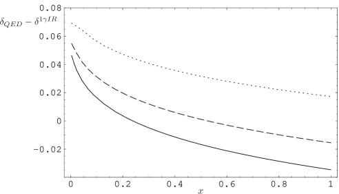
Figure 5: The traditional QED corrections (without $1\gamma IR$ contributions) for different detector resolutions $\Delta E=10\,$MeV (solid curve), 15 MeV (dashed curve) and 30 MeV (dotted curve).

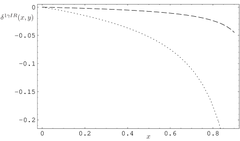
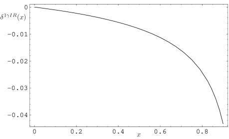
Figure 6: The one-photon irreducible corrections (triangle and box diagrams): the dashed line represents $\delta(x,0)$, the dotted line $\delta(x,y_{max})$, and the solid line on the right $\delta(x)$.

In the latter two we use the value of ${\chi}^{r}(M_{V})$ mentioned above. As we have discussed in the previous section, $\delta^{1\gamma IR}(x)$ can be safely approximated with its $m\rightarrow 0$ limit (3.24) for almost the whole range of $x$; the same is true for $\delta^{1\gamma IR}(x,y)$ for $|y|<y_{\max}(x)$, the difference between $\delta^{1\gamma IR}(x,y)$ and (3.23) can be seen for $y\sim y_{\max}(x)$ in Fig. 7.

Figure 7: The difference between $\delta^{1\gamma IR}(x,y_{max})$ (dotted line) and $\delta^{1\gamma IR}(x,y_{max})|_{m\rightarrow 0}$ (dashed line).

From these figures we can conclude, in agreement with [14], that the usually neglected $1\gamma IR$ corrections $\delta^{1\gamma IR}(x)$ are in fact important particularly in the region $x\gtrsim 0.6$, where they are in absolute value larger than $1\%$ (up to $\sim 4\%$ for $x\sim 0.9$), and comparable with $\delta_{NLO}^{1\gamma R}|_{\gamma,\psi\,loops}+\delta^{B}$; the same is true for $\delta^{1\gamma IR}(x,y)$, which is almost independent on $y$ (except for a very narrow region near $|y|\sim y_{\max}(x)$, cf. previous section). The complete pure electromagnetic corrections $\delta_{QED}(x)$ and $\delta_{QED}(x,y)$ are represented in Fig. 8.

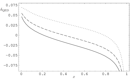
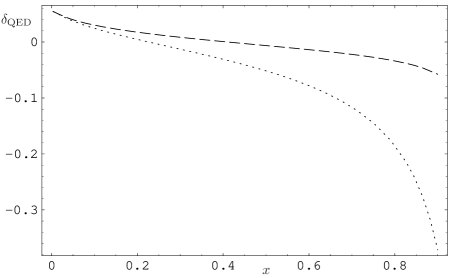
Figure 8: On the left hand side, the complete electromagnetic corrections $\delta_{QED}$ with the same detector resolutions as in Fig. 5. The right hand side shows $\delta_{QED}(x,y_{max})$ (dotted curve) and $\delta_{QED}(x,0)$ (dashed curve).

Let us now change the point of view a little bit, and split the corrections in the way we have described in the beginning of this section, namely

$$\delta_{NLO}=\delta^{\text{known}}+\delta_{NLO}^{LEC}.$$

Here $\delta^{\text{known}}$ differs from $\delta_{QED}$ (with $\overline{\chi}$ set to zero) by the contribution of $\overline{\Pi}_{\pi^{\pm}}(xM_{\pi^{0}}^{2})$ as well as by corrections stemming from chiral pion loops,

$$\delta^{\text{known}}(x,y)=\delta_{QED}(x,y)|_{\overline{\chi}=0}+2\mathrm{Re}\left[-\overline{\Pi}_{\pi^{\pm}}(xM_{\pi^{0}}^{2})+\overline{a_{NLO}^{ChPT}}(xM_{\pi^{0}}^{2})\right],$$

where

$$\overline{a_{NLO}^{ChPT}}(l^{2})=\frac{M_{\pi^{\pm}}^{2}}{16\pi^{2}F_{\pi}^{2}}\left[\ln\frac{M_{\pi^{\pm}}^{2}}{M_{\pi^{0}}^{2}}-\frac{l^{2}}{6M_{\pi^{\pm}}^{2}}\left(\frac{1}{3}+\ln\frac{M_{\pi^{\pm}}^{2}}{M_{\pi^{0}}^{2}}-16\pi^{2}\sigma_{\pi^{+}}^{2}(l^{2}){\bar{J}}_{\pi^{+}}(l^{2})\right)\right].$$ (4.4)

Separation of the numerically unambiguous part $\delta^{\text{known}}$ allows, at least in principle, to constrain the relevant combinations of the chiral low energy constants ${\cal C}_{1}^{r}$, ${\cal C}_{2}^{r}$ and ${\cal K}_{F}$ from experiment. Fig. 9 shows both $\delta^{\text{known}}$ and $\delta_{NLO}$, which allows to appreciate the effect of the counterterms.

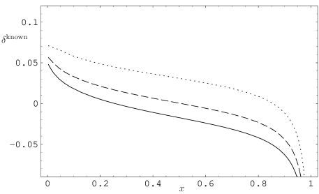
Figure 9: The NLO correction $\delta^{\text{known}}(x)$, without counterterm contributions (left), and the complete correction $\delta_{NLO}(x)$ (right). The error bars show the uncertainties coming from the counterterm determinations. The detector resolutions are as in Fig. 5.

The difference $\delta^{\text{known}}(x)-\delta_{QED}(x)$ is particularly important for $x\gtrsim 0.7$, where it represents a correction larger than $1\%$.

Let us split further

$$\delta_{NLO}^{LEC}=\delta_{LMD}^{LEC}+\delta_{QED}^{LEC},$$

where $\delta_{LMD}^{LEC}=\delta_{NLO}^{LEC}|_{{{\cal K}_{F}}=0}$ is the part for which we have theoretical prediction based on the LMD approximation; $\delta^{\text{known}}+\delta_{LMD}^{LEC}$ is shown in the Fig. 9, the error band stems from the estimate of the uncertainty of the LMD values (4.1).

For completeness, we present our theoretical estimate of $\delta_{QED}^{LEC}$, based on (C.26) (cf. (4.1)),

$$\delta_{QED}^{LEC}(x,y)=\delta_{QED}^{LEC}(x)=\frac{e^{2}}{32\pi^{2}}{\cal K}_{F}=(-8\pm 2)\times 10^{-3}.$$

Note that this value is comparable with the estimated uncertainty of $\delta_{LMD}^{LEC}$ arising from the uncertainties in ${\cal C}_{1}$ and ${\cal C}_{2}^{r}(\mu=M_{V})$ as given in Eq. (4.1).

4.3 Decay rate

Let us make a brief comment on the total decay rate. At the leading order we reproduce the old Dalitz result [2]:

$$\frac{\Gamma^{\text{LO}}(\pi^{0}\rightarrow e^{+}e^{-}\gamma)}{\Gamma(\pi^{0}\rightarrow 2\gamma)}=\frac{\alpha}{\pi}\Bigl{(}\frac{4}{3}\ln\frac{M_{\pi^{0}}}{m}-\frac{7}{3}+O(\nu^{2})\Bigr{)}=0.01185,$$

which should be compared with the present experimental value [1]:

$$\frac{\Gamma^{\text{exp}}(\pi^{0}\rightarrow e^{+}e^{-}\gamma)}{\Gamma(\pi^{0}\rightarrow 2\gamma)}=0.01213\pm 0.00033.$$ (4.5)

As already mentioned in the Introduction, the traditional radiative corrections to the total decay rate are tiny. The corrections corresponding to the first and second term in the decomposition of the QED corrections (4.2) were first numerically evaluated in [11] and analytically in [12] with the result:

$$\frac{\Gamma^{\text{NLO}}_{\text{QED}}(\pi^{0}\rightarrow e^{+}e^{-}\gamma)}{\Gamma(\pi^{0}\rightarrow 2\gamma)} =\Bigl{(}\frac{\alpha}{\pi}\Bigr{)}^{2}\Bigl{(}\frac{8}{9}\ln^{2}{\frac{M_{\pi^{0}}}{m}}-\frac{19}{9}\ln{\frac{M_{\pi^{0}}}{m}}+2\zeta(3)+\frac{137}{81}-\frac{2}{27}\pi^{2}+O(\nu)\Bigr{)}$$

$$=1.04\times 10^{-4}.$$ (4.6)

Let us note that this formula is not based on the soft photon approximation, but the whole energy spectrum of the bremsstrahlung photon is included. A real photon emitted from the pion vertex is not considered. If we take into account the remaining NLO $1\gamma R$ (ChPT corrections) and $1\gamma IR$ electromagnetic corrections we get an additional contribution

$$\frac{\Gamma^{\text{NLO}}_{\text{ChPT}+1\gamma IR}(\pi^{0}\rightarrow e^{+}e^{-}\gamma)}{\Gamma(\pi^{0}\rightarrow 2\gamma)}=(1.8\pm 0.6)\times 10^{-5},$$ (4.7)

where the error stems from uncertainty of ${\cal C}_{2}$. Clearly these two corrections are small in comparison with the present experimental uncertainty (4.5).

Similarly we could evaluate the corrected rate in the soft-photon approximation. The result then depends on $\Delta E$. For $\Delta E\sim 10MeV$, for instance, the result reads $\frac{\Gamma^{\text{NLO}}}{\Gamma_{2\gamma}}\simeq 4\times 10^{-4}$.

4.4 Slope parameter

We have now all the elements at hand in order to discuss both the extraction of the slope parameter from the data, and the prediction that can be made for it in the framework of the low energy theory. With the help of the formulae (3.10), (C.23), (D.2) and the definition (3.6) we easily find

$$a_{\pi}=\frac{M_{\pi^{0}}^{2}}{M_{\pi^{\pm}}^{2}}\left[\frac{1}{6}\,{\cal C}_{2}-\frac{M_{\pi^{\pm}}^{2}}{96\pi^{2}F_{\pi}^{2}}\left(1+\ln\left(\frac{M_{\pi^{\pm}}^{2}}{M_{V}^{2}}\right)\right)-\frac{1}{360}\left(\frac{\alpha}{\pi}\right)\right],$$ (4.8)

where the individual terms in the square bracket correspond to the counterterm, the charged pion chiral loops, and the charged pion vacuum polarization function contribution, respectively (the latter we include here only for the sake of completeness, numerically it is negligible, being of the order $10^{-6}$, and thus can be safely neglected). Using the previous inputs, we obtain the following theoretical prediction for the slope parameter

$$a_{\pi}\,=\,0.029\pm 0.005.$$ (4.9)

As we have noted in the preceding section, previous experimental analyses, as a rule, did not include the contribution of the two-photon exchange (which was treated as negligible due to the superficial arguments based on the Low theorem). Therefore, according to the formula (3.6), the systematic bias due to this omission can be roughly estimated as, cf. (3.24),

$$\Delta a_{\pi}\bigg{|}_{1\gamma IR}=-\frac{1}{2}\frac{d\delta^{1\gamma IR}(x)|_{m\rightarrow 0}}{dx}\bigg{|}_{x=0}=\frac{1}{8}\left(\frac{\alpha}{\pi}\right)(2\pi^{2}-3)\doteq 0.005.$$ (4.10)

This corresponds to a shift of the central values for $a_{\pi}$ extracted from the Dalitz decay measurements which goes into the right direction towards the independent CELLO result.

5 Summary and conclusions

The present work provides a detailed analysis of next-to-leading order radiative corrections to the Dalitz decay amplitude. This study involves the off-shell pion-photon transition form factor, which requires a treatment of non perturbative strong interaction effects. We have relied on representations of this form factor involving zero-width vector resonances. In contrast to the simplest vector meson dominance representation, our approach satisfies various short distance constraints from QCD. Our analysis also includes the one-photon irreducible contributions, which were usually neglected. We have shown that, although these contributions are negligible as far as the corrections to the total decay rate are concerned, they are however sizeable in regions of the Dalitz plot which are relevant for the determination of the slope parameter $a_{\pi}$ of the pion-photon transition form factor. We have also obtained a prediction for $a_{\pi}$ which is in good agreement with the determinations obtained from the (model dependent) extrapolation of the CELLO and CLEO data. The present difference with the central values directly measured in the latest Dalitz decay experiments can be ascribed to the omission of the radiative corrections induced by the one-photon irreducible contributions. Unfortunately, the experimental error bars on the latest values of $a_{\pi}$ extracted from the Dalitz decay are still too large to make a comparison with the CELLO and CLEO values meaningful. Nevertheless, we think that a precise measurement of $a_{\pi}$ which would not rely on any kind of extrapolation remains an interesting issue. Hopefully, future experiments, like the one proposed by the PrimEx collaboration at TJNAF, will improve the situation in this respect.

Acknowledgements. We wish to thank J. Hořejší for comments on the manuscript, as well as J. Schacher, L. Nemenov, and A. Bernstein for interesting discussions and/or correspondences. We are also grateful to B. Moussallam for a useful discussion concerning the $SU(3)$ matching. K. K. and J. N. are supported in part by the program Research Centres , project number LC05A02A of the Ministry of Education of the Czech Republic. The work of M. K. is supported in part by the EC contract No. HPRN-CT-2002-00311 (EURIDICE). This work was initiated during a stay of K. K. at Centre de Physique Théorique, partially financed by the SOCRATES/ERASMUS student exchange program.

Appendix A Form factor projectors

Here we list the projectors $\Lambda_{F}^{\mu}$ which allow to obtain the form factors $F=P$, $A_{\pm}$ and $T$ from Eq. (2.7). One possible choice is

$$\Lambda_{P}^{\mu} = \frac{1}{2\Delta^{2}\delta^{2}}\mathrm{i}\varepsilon^{\mu\nu\alpha\beta}k_{\nu}p_{+\alpha}p_{-\beta}-\frac{m}{4\Delta^{4}}(k\cdot q)(k\cdot\delta)[\gamma^{\mu}(k\cdot q)-q^{\mu}\not{k}]\gamma_{5}$$ (A.1)

$$+\frac{m}{4\Delta^{4}\delta^{2}}[2\Delta^{2}-q^{2}(k\cdot\delta)^{2}][\gamma^{\mu}k\cdot\delta-\delta^{\mu}\not{k}]\gamma_{5}$$

$$-\frac{1}{4\Delta^{2}\delta^{4}}[2\Delta^{2}-((k\cdot q)^{2}-(k\cdot\delta)^{2})\delta^{2}]\Delta^{\mu}\gamma_{5},$$

$$\Lambda_{A_{\pm}}^{\mu} = \frac{m}{2\Delta^{2}\delta^{2}}\mathrm{i}\varepsilon^{\mu\nu\alpha\beta}k_{\nu}p_{+\alpha}p_{-\beta}\mp\frac{1}{16\Delta^{4}}[2\Delta^{2}+q^{2}(k\cdot(q\mp\delta))(k\cdot\delta)][\gamma^{\mu}(k\cdot q)-q^{\mu}\not{k}]\gamma_{5}$$ (A.2)

$$-\frac{q^{2}}{32\Delta^{4}\delta^{2}}[4\Delta^{2}-2(k\cdot(q\mp\delta))(k\cdot q)\delta^{2}+m^{2\,}(k\cdot(q\mp\delta))^{2}][\gamma^{\mu}k\cdot\delta-\delta^{\mu}\not{k}]\gamma_{5}$$

$$-\frac{m}{8\Delta^{4}\delta^{2}}[4\Delta^{2}-2(k\cdot(q\mp\delta))(k\cdot q)\delta^{2}+m^{2\,}(k\cdot(q\mp\delta))^{2}]\Delta^{\mu}\gamma_{5},$$

$$\Lambda_{T}^{\mu} = \frac{1}{4\Delta^{2}}\mathrm{i}\varepsilon^{\mu\nu\alpha\beta}k_{\nu}p_{+\alpha}p_{-\beta},$$ (A.3)

where we have introduced the shorthand notation $q=p_{+}+p_{-}$, $\Delta=(k\cdot p_{+})p_{-}-(k\cdot p_{-})p_{+}$, and $\delta=p_{+}-p_{-}$. In the limit $m\rightarrow 0$ these expressions simplify to the form

$$\Lambda_{P}^{\mu} = \frac{1}{2\Delta^{2}\delta^{2}}\mathrm{i}\varepsilon^{\mu\nu\alpha\beta}k_{\nu}p_{+\alpha}p_{-\beta}-\frac{1}{2\Delta^{2}\delta^{4}}[\Delta^{2}-2(k\cdot p_{+})(k\cdot p_{-})\delta^{2}]\Delta^{\mu}\gamma_{5},$$ (A.4)

$$\Lambda_{A_{\pm}}^{\mu} = \mp\frac{1}{16\Delta^{4}}[2\Delta^{2}+q^{2}(k\cdot(q\mp\delta))(k\cdot\delta)][\gamma^{\mu}(k\cdot q)-q^{\mu}\not{k}]\gamma_{5}$$ (A.5)

$$-\frac{q^{2}}{32\Delta^{4}\delta^{2}}[4\Delta^{2}-2(k\cdot(q\mp\delta))(k\cdot q)\delta^{2}][\gamma^{\mu}k\cdot\delta-\delta^{\mu}\not{k}]\gamma_{5},$$

$$\Lambda_{T}^{\mu} = \frac{1}{4\Delta^{2}}\mathrm{i}\varepsilon^{\mu\nu\alpha\beta}k_{\nu}p_{+\alpha}p_{-\beta}.$$ (A.6)

Appendix B The pion-photon-photon vertex

As we have seen in the main text, the doubly off-shell $\pi^{0}$-$\gamma^{*}$-$\gamma^{*}$ vertex, defined as

$$\int d^{4}x\,e^{il\cdot x}\langle 0|T\{j^{\mu}(x)j^{\nu}(0)\}|\pi^{0}(P)\rangle=-\mathrm{i}\varepsilon^{\mu\nu\alpha\beta}l_{\alpha}p_{\beta}\mathcal{A}_{\pi^{0}\gamma^{*}\gamma^{*}}(l^{2},(P-l)^{2}),$$

is a necessary ingredient for the calculation of the Dalitz decay amplitude. While in the case of the one-photon reducible contribution it is sufficient to use the corresponding form factor $\mathcal{A}_{\pi^{0}\gamma^{*}\gamma^{*}}(0,l^{2})$ for $l^{2}\lesssim M_{\pi}^{2}$, which is the region where ChPT (with virtual photons) is applicable, for the leading one-fermion reducible and one-particle irreducible contributions it is necessary to know $\mathcal{A}_{\pi^{0}\gamma^{*}\gamma^{*}}(l^{2},(P-l)^{2})$ as a function of the momentum $l$ in the full range of the loop integration. In the present Appendix, we neglect temporarily the electromagnetic interaction, so that $\mathcal{A}_{\pi^{0}\gamma^{*}\gamma^{*}}(l^{2},(P-l)^{2})$ will refer to the strong matrix element. We briefly summarize some basic properties of the form factor $\mathcal{A}_{\pi^{0}\gamma^{*}\gamma^{*}}(l^{2},(P-l)^{2})$ that are general consequences of QCD, as well as the results of [27], which we shall use in the sequel. The low energy expansion of $\mathcal{A}_{\pi^{0}\gamma^{*}\gamma^{*}}$ in the presence of both strong and electromagnetic interactions will be the subject of the next Appendix.

General properties of the form factor $\mathcal{A}_{\pi^{0}\gamma^{*}\gamma^{*}}(l^{2},(P-l)^{2})$ in QCD were investigated earlier within various approaches [40, 41]. In the chiral limit, the on-shell value of the form factor is entirely fixed by the QCD chiral anomaly. Therefore, within ChPT the low energy behaviour is expected to be

$$\mathcal{A}_{\pi^{0}\gamma^{*}\gamma^{*}}(l^{2},(P-l)^{2})=-\frac{N_{C}}{12\pi^{2}F_{\pi}}\left[1+{\cal O}\left(\frac{P\cdot l}{\Lambda_{H}^{2}},\frac{l^{2}}{\Lambda_{H}^{2}},\frac{m_{q}}{\Lambda_{H}}\right)\right],$$ (B.1)

where the higher order corrections come from pseudo-Goldstone boson loops, as well as from higher order contact terms. In particular,

$$\mathcal{A}_{\pi^{0}\gamma^{*}\gamma^{*}}(0,0)=-\frac{N_{C}}{12\pi^{2}F_{\pi}}\left[1+{\cal O}\left(\frac{m_{q}}{\Lambda_{H}}\right)\right].$$ (B.2)

Another exact result, the leading short distance asymptotics for $l\rightarrow\infty$, ($P$ fixed), follows from the operator product expansion (see [43]). For $\lambda\rightarrow\infty$ we have

$$\mathcal{A}_{\pi^{0}\gamma^{*}\gamma^{*}}((\lambda l)^{2},(P-\lambda l)^{2})=\frac{1}{(\lambda l)^{2}}\frac{2}{3}F_{\pi}\left[1\,+\,\frac{1}{\lambda}\,\frac{P\cdot l}{l^{2}}\,+\,\cdots\right].$$ (B.3)

The ellipsis stands for higher order terms in the short-distance expansion, or for ${\cal O}(\alpha_{s})$ QCD corrections to the terms that are shown. Notice that the latter are not affected by quark mass effects, so that Eq. (B.3) holds beyond the chiral limit. On the other hand, the expression (B.3) assumes isospin and CP invariance of the strong interactions. The explicit form of $\mathcal{A}_{\pi^{0}\gamma^{*}\gamma^{*}}(l^{2},(P-l)^{2})$ in the intermediate energy range, however, is not known from first principles. Among the various approaches that have been considered, models inspired by the large-$N_{C}$ properties of QCD have been proven particularly useful in order to provide parameterizations of the form factor $\mathcal{A}_{\pi^{0}\gamma^{*}\gamma^{*}}(l^{2},(P-l)^{2})$ compatible with the above low and high energy behaviours predicted by QCD. Let us give here a brief overview of the results obtained in Ref. [27] within this framework. At leading order in the $1/N_{C}$ expansion, $\mathcal{A}_{\pi^{0}\gamma^{*}\gamma^{*}}(l^{2},(P-l)^{2})$ can be expressed as infinite sum of the tree-level exchanges of the zero-width resonances in the various channels. Truncating this infinite sum and keeping only the contribution of the lowest resonances, i.e. the lowest vector meson octet in the present case, we obtain the Lowest Meson Dominance approximation (LMD) to the large-$N_{C}$ expression [26]

$$\mathcal{A}_{\pi^{0}\gamma^{*}\gamma^{*}}^{LMD}(l^{2},(P-l)^{2})=\frac{F_{\pi}}{3}\frac{l^{2}+(P-l)^{2}+\kappa_{V}}{(l^{2}-M_{V}^{2})((P-l)^{2}-M_{V}^{2})}.$$ (B.4)

This Ansatz satisfies all the properties of $\mathcal{A}_{\pi^{0}\gamma^{*}\gamma^{*}}$ discussed so far, provided the constant $\kappa_{V}$ is chosen such as to provide compatibility with (B.1),

$$\kappa_{V}=\frac{3M_{V}^{4}}{F_{\pi}}\,\mathcal{A}_{\pi^{0}\gamma^{*}\gamma^{*}}(0,0)=-\,\frac{N_{C}}{4\pi^{2}F_{\pi}^{2}}M_{V}^{4}(1+{\cal C}_{1}+\cdots).$$ (B.5)

The second equality involves the leading quark mass corrections described by the combination of low energy constants given in Eqs. (C.15) and (C.16) below, while the ellipsis stands for higher order quark mass corrections, that will not be considered here. Let us note that if the large-$N_{C}$ vector meson mass is identified with the physical mass of the $\rho$ meson, $M_{V}=M_{\rho}$, the form factor $\mathcal{A}_{\pi^{0}\gamma^{*}\gamma^{*}}^{LMD}(l^{2},(P-l)^{2})$ contains ${\cal C}_{1}$ as the only free parameter, and interpolates smoothly between (B.1) and (B.3). On the other hand, at low energy, the non-analytical contributions from Goldstone boson intermediate states are not taken into account (note that according to the large-$N_{C}$ counting rules, meson loops are suppressed in the $1/N_{C}$ expansion). As further discussed in [27], the simple Ansatz (B.4) is not sufficient to describe the full asymptotic behaviour for $Q^{2}\rightarrow\infty$, where $Q^{2}=-(q_{1}^{2}+q_{2}^{2})$ with fixed $\omega=(q_{1}^{2}-q_{2}^{2})/(q_{1}^{2}+q_{2}^{2})=\pm 1$, given by the general formula [41]

$$\mathcal{A}_{\pi^{0}\gamma^{*}\gamma^{*}}(q_{1}^{2},q_{2}^{2})=-\,\frac{4F_{\pi}}{3}\,\frac{f(\omega)}{Q^{2}}+\mathcal{O}\left(\frac{1}{Q^{4}}\right)\,,$$ (B.6)

with a function $f(\omega)$ that is not known explicitly. In order to reconcile the large $N_{C}$ ansatz with (B.6), at least one additional vector resonance is unavoidable. We thus obtain, in the notation of [27], the more general Ansatz

$$\mathcal{A}_{\pi^{0}\gamma^{*}\gamma^{*}}^{LMD+V}(q_{1}^{2},q_{2}^{2})=\frac{F_{\pi}}{3}\frac{q_{1}^{2}q_{2}^{2}(q_{1}^{2}+q_{2}^{2})+\kappa_{1}(q_{1}^{2}+q_{2}^{2})^{2}+\kappa_{2}q_{1}^{2}q_{2}^{2}+\kappa_{5}(q_{1}^{2}+q_{2}^{2})+\kappa_{7}}{(q_{1}^{2}-M_{V_{1}}^{2})(q_{1}^{2}-M_{V_{2}}^{2})(q_{2}^{2}-M_{V_{1}}^{2})(q_{2}^{2}-M_{V_{2}}^{2})}\,.$$ (B.7)

The chiral anomaly fixes now

$$\kappa_{7}=\frac{3M_{V_{1}}^{4}M_{V_{2}}^{4}}{F_{\pi}}\,\mathcal{A}_{\pi^{0}\gamma^{*}\gamma^{*}}(0,0)=-\,\frac{N_{C}}{4\pi^{2}}\frac{M_{V_{1}}^{4}M_{V_{2}}^{4}}{F_{\pi}^{2}}(1+{\cal C}_{1}+\cdots),$$ (B.8)

while the large $Q^{2}$ behaviour of $\mathcal{A}_{\pi^{0}\gamma^{*}\gamma^{*}}(Q^{2},0)$ requires $\kappa_{1}=0$. From experimental data one can also determine

$$\kappa_{5}=6.93\pm 0.26\,\mathrm{GeV}^{4},$$ (B.9)

(one takes $M_{V_{1}}=769\,\mathrm{MeV}$, $M_{V_{2}}=1465\,\mathrm{MeV}$, $F_{\pi}=92.4\,\mathrm{MeV,}$ further details can be found in [27]). Finally, as pointed out in Ref. [42], the coefficient $\kappa_{2}$ is also available from Ref. [43],

$$\kappa_{2}\sim-4(M_{V_{1}}^{2}+M_{V_{2}}^{2})=-10\,\mathrm{GeV}^{2},$$ (B.10)

a value which lies within the range considered in Ref. [27].

Appendix C Chiral Expansion of the pion-photon-photon vertex

In this Appendix, we first summarize the results of our recalculation of the pure QCD form factor $\mathcal{A}_{\pi^{0}\gamma^{*}\gamma^{*}}(0,l^{2})$ in two-flavour Chiral Perturbation Theory [17, 20, 44, 30] up to one loop, i.e. up to the order $\mathcal{O}(p^{6})$. After that, we describe the additional modifications that appear if electromagnetic effects are also included.

C.1 $e=0$

The relevant chiral Lagrangian can be written in the form

$$\mathcal{L=L}^{(2)}+\mathcal{L}^{(4)}+\mathcal{L}_{WZW}^{(4)}+\mathcal{L}^{(6)}+\ldots,$$

where the terms with even intrinsic parity at order $O(p^{2})$ and $O(p^{4})$ are

$$\mathcal{L}^{(2)} = \frac{F_{0}^{2}}{4}\langle D^{\mu}U^{+}D_{\mu}U+\chi^{+}U+U^{+}\chi\rangle$$ (C.1)

$$\mathcal{L}^{(4)} = \frac{l_{1}}{4}\langle D^{\mu}U^{+}D_{\mu}U\rangle^{2}+\frac{l_{2}}{4}\langle D^{\mu}U^{+}D^{\nu}U\rangle\langle D_{\mu}U^{+}D_{\nu}U\rangle$$ (C.2)

$$+\frac{l_{3}}{16}\langle\chi^{+}U+U^{+}\chi\rangle^{2}+\frac{l_{4}}{4}\langle D_{\mu}UD^{\mu}\chi^{+}+D^{\mu}U^{+}D_{\mu}\chi\rangle$$

$$+l_{5}\langle\widehat{R}_{\mu\nu}U\widehat{L}^{\mu\nu}U^{+}\rangle+\mathrm{i}\frac{l_{6}}{2}(\langle\widehat{R}_{\mu\nu}D^{\mu}UD^{\nu}U^{+}\rangle+\langle\widehat{L}_{\mu\nu}D^{\mu}U^{+}D^{\nu}U\rangle)$$

$$-\frac{l_{7}}{16}\langle\chi^{+}U-U^{+}\chi\rangle^{2}$$

$$+\frac{1}{4}(h_{1}+h_{3})\langle\chi^{+}\chi\rangle+\frac{1}{4}(h_{1}-h_{3})(\det\chi^{+}+\det\chi)$$

$$-\frac{1}{2}(l_{5}+4h_{2})\langle\widehat{R}_{\mu\nu}\widehat{R}^{\mu\nu}+\widehat{L}_{\mu\nu}\widehat{L}^{\mu\nu}\rangle+\frac{h_{4}}{4}\langle R_{\mu\nu}+L_{\mu\nu}\rangle\langle R^{\mu\nu}+L^{\mu\nu}\rangle$$

$$+\frac{h_{5}}{4}\langle R_{\mu\nu}-L_{\mu\nu}\rangle\langle R^{\mu\nu}-L^{\mu\nu}\rangle).$$

The odd intrinsic parity Wess-Zumino-Witten Lagrangian, which accounts for the two-flavour anomaly can be written in the form [44]

$$\mathcal{L}_{WZW}^{(4)} = -\frac{N_{C}}{32\pi^{2}}\varepsilon^{\mu\nu\rho\sigma}[\langle U^{+}\widehat{r}_{\mu}U\widehat{l}_{\nu}-\widehat{r}_{\mu}\widehat{l}_{\nu}+\mathrm{i}\Sigma_{\mu}(U^{+}\widehat{r}_{\nu}U+\widehat{l}_{\nu})\rangle\langle v_{\rho\sigma}\rangle$$ (C.3)

$$+\frac{2}{3}\langle\Sigma_{\mu}\Sigma_{\nu}\Sigma_{\rho}\rangle\langle v_{\sigma}\rangle].$$

In the above formulae, the notation is as follows:

$$U = \mathrm{e}^{\frac{\mathrm{i}\phi}{F_{0}}},\quad\phi=\left(\begin{array}[]{cc}\pi^{0}&\sqrt{2}\pi^{+}\\ \sqrt{2}\pi^{-}&-\pi^{0}\end{array}\right),$$ (C.6)

$$D_{\mu}U = \partial_{\mu}U-\mathrm{i}r_{\mu}U+\mathrm{i}Ul_{\mu},\,\,\,\,\Sigma_{\mu}=U^{+}\partial_{\mu}U,$$ (C.7)

$$R_{\mu\nu} = \partial_{\mu}r_{\nu}-\partial_{\nu}r_{\mu}-\mathrm{i}[r_{\mu},r_{\nu}],\,\,\,L_{\mu\nu}=\partial_{\mu}l_{\nu}-\partial_{\nu}l_{\mu}-\mathrm{i}[l_{\mu},l_{\nu}],$$ (C.8)

$$\widehat{R}_{\mu\nu} = R_{\mu\nu}-\frac{1}{2}\langle R_{\mu\nu}\rangle,\,\,\,\,\widehat{L}_{\mu\nu}=L_{\mu\nu}-\frac{1}{2}\langle L_{\mu\nu}\rangle,$$ (C.9)

$$\widehat{r}_{\mu} = r_{\mu}-\frac{1}{2}\langle r_{\mu}\rangle,\,\,\,\widehat{l}_{\mu}=l_{\mu}-\frac{1}{2}\langle l_{\mu}\rangle,$$ (C.10)

$$v_{\mu} = \frac{1}{2}(r_{\mu}+l_{\mu}),\,\,\,v_{\mu\nu}=\partial_{\mu}v_{\nu}-\partial_{\nu}v_{\mu}-\mathrm{i}[v_{\mu},v_{\nu}].$$ (C.11)

Further relevant chiral invariant Lagrangians of order $\mathcal{O}(p^{6})$ and also the other details can be found in [45, 46] and references therein.

The form factor $\mathcal{A}_{\pi^{0}\gamma^{*}\gamma^{*}}(0,l^{2})$ starts at the order $\mathcal{O}(p^{4})$ with the tree graph with vertex derived from the Wess-Zumino-Witten Lagrangian (C.3), and reproduces the anomaly result (B.1),

$$\mathcal{A}_{\pi^{0}\gamma^{*}\gamma^{*}}^{LO}(0,l^{2})=-\,\frac{N_{C}}{12\pi^{2}F_{0}},$$ (C.12)

since $F_{0}$ can be identified with $F_{\pi}$ at this order. At the next-to-leading order, there are two types of one-loop contributions with one vertex from $\mathcal{L}_{WZW}^{(4)}$, namely the tadpole and the bubble graphs (see Fig. 10).

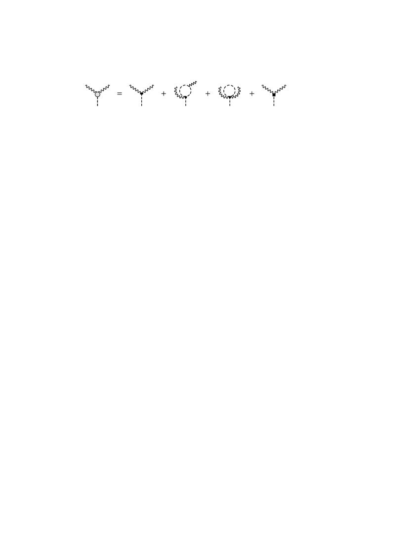
Figure 10: Next-to-leading order corrections to $\pi\gamma\gamma$ vertex.

Another type of contributions correspond to the contact terms derived from the tree graphs with one vertex from the odd intrinsic parity part of $\mathcal{L}^{(6)}$. A last contribution comes from the renormalization factor of the external pion leg; this one contains the tadpole with vertex from $\mathcal{L}^{(2)}$ and contact terms with vertices from $\mathcal{L}^{(4)}$, see Fig. 11.

Figure 11: $\pi^{0}$ wave function renormalization in next-to-leading order.

Putting all these parts together we obtain the following result

$$\mathcal{A}_{\pi^{0}\gamma^{*}\gamma^{*}}(0,l^{2})=-\frac{N_{C}}{12\pi^{2}F_{\pi}}\Bigl{\{}1+{\cal C}_{1}-\frac{l^{2}}{6M_{\pi}^{2}}\Bigl{[}\left(\frac{M_{\pi}}{4\pi F_{\pi}}\right)^{2}\left(\tfrac{1}{3}-16\pi^{2}\sigma_{\pi}^{2}(l^{2}){\bar{J}}_{\pi}(l^{2})\right)-{\cal C}_{2}\Bigr{]}\Bigr{\}},$$ (C.13)

where $\sigma_{P}(s)\equiv\sqrt{1-4M_{P}^{2}/s}$ and

$${\bar{J}}_{P}(s)=\frac{s}{16\pi^{2}}\int_{4M_{P}^{2}}^{\infty}\frac{\mathrm{d}x}{x}\frac{\sigma_{P}(x)}{x-s}$$ (C.14)

is the Chew-Mandelstam function (the scalar bubble subtracted at $s=0$). In the above formula, we keep the neutral and charged pion masses equal (within pure QCD their difference is an effect of second order in the isospin breaking parameter $(m_{u}-m_{d})$), the isospin breaking QED corrections, which are, taking $e=O(p)$, of the same order as the leading order terms, will be taken into account in the next section where further details can be found. Finally, ${\cal C}_{1}$ and ${\cal C}_{2}$ represent the following renormalization-scale independent combinations of the $O(p^{6})$ low energy constants $A_{i}$ and $c_{i}$ introduced in [45] and [46] respectively:

$${\cal C}_{1} = \frac{32}{3}\pi^{2}\Bigl{[}(A_{2}^{r}-2A_{3}^{r}-4A_{4}^{r})M_{\pi}^{2}+\frac{20}{3}(A_{4}^{r}+2A_{6}^{r})2\bar{m}B\Bigr{]}$$

$$= \frac{64}{3}\pi^{2}\Bigl{[}(c_{11}^{r}-4c_{3}^{r}-4c_{7}^{r})M_{\pi}^{2}+\frac{4}{3}(5c_{3}^{r}+c_{7}^{r}+2c_{8}^{r})2\bar{m}B\Bigr{]},$$

$${\cal C}_{2} = {\cal C}_{2}^{r}(\mu)-\left(\frac{M_{\pi}}{4\pi F_{\pi}}\right)^{2}\ln\frac{M_{\pi}^{2}}{\mu^{2}},$$ (C.15)

with $\bar{m}=(m_{d}-m_{u})/2$ and

$${\cal C}_{2}^{r}(\mu)\,=\,-64\pi^{2}M_{\pi}^{2}(A_{2}^{r}-4A_{3}^{r})=-64\pi^{2}M_{\pi}^{2}c_{13}^{r}.$$ (C.16)

The renormalization of the external pion line is responsible for the replacement of the constant $F_{0}$ with the physical decay constant $F_{\pi}$ in the leading order term of (C.13).

The actual values of the constants ${\cal C}_{1}$ and ${\cal C}_{2}$ are not known from first principles. Recently the relevant combinations of the low energy constants that occur in ${\cal C}_{2}$ have been estimated in [27] by using the matching of the LMD approximation to the large $N_{C}$ form factor $\mathcal{A}_{LMD}(l^{2},0)$ and the large $N_{C}$ approximation to the ChPT result $\mathcal{A}^{ChPT}(l^{2},0)$. Since in the large-$N_{C}$ limit the contribution of meson loops is suppressed, the chiral logarithms as well as the running of the renormalized couplings with the renormalization scale $\mu$ are next-to-leading order effects. Following [47], we assume that the values of the low energy constants obtained this way correspond to scale given by the mass scale of the non-Goldstone resonances $\mu\sim M_{V}$. We thus have the following LMD determination of the low energy constant ${\cal C}_{2}$ [27]:

$${\cal C}_{2}^{r}(M_{V})_{LMD}=6\Bigl{[}1+{\cal C}_{1}-\frac{1}{4N_{C}}\Bigl{(}\frac{4\pi F_{\pi}}{M_{V}}\Bigr{)}^{2}\Bigr{]}\Bigl{(}\frac{M_{\pi}}{M_{V}}\Bigr{)}^{2}.$$ (C.17)

The same procedure can be done with the $LMD+V$ approximation; in this case we find [27]

$${\cal C}_{2}^{r}(M_{V})_{LMD+V}=6\Bigl{(}\frac{M_{\pi}}{4\pi F_{\pi}}\Bigr{)}^{2}\Bigl{[}(1+{\cal C}_{1})\Bigl{(}\Bigl{(}\frac{4\pi F_{\pi}}{M_{V_{1}}}\Bigr{)}^{2}+\Bigl{(}\frac{4\pi F_{\pi}}{M_{V_{2}}}\Bigr{)}^{2}\Bigr{)}\\ -\frac{1}{4N_{C}}\Bigl{(}\frac{4\pi F_{\pi}}{M_{V_{1}}}\Bigr{)}^{2}\Bigl{(}\frac{4\pi F_{\pi}}{M_{V_{2}}}\Bigr{)}^{2}\frac{\kappa_{5}}{M_{V_{1}}^{2}M_{V_{2}}^{2}}\Bigr{]}.$$ (C.18)

The issue of the quark mass corrections to $\mathcal{A}_{\pi^{0}\gamma^{*}\gamma^{*}}(0,l^{2})$, contained in ${\cal C}_{1}$, have been addressed in [48], and more recently in [39]. From [39], one infers

$${\cal C}_{1}=\frac{m_{d}-m_{u}}{m_{s}-{\widehat{m}}}\,(0.93\pm 0.12)\pm 0.14\cdot 10^{-2},$$ (C.19)

with ${\widehat{m}}=(m_{u}+m_{d})/2$.

Numerically, with $(m_{d}-m_{u})/(m_{s}-{\widehat{m}})=1/43$, $M_{\pi}=135\,\mathrm{MeV}$, $F_{\pi}=92.4\,\mathrm{MeV}$, $M_{V}=M_{V_{1}}=770\,\mathrm{MeV}$, $M_{V_{2}}=1465\,\mathrm{MeV}$ and $\kappa_{5}$ given by (B.9), we then have the following determinations

$${\cal C}_{1} = (2.2\pm 0.3)\times 10^{-2},$$

$${\cal C}_{2}^{r}(M_{V})_{LMD} = (1.5\pm 0.5)\times 10^{-1},$$

$${\cal C}_{2}^{r}(M_{V})_{LMD+V} = (1.8\pm 0.6)\times 10^{-1}.$$

A 30% uncertainty, typical for a result based on a leading order large-$N_{C}$ calculation, has been assigned to ${\cal C}_{2}$. Within these error bars, the $LMD$ result is stable with respect to the inclusion of a second resonance. Notice also that a variation of the scale between, say, $M_{V}=M_{V_{1}}$ and $M_{V}=M_{V_{2}}$ gives ${\cal C}_{2}^{r}(M_{V_{1}})-{\cal C}_{2}^{r}(M_{V_{2}})=0.02$, which is well within these error bars.

C.2 $e\neq 0$

In this section we shall describe the results of our calculation of the next-to-leading $O(p^{6})$ corrections to the leading order amplitude in the expansion scheme in which the electric charge, fermion masses, and fermion bilinears are assumed to be counted as quantities of order $p$. Within this scheme, the $O(p^{2})$ Lagrangian reads

$$\mathcal{L}^{(2)} = \frac{F_{0}^{2}}{4}\langle D^{\mu}U^{+}D_{\mu}U+\chi^{+}U+U^{+}\chi\rangle+e^{2}ZF_{0}^{4}\langle QUQU^{+}\rangle$$

$$-\frac{1}{4}F_{\mu\nu}F^{\mu\nu}+\overline{\psi}(\mathrm{i}\gamma\cdot(\partial-\mathrm{i}eA)-m_{e})\psi,$$

where

$$Q=\mathrm{diag}(2/3,-1/3)$$

is the quark charge matrix. Then the leading order amplitude, which corresponds to the tree graph with one vertex from $\mathcal{L}_{WZW}^{(4)}$, is of the order $O(p^{4})$. Let us also note that electromagnetic splitting of the charged and neutral pion masses is treated as a leading order effect. The $O(p^{4})$ Lagrangian with even intrinsic parity then reads

$$\mathcal{L}^{(4)}=\mathcal{L}_{p^{4}}^{(4)}+\mathcal{L}_{e^{2}p^{2}}^{(4)}+\mathcal{L}_{lept}^{(4)}.$$

The $\mathcal{L}_{p^{4}}^{(4)}$ is the same as (C.2) while the explicit form of $\mathcal{L}_{e^{2}p^{2}}^{(4)}$ and $\mathcal{L}_{lept}^{(4)}$ can be found in [20] and [23]. In the following we need only

$$\mathcal{L}_{e^{2}p^{2}}^{(4)} = F_{0}^{2}\left\{k_{1}\langle D^{\mu}U^{+}D_{\mu}U\rangle\langle Q^{2}\rangle+k_{2}\langle D^{\mu}U^{+}D_{\mu}U\rangle\langle QUQU^{+}\rangle\right.$$

$$+k_{3}\left(\langle D^{\mu}U^{+}QU\rangle\langle D_{\mu}U^{+}QU\rangle+\langle D^{\mu}UQU^{+}\rangle\langle D_{\mu}UQU^{+}\rangle\right)$$

$$\left.+k_{4}\langle D^{\mu}U^{+}QU\rangle\langle D_{\mu}UQU^{+}\rangle+\ldots\right\},$$

$$\mathcal{L}_{lept}^{(4)} = e^{2}x_{6}\overline{\psi}(\mathrm{i}\gamma\cdot(\partial-\mathrm{i}eA))\psi+e^{2}x_{7}m_{e}\overline{\psi}\psi+e^{2}x_{8}F_{\mu\nu}F^{\mu\nu}+\ldots$$

The NLO contributions within the pure QCD were presented in the previous section. In the enlarged case there are two main distinctions: First, because the pion mass difference is of order $O(p^{2})$ now, we have to take care of the unequal pion masses in the loops. Second, at order $O(p^{4})$, the pion decay constants $F_{\pi^{0}}$ and $F_{\pi^{\pm}}$ are different as a consequence of the new type of $O(p^{4})$ terms coming from $\mathcal{L}_{e^{2}p^{2}}^{(4)}$, as well as of unequal tadpole contributions. The mass difference leads to additional terms of the form $\ln\left(M_{\pi^{\pm}}^{2}/M_{\pi^{0}}^{2}\right)$, the latter to the replacement of the $F_{0}$ with $F_{\pi^{0}}$ (and not with $F_{\pi^{\pm}}$) in the leading term as a result of the renormalization of the external pion line. Taking all these effects into account leads to

$$\mathcal{A}^{ChPT}(l^{2},0)=-\frac{N_{C}}{12\pi^{2}F_{\pi^{0}}}\\ \times\Bigl{\{}1+{\cal C}_{1}-\frac{l^{2}}{6M_{\pi^{\pm}}^{2}}\Bigl{[}\frac{M_{\pi^{\pm}}^{2}}{16\pi^{2}F_{\pi}^{2}}\Bigl{(}\tfrac{1}{3}+\ln\frac{M_{\pi^{\pm}}^{2}}{M_{\pi^{0}}^{2}}-16\pi^{2}\sigma_{\pi^{+}}^{2}(l^{2}){\bar{J}}_{\pi^{+}}(l^{2})\Bigr{)}-{\cal C}_{2}\Bigr{]}\Bigr{\}},$$ (C.20)

with ${\cal C}_{1}$ and ${\cal C}_{2}$ now given by

$${\cal C}_{1} = \frac{32}{3}\pi^{2}\Bigl{[}(A_{2}^{r}-2A_{3}^{r}-4A_{4}^{r})M_{\pi^{0}}^{2}+\frac{20}{3}(A_{4}^{r}+2A_{6}^{r})2\bar{m}B\Bigr{]}$$

$$= \frac{64}{3}\pi^{2}\Bigl{[}(c_{11}^{r}-4c_{3}^{r}-4c_{7}^{r})M_{\pi^{0}}^{2}+\frac{4}{3}(5c_{3}^{r}+c_{7}^{r}+2c_{8}^{r})2\bar{m}B\Bigr{]},$$

$${\cal C}_{2} = -64\pi^{2}M_{\pi^{\pm}}^{2}(A_{2}^{r}-4A_{3}^{r})-\frac{M_{\pi^{\pm}}^{2}}{16\pi^{2}F_{\pi}^{2}}\ln\frac{M_{\pi^{0}}^{2}}{\mu^{2}}$$

$$= -64\pi^{2}M_{\pi^{\pm}}^{2}c_{13}^{r}-\frac{M_{\pi^{\pm}}^{2}}{16\pi^{2}F_{\pi}^{2}}\ln\frac{M_{\pi^{0}}^{2}}{\mu^{2}}.$$

Because the constant $F_{\pi^{0}}$ is not known very accurately, we use the following relation [24, 25]

$$F_{\pi^{0}}=F_{\pi}\Bigl{(}1-\frac{M_{\pi^{\pm}}^{2}}{16\pi^{2}F_{\pi}^{2}}\ln\frac{M_{\pi^{\pm}}^{2}}{M_{\pi^{0}}^{2}}-\frac{e^{2}}{64\pi^{2}}\,{\cal K}_{F}\Bigr{)}$$ (C.21)

with

$${\cal K}_{F}=(3+\tfrac{4}{9}Z)\bar{k}_{1}-\tfrac{40}{9}Z\bar{k}_{2}-3\bar{k}_{3}-4Z\bar{k}_{4}$$ (C.22)

to eliminate $F_{\pi^{0}}$ in favour of $F_{\pi}$, where $F_{\pi}=F_{\pi^{\pm}}|_{e=0}$ is measured in the charged pion decays, see [39]. We thus write

$$\mathcal{A}^{ChPT}(l^{2},0)=-\frac{N_{C}}{12\pi^{2}F_{\pi}}\left(1+a_{NLO}^{ChPT}(l^{2})\right),$$

where

$$a_{NLO}^{ChPT}(l^{2}) = {\cal C}_{1}+\frac{e^{2}}{64\pi^{2}}\,{\cal K}_{F}+\frac{M_{\pi^{\pm}}^{2}}{16\pi^{2}F_{\pi}^{2}}\ln\frac{M_{\pi^{\pm}}^{2}}{M_{\pi^{0}}^{2}}$$ (C.23)

$$\quad-\frac{l^{2}}{6M_{\pi^{\pm}}^{2}}\Bigl{[}\frac{M_{\pi^{\pm}}^{2}}{16\pi^{2}F_{\pi}^{2}}\Bigl{(}\tfrac{1}{3}+\ln\frac{M_{\pi^{\pm}}^{2}}{M_{\pi^{0}}^{2}}-16\pi^{2}\sigma_{\pi^{+}}^{2}(l^{2}){\bar{J}}_{\pi^{+}}(l^{2})\Bigr{)}-{\cal C}_{2}\Bigr{]}.$$

The $\bar{k}_{i}$, $i=1,\ldots,4$ are the a priori unknown scale-independent constants, defined in terms of the bare low-energy constants from $\mathcal{L}_{e^{2}p^{2}}^{(4)}$ according to the formulae

$$k_{i} = k_{i}^{r}(\mu)+\frac{\sigma_{i}}{(4\pi)^{2}}\left(\frac{1}{d-4}-\frac{1}{2}(\ln 4\pi-\gamma+1)\right),$$

$$k_{i}^{r}(\mu) = \frac{\sigma_{i}}{2(4\pi)^{2}}\left(\bar{k}_{i}+\ln\frac{M_{\pi^{0}}^{2}}{\mu^{2}}\right),$$

where

$$\sigma_{1}=-\frac{27}{20}-\frac{1}{5}Z,\ \sigma_{2}=\sigma_{4}=2Z,\ \sigma_{3}=-\frac{3}{4}.$$ (C.24)

In order to obtain a numerical evaluation of ${\cal K}_{F}$ we further express it in terms of the analogous $SU(3)$ constants $K_{i}$. Several determinations of the latter are available in the literature [37]. In the most recent work [38], a new estimate of these parameters based on sum rules involving QCD 4-point correlators (for $SU(3)$ case, parametrized with help of the improved chiral Lagrangian with resonances in the spirit of large-$N_{C}$ approximation) was made. In order to use these results, we first have to match the $SU(3)$ variant of the theory with the $SU(2)$ one we have used in our calculation. This can be made as follows. Starting from the fact that ${\cal K}_{F}$ enters the formula (C.21) expressing the electromagnetic difference between $F_{\pi}\equiv F_{\pi^{\pm}}|_{e=0}$ and $F_{\pi^{0}}$, we can write (in the $SU(2)$ case)

$$\frac{e^{2}}{64\pi^{2}}{\cal K}_{F}=1-\frac{F_{\pi^{0}}}{F_{\pi}}-\frac{M_{\pi^{\pm}}^{2}}{16\pi^{2}F_{\pi}^{2}}\ln\frac{M_{\pi^{\pm}}^{2}}{M_{\pi^{0}}^{2}}.$$ (C.25)

The ratio $F_{\pi^{0}}/F_{\pi}$ can be calculated within the $SU(3)$ version with the result [21]

$$\frac{F_{\pi^{0}}}{F_{\pi}}\Bigr{|}_{SU(3)}=1-\frac{M_{\pi^{\pm}}^{2}}{16\pi^{2}F_{\pi}^{2}}\ln\frac{M_{\pi^{\pm}}^{2}}{M_{\pi^{0}}^{2}}-\frac{e^{2}Z}{32\pi^{2}}\Bigl{(}4\ln\Bigl{(}\frac{M_{\pi^{0}}^{2}}{\mu^{2}}\Bigr{)}+\ln\Bigl{(}\frac{M_{K^{+}}^{2}}{\mu^{2}}\Bigr{)}+1\Bigr{)}\\ \!\!\!\!\!\!\!\!\!\!+e^{2}\Bigl{(}\frac{4}{3}K_{1}^{r}+\frac{4}{3}K_{2}^{r}-2K_{3}^{r}+K_{4}^{r}+\frac{10}{9}K_{5}^{r}+\frac{10}{9}K_{6}^{r}\Bigr{)};$$

therefore, upon matching the two expressions, it follows that

$$\frac{e^{2}}{64\pi^{2}}{\cal K}_{F}=1-\frac{F_{\pi^{0}}}{F_{\pi}}\Bigl{|}_{SU(3)}-\frac{M_{\pi^{\pm}}^{2}}{16\pi^{2}F_{\pi}^{2}}\ln\frac{M_{\pi^{\pm}}^{2}}{M_{\pi^{0}}^{2}}=$$ (C.26)

$$=\frac{e^{2}Z}{32\pi^{2}}\Bigl{(}4\ln\Bigl{(}\frac{M_{\pi^{0}}^{2}}{\mu^{2}}\Bigr{)}+\ln\Bigl{(}\frac{M_{K^{+}}^{2}}{\mu^{2}}\Bigr{)}+1\Bigr{)}-e^{2}\Bigl{(}\frac{4}{3}K_{1}^{r}+\frac{4}{3}K_{2}^{r}-2K_{3}^{r}+K_{4}^{r}+\frac{10}{9}K_{5}^{r}+\frac{10}{9}K_{6}^{r}\Bigr{)}.$$

Inserting into this expression the values $K_{1}^{r}=-2.71\times 10^{-3}$, $K_{2}^{r}=0.69\times 10^{-3}$, $K_{3}^{r}=2.71\times 10^{-3}$, $K_{4}^{r}=1.38\times 10^{-3}$, $K_{5}^{r}=11.59\times 10^{-3}$ and $K_{6}^{r}=2.77\times 10^{-3}$ at a scale $\mu=770$ MeV, obtained in [38] from the lowest meson dominance approximation to the large-$N_{C}$ limit of appropriate QCD correlators we find

$${\cal K}_{F}=-28\pm 8\,.$$

Again, we have assigned to this value an uncertainty of 30 %, typical for calculations based on the leading order in the large-$N_{C}$ expansion. Although ${\cal K}_{F}$ is scale independent, the estimates of the low energy constants $K_{i}^{r}(\mu)$ it involves depend on the scale at which they are identified with the resonance approximation. Varying again this scale between the values $M_{V}=M_{V_{1}}$ and $M_{V}=M_{V_{2}}$ induces a variation in $K_{F}^{r}$ which corresponds to these same error bars.

Appendix D NLO corrections to ${\overline{F}}_{1}$, ${\overline{F}}_{2}$, ${\overline{\Pi}}$

D.1 Corrections to the vacuum polarization function

The vacuum polarization function $\Pi(l^{2})$ starts at $O(p^{2})$ with three types of contributions,

$$\Pi(l^{2})=\Pi_{\pi^{\pm}}(l^{2})+\Pi_{e^{\pm}}(l^{2})+\Pi_{CT}(l^{2}),$$

where the first two correspond to the pion bubble and tadpole, and to the fermion bubble, respectively, and the third one is a contact term from $\mathcal{L}^{(4)}$, which is necessary to renormalize the UV divergences. In dimensional regularization one has

$$\Pi_{\pi^{\pm}}(s) =\overline{\Pi}_{\pi^{\pm}}(s)-\frac{\alpha}{12\pi}\Bigl{(}\ln\frac{M_{\pi^{\pm}}^{2}}{\mu^{2}}+1\Bigr{)}-\frac{\alpha}{6\pi}\Bigl{[}\frac{1}{d-4}-\frac{1}{2}(\ln 4\pi-\gamma+1)\Bigr{]}$$

$$\Pi_{e^{\pm}}(s) =\overline{\Pi}_{e^{\pm}}(s)-\frac{\alpha}{3\pi}\Bigl{(}\ln\frac{m^{2}}{\mu^{2}}+1\Bigr{)}-\frac{2\alpha}{3\pi}\Bigl{[}\frac{1}{d-4}-\frac{1}{2}(\ln 4\pi-\gamma+1)\Bigr{]},$$ (D.1)

where $\overline{\Pi}$ are the corresponding quantities in the on-shell renormalization scheme in which the finite part of the counterterms is unambiguously fixed by the condition $\overline{\Pi}(0)=0$. We have then the standard result

$$\overline{\Pi}_{\pi^{\pm}}(s)=\frac{\alpha}{\pi}\frac{s}{12}\int_{4M_{\pi^{\pm}}^{2}}^{\infty}\frac{\mathrm{d}x}{x}\frac{\sigma_{\pi^{\pm}}^{3}(x)}{x-s}=\frac{\alpha}{18\pi}\Bigl{[}1+24\pi^{2}\sigma_{\pi^{\pm}}^{2}(s){\bar{J}}_{\pi^{\pm}}(s)\Bigl{]}$$ (D.2)

and

$$\overline{\Pi}_{e^{\pm}}(s)=\frac{\alpha}{\pi}\frac{s}{3}\int_{4m^{2}}^{\infty}\frac{\mathrm{d}x}{x}\frac{\sigma_{e^{\pm}}(x)}{x-s}\Bigl{(}1+\frac{2m^{2}}{x}\Bigr{)}=\frac{\alpha}{9\pi}\Bigl{[}1+48\pi^{2}\Bigl{(}1+\frac{2m^{2}}{s}\Bigr{)}{\bar{J}}_{e^{\pm}}(s)\Bigl{]}.$$ (D.3)

In our notation the $O(p^{4})$ counterterms contribute as

$$\Pi_{CT}(s)=16\pi\alpha\Bigl{(}2h_{2}-\frac{1}{9}h_{4}-x_{8}\Bigr{)},$$

where

$$h_{2} = h_{2}^{r}(\mu)+\frac{1}{12}\ \frac{1}{(4\pi)^{2}}\Bigl{(}\frac{1}{d-4}-\frac{1}{2}(\ln 4\pi-\gamma+1)\Bigr{)},$$

$$h_{4} = h_{4}^{r}(\mu),$$

$$x_{8} = x_{8}^{r}(\mu)-\frac{2}{3}\frac{1}{(4\pi)^{2}}\Bigl{(}\frac{1}{d-4}-\frac{1}{2}(\ln 4\pi-\gamma+1)\Bigr{)}.$$

While $h_{2}$ renormalizes the divergent part of $\Pi_{\pi^{\pm}}(s)$, $x_{8}$ does the same with $\Pi_{e^{\pm}}(s)$. Note that in this scheme $\Pi(0)\neq 0$ and, as a consequence, renormalization of the external photon line has to be included by means of the factor

$$Z_{\gamma}^{1/2} =1-\frac{1}{2}\Pi(0)$$

$$=1-8\pi\alpha\left(2h_{2}^{r}(\mu)-\frac{1}{9}h_{4}^{r}(\mu)-x_{8}^{r}(\mu)\right)+\frac{\alpha}{6\pi}\left(\ln\frac{m^{2}}{\mu^{2}}+1\right)+\frac{\alpha}{24\pi}\left(\ln\frac{M_{\pi^{\pm}}^{2}}{\mu^{2}}+1\right).$$

D.2 Corrections to the fermion self energy

In the same way, we can recalculate the fermion self-energy

$$\Sigma(q)=\not{q}\,\Sigma_{V}(q^{2})+\Sigma_{S}(q^{2}),$$

with the loop and counterterm contributions

$$\Sigma_{S,V}(q^{2})=\Sigma_{S,V}^{loop}(q^{2})+\Sigma_{S,V}^{CT}(q^{2}),$$

where (to regularize infrared divergences we have to introduce virtual photon mass $m_{\gamma}$)

$$\Sigma_{S}^{loop}(q^{2}) = -m\frac{\alpha}{\pi}\int_{0}^{1}\mathrm{d}x\ln\frac{x(m^{2}-m_{\gamma}^{2})-x(1-x)q^{2}+m_{\gamma}^{2}}{m^{2}}-m\frac{\alpha}{\pi}\left(\ln\frac{m^{2}}{\mu^{2}}+\frac{3}{2}\right)$$

$$-m\frac{2\alpha}{\pi}\left(\frac{1}{d-4}-\frac{1}{2}(\ln 4\pi-\gamma+1)\right),$$

$$\Sigma_{V}^{loop}(q^{2}) = \frac{\alpha}{2\pi}\int_{0}^{1}\mathrm{d}x(1-x)\ln\frac{x(m^{2}-m_{\gamma}^{2})-x(1-x)q^{2}+m_{\gamma}^{2}}{m^{2}}+\frac{\alpha}{4\pi}\left(\ln\frac{m^{2}}{\mu^{2}}+2\right)$$

$$+\frac{\alpha}{2\pi}\left(\frac{1}{d-4}-\frac{1}{2}(\ln 4\pi-\gamma+1)\right)$$

and

$$\Sigma_{S}^{ct}(q^{2}) =-4\pi\alpha mx_{7}, \qquad x_{7} =x_{7}^{r}(\mu)-\frac{8}{(4\pi)^{2}}\Bigl{(}\frac{1}{d-4}-\frac{1}{2}(\ln 4\pi-\gamma+1)\Bigr{)},$$

$$\Sigma_{V}^{ct}(q^{2}) =-4\pi\alpha x_{6}, \qquad x_{6} =x_{6}^{r}(\mu)+\frac{2}{(4\pi)^{2}}\Bigl{(}\frac{1}{d-4}-\frac{1}{2}(\ln 4\pi-\gamma+1)\Bigr{)}.$$

From these formulae, the fermion mass renormalization follows

$$m = m_{e}+\Sigma_{S}(m^{2})+m\Sigma_{V}(m^{2})$$

$$= m_{e}-m\left(4\pi\alpha(x_{7}^{r}(\mu)+x_{6}^{r}(\mu))+\frac{\alpha}{\pi}\left(\frac{3}{4}\ln\frac{m^{2}}{\mu^{2}}-\frac{1}{4}\right)\right),$$

where $m$ is the physical fermion mass. For the fermion wave function renormalization we need

$$\frac{\partial\Sigma(q)}{\partial\,\not{q}}|_{\not{q}=m} = 2m\Sigma_{S}^{\prime}(m^{2})+\Sigma_{V}(m^{2})+2m^{2}\Sigma_{V}^{\prime}(m^{2})$$

$$= \frac{\alpha}{\pi}\left(\frac{1}{2}\ln\frac{m^{2}}{m_{\gamma}^{2}}+\frac{1}{4}\ln\frac{m^{2}}{\mu^{2}}-4\pi^{2}x_{6}^{r}(\mu)-\frac{3}{4}\right).$$

Thus, one has

$$Z_{\psi}^{-1}=1-\frac{\partial\Sigma(q)}{\partial\,\not{q}}\mid_{\not{q}=m}=1-\frac{\alpha}{\pi}\left(\frac{1}{2}\ln\frac{m^{2}}{m_{\gamma}^{2}}+\frac{1}{4}\ln\frac{m^{2}}{\mu^{2}}-4\pi^{2}x_{6}^{r}(\mu)-\frac{3}{4}\right).$$

D.3 Corrections to the form factors $F_{1,2}$

We have the following standard formula for $M_{\pi^{0}}^{2}>s>4m^{2}$,

$$F_{2}(s)=\frac{\alpha}{\pi}\frac{m^{2}}{s\sigma_{e}(s)}\left[\ln\left(\frac{1-\sigma_{e}(s)}{1+\sigma_{e}(s)}\right)+\mathrm{i}\pi\right]$$ (D.4)

and

$$(F_{1}(s)-1)\Bigr{|}_{\text{loop}} = -\frac{1}{2}\frac{\alpha}{\pi}\Bigl{(}\frac{1}{d-4}-\frac{1}{2}(\ln 4\pi-\gamma+1)\Bigr{)}+\frac{\alpha}{\pi}\Bigl{\{}-\frac{3}{4}-\frac{1}{4}\ln\frac{m^{2}}{\mu^{2}}+4\pi^{2}\overline{J}_{e}(s)$$

$$+\frac{1}{2}\Bigl{(}1-m^{2}\frac{\partial}{\partial m^{2}}16\pi^{2}\overline{J}_{e}(s)\Bigr{)}\Bigr{\}}$$

$$+\frac{\alpha}{\pi}\Bigl{(}\frac{1}{2}s-m^{2}\Bigr{)}\Bigl{\{}\Bigl{(}\frac{1}{2}\ln\frac{m^{2}}{m_{\gamma}^{2}}-1\Bigr{)}\frac{1}{m^{2}}\Bigl{(}1-m^{2}\frac{\partial}{\partial m^{2}}16\pi^{2}{\bar{J}}_{e}(s)\Bigr{)}$$

$$+\frac{1}{2}\int_{0}^{1}\frac{1}{m^{2}-sx(1-x)}\ln\frac{m^{2}-sx(1-x)}{m^{2}}\Bigr{\}}.$$

The counterterm contribution is

$$F_{1}^{CT}(s)=4\alpha\pi x_{6}.$$

We can compare now

$$Z_{1}^{-1}=F_{1}(0)=1+\frac{\alpha}{\pi}\Bigl{\{}\frac{3}{4}-\frac{1}{4}\ln\frac{m^{2}}{\mu^{2}}-\frac{1}{2}\ln\frac{m^{2}}{m_{\gamma}^{2}}+4\pi^{2}x_{6}^{r}(\mu)\Bigr{\}}=Z_{\psi}^{-1},$$

where the last identity is a consequence of the Ward identity.

D.4 Complete $1\gamma R$ LO+NLO form factors

Putting the results of the previous subsections together one obtains (note that we must include the external line renormalization factor $Z_{\gamma}^{1/2}Z_{\psi}$)

$$P^{1\gamma R;LO}(x,y)+P^{1\gamma R;NLO}(x,y) \,=\,\frac{e^{3}N_{C}}{12\pi^{2}F_{\pi}}\,\frac{1}{xM_{\pi^{0}}^{2}}\,\frac{\mathrm{i}}{m}\,F_{2}(xM_{\pi^{0}}^{2}),$$

$$A^{1\gamma R;LO}(x,y)+A^{1\gamma R;NLO}(x,y) \,=\,-\frac{e^{3}N_{C}}{12\pi^{2}F_{\pi^{0}}}\,\frac{\mathrm{i}}{xM_{\pi^{0}}^{2}}\Bigl{[}F_{1}(xM_{\pi^{0}}^{2})-\Pi(xM_{\pi^{0}}^{2})$$

$$\qquad\qquad+(Z_{\gamma}^{1/2}-1)+(Z_{\psi}-1)+a_{NLO}^{ChPT}(xM_{\pi^{0}}^{2})\Bigr{]},$$

$$T^{1\gamma R;LO}(x,y)+T^{1\gamma R;NLO}(x,y) \,=\,-\frac{e^{3}N_{C}}{12\pi^{2}F_{\pi^{0}}}\,\frac{\mathrm{i}}{xM_{\pi^{0}}^{2}}\Bigl{[}2m(F_{1}(xM_{\pi^{0}}^{2})-\Pi(xM_{\pi^{0}}^{2})$$ (D.5)

$$+(Z_{\gamma}^{1/2} -1)+(Z_{\psi}-1)+\frac{xM_{\pi^{0}}^{2}}{2m}F_{2}(xM_{\pi^{0}}^{2})+a_{NLO}^{ChPT}(xM_{\pi^{0}}^{2}))\Bigr{]}.$$

Let us write $\overline{\Pi}(s)=\Pi(s)-\Pi(0)=\Pi(s)+(Z_{\gamma}-1)$ and define $\overline{F}_{1}(s)=1+F_{1}(s)-F_{1}(0)=F_{1}(s)+(Z_{\psi}-1)$. Explicitly, for $M_{\pi^{0}}^{2}>s>4m^{2}$,

$$\overline{\Pi}(s) =\overline{\Pi}_{\pi^{\pm}}(s)+\overline{\Pi}_{e^{\pm}}(s)=\frac{\alpha}{\pi}\Bigl{\{}1+\frac{2}{3}\frac{2m^{2}-M_{\pi^{\pm}}^{2}}{s}-\frac{1}{6}\sigma_{\pi^{\pm}}^{2}(s)\bigl{|}\sigma_{\pi^{\pm}}(s)\bigr{|}\arctan\Bigl{(}\frac{1}{|\sigma_{\pi^{\pm}}(s)|}\Bigr{)}$$

$$\phantom{=\frac{\alpha}{\pi}}\;+\frac{1}{3s\sigma_{e}(s)}\ln\Bigl{(}\frac{1-\sigma_{e}(s)}{1+\sigma_{e}(s)}\Bigr{)}\Bigl{(}s-2m^{2}-\frac{8m^{4}}{s}\Bigr{)}+\frac{\mathrm{i}\pi}{3s\sigma_{e}(s)}\Bigl{(}s-2m^{2}-\frac{8m^{4}}{s}\Bigr{)}\Bigr{\}},$$ (D.6)

$$\overline{F}_{1}(s) =1+\frac{\alpha}{\pi}\Bigl{\{}-1+\frac{1}{s\sigma_{e}(s)}\Bigl{[}(2m^{2}-\frac{3}{4}s)\ln\Bigl{(}\frac{1-\sigma_{e}(s)}{1+\sigma_{e}(s)}\Bigr{)}$$

$$\phantom{=1+\frac{\alpha}{\pi}}\;\;\,-(s-2m^{2})\Bigl{(}\frac{1}{4}\ln\Bigl{(}\frac{1-\sigma_{e}(s)^{2}}{4\sigma_{e}(s)^{2}}\Bigr{)}\ln\Bigl{(}\frac{1-\sigma_{e}(s)}{1+\sigma_{e}(s)}\Bigl{)}+\mathrm{Li}_{2}\Bigl{(}\frac{\sigma_{e}(s)-1}{2\sigma_{e}(s)}\Bigl{)}$$

$$\phantom{=1+\frac{\alpha}{\pi}}\;\;\,+\frac{1}{2}\ln\Bigl{(}\frac{1-\sigma_{e}(s)}{2\sigma_{e}(s)}\Bigr{)}\ln\Bigl{(}\frac{1+\sigma_{e}(s)}{2\sigma_{e}(s)}\Bigr{)}-\frac{\pi^{2}}{3}\Bigr{)}\Bigr{]}$$

$$\phantom{=1+\frac{\alpha}{\pi}}\;\;\,+\frac{\mathrm{i}\pi}{s\sigma_{e}(s)}\Bigl{[}(2m^{2}-\frac{3}{4}s)-\frac{1}{2}(s-2m^{2})\ln\Bigl{(}\frac{1-\sigma_{e}(s)^{2}}{4\sigma_{e}(s)^{2}}\Bigr{)}\Bigr{]}\Bigr{\}}$$

$$\phantom{=1+\frac{\alpha}{\pi}}\;\;\,+\frac{\alpha}{2\pi}\ln\Bigl{(}\frac{m^{2}}{m_{\gamma}^{2}}\Bigr{)}\Bigl{\{}1+(s-2m^{2})\frac{1}{s\sigma_{e}(s)}\Bigl{[}\ln\Bigl{(}\frac{1-\sigma_{e}(s)}{1+\sigma_{e}(s)}\Bigr{)}+\mathrm{i}\pi\Bigr{]}\Bigr{\}}.$$ (D.7)

Then, taking $\overline{F}_{2}(s)=F_{2}(s)$ and introducing a physical charge $\overline{e}=eZ_{\gamma}^{1/2}$ (where $\overline{e}^{2}/(4\pi)=\alpha=1/137,\ldots$), we can rewrite (D.5) in the form

$$P^{1\gamma R,L}(x,y)+P^{1\gamma R,NL}(x,y) =\frac{\overline{e}^{3}N_{C}}{12\pi^{2}F_{\pi}}\,\frac{1}{xM_{\pi^{0}}^{2}}\,\frac{\mathrm{i}}{m}\,\overline{F}_{2}(xM_{\pi^{0}}^{2}),$$

$$A^{1\gamma R,L}(x,y)+A^{1\gamma R,NL}(x,y) =-\frac{\overline{e}^{3}N_{C}}{12\pi^{2}F_{\pi}}\,\frac{\mathrm{i}}{xM_{\pi^{0}}^{2}}\Bigl{[}\overline{F}_{1}(xM_{\pi^{0}}^{2})-\overline{\Pi}(xM_{\pi^{0}}^{2})+a_{\text{\it NLO}}^{\text{\it ChPT}}(xM_{\pi^{0}}^{2})\Bigr{]},$$

$$T^{1\gamma R,L}(x,y)+T^{1\gamma R,NL}(x,y) =-\frac{\overline{e}^{3}N_{C}}{12\pi^{2}F_{\pi}}\,\frac{\mathrm{i}}{xM_{\pi^{0}}^{2}}\Bigl{[}2m(\overline{F}_{1}(xM_{\pi^{0}}^{2})-\overline{\Pi}(xM_{\pi^{0}}^{2})$$

$$\phantom{=}\qquad\qquad\qquad\quad+a_{NLO}^{\text{\it ChPT}}(xM_{\pi^{0}}^{2}))+\frac{xM_{\pi^{0}}^{2}}{2m}\overline{F}_{2}(xM_{\pi^{0}}^{2})\Bigr{]}.$$

Identifying now the leading order amplitude with the substitution $\overline{F}_{1}=1$, $\overline{F}_{2}=\overline{\Pi}=a_{NLO}^{ChPT}=0$ in the above expressions, and using (3) we obtain

$$\delta_{NLO}^{1\gamma R}(x,y)=2\mathrm{Re}\Bigl{[}\overline{F}_{1}(xM_{\pi^{0}}^{2})-\overline{\Pi}(xM_{\pi^{0}}^{2})+a_{NLO}^{ChPT}(xM_{\pi^{0}}^{2})\\ +\frac{2xM_{\pi^{0}}^{2}}{M_{\pi^{0}}^{2}x(1+y^{2})+4m^{2}}F_{2}(xM_{\pi^{0}}^{2})-1\Bigr{]}$$

and

$$\delta_{NLO}^{1\gamma R}(x)=2\mathrm{Re}\Bigl{[}\overline{F}_{1}(xM_{\pi^{0}}^{2})-\overline{\Pi}(xM_{\pi^{0}}^{2})+a_{NLO}^{ChPT}(xM_{\pi^{0}}^{2})+\frac{3}{2}\frac{xM_{\pi^{0}}^{2}}{M_{\pi^{0}}^{2}x+2m^{2}}F_{2}(xM_{\pi^{0}}^{2})-1\Bigr{]}.$$

Before concluding this section, let us give a brief survey of the IR divergent contributions. They can be extracted from the formulae given above and read

$$\overline{F}_{1}(s)_{IRdiv} = \frac{\alpha}{2\pi}\ln\left(\frac{m^{2}}{m_{\gamma}^{2}}\right)\left\{1+(s-2m^{2})\frac{1}{s\sigma_{e}(s)}\left[\ln\left(\frac{1-\sigma_{e}(s)}{1+\sigma_{e}(s)}\right)+\mathrm{i}\pi\right]\right\},$$

$$\overline{F}_{2}(s)_{IRdiv} = \overline{\Pi}(s)_{IRdiv}=0.$$

Thus, the IR divergent parts of the form factors are

$$\delta P_{IRdiv}(x,y) = 0,$$

$$\delta A_{IRdiv}(x,y) = \frac{1}{2m}\delta T_{IRdiv}(x,y)=-\frac{e^{3}N_{C}}{12\pi^{2}F_{\pi}}\,\frac{\mathrm{i}}{xM_{\pi^{0}}^{2}}\,\overline{F}_{1}(xM_{\pi^{0}}^{2})_{IRdiv}.$$

Inserting these expressions into formula (3) yields, after some simple algebra,

$$\delta_{NLO}^{1\gamma R}(x,y)_{IRdiv}=\frac{e^{2}}{(2\pi)^{2}}\ln\left(\frac{m^{2}}{m_{\gamma}^{2}}\right)\left\{1+\left(1-\frac{2m^{2}}{xM_{\pi^{0}}^{2}}\right)\frac{1}{\sigma_{e}(xM_{\pi^{0}}^{2})}\ln\left(\frac{1-\sigma_{e}(xM_{\pi^{0}}^{2})}{1+\sigma_{e}(xM_{\pi^{0}}^{2})}\right)\right\}.$$ (D.8)

Appendix E Loop functions

This appendix is devoted to the so-called Passarino-Veltman [49] one-loop integrals used in the main text. Generally one defines (working in $d$ dimensions):

$$i\pi^{2}T_{0}(n)=(2\pi\mu)^{4}\int\frac{d^{d}l}{(2\pi\mu)^{d}}\frac{1}{[l^{2}-m_{1}^{2}]\ldots[(l+p_{n})^{2}-m_{n}^{2}]}.$$ (E.1)

It is, then, common to denote these $n$-point functions in alphabetical order, i.e. instead of $T$ one uses for $1$-point integral the symbol $A$, for $n=2$ – the $B$ and so on. For the scalar functions and special combinations of arguments needed in our work we get successively

$$B_{0}(0,m^{2},m^{2})=-2\Bigl{[}\frac{1}{d-4}-\frac{1}{2}(\ln 4\pi-\gamma+1)\Bigr{]}-\ln\frac{m^{2}}{\mu^{2}}-1,$$ (E.2)

$$B_{0}(m_{\pm}^{2},0,m^{2}) = -2\bigg{[}\frac{1}{d-4}-\frac{1}{2}(\ln 4\pi-\gamma+1)\Bigr{]}-\ln\frac{m^{2}}{\mu^{2}}+16\pi^{2}{\bar{J}}_{0m}(m_{\pm}^{2})$$

$$= -2\bigg{[}\frac{1}{d-4}-\frac{1}{2}(\ln 4\pi-\gamma+1)\bigg{]}-\ln\frac{m^{2}}{\mu^{2}}+1-\Bigl{(}1-\frac{m^{2}}{m_{\pm}^{2}}\bigg{)}\ln\Bigl{(}1-\frac{m_{\pm}^{2}}{m^{2}}\Bigr{)}$$

. (E.3)

$$C_{0}(0,m_{\pm}^{2},m^{2};m^{2},m^{2},0)=\frac{\pi^{2}-6\mathrm{Li}_{2}(\frac{m_{\pm}^{2}}{m^{2}}+i\epsilon)}{6(m_{\pm}^{2}-m^{2})}.$$ (E.4)

$${\rm Re}\; C_{0}(m^{2},M_{\pi}^{2},m_{\pm}^{2};m^{2},0,0)\Bigl{|}_{m<m_{\pm}<M_{\pi}}=\frac{1}{\sqrt{\lambda}}\Bigl{\{}\,2\,\mathrm{Li}_{2}\Bigl{(}\frac{\sqrt{\lambda}+M_{\pi}^{2}}{M_{\pi}^{2}}\Bigr{)}$$

$$+\mathrm{Li}_{2}\Bigl{(}1-\frac{2\sqrt{\lambda}}{\sqrt{\lambda}-m_{\pm}^{2}+m^{2}+M_{\pi}^{2}}\Bigr{)}-\mathrm{Li}_{2}\Bigl{(}1-\frac{2\sqrt{\lambda}}{\sqrt{\lambda}+m_{\pm}^{2}-M_{\pi}^{2}-m^{2}}\Bigr{)}$$

$$-\mathrm{Li}_{2}\Bigl{(}1+\frac{2\sqrt{\lambda}m^{2}}{(m_{\pm}^{2}-m^{2})(\sqrt{\lambda}+m_{\pm}^{2}-m^{2})-(m_{\pm}^{2}+m^{2})M_{\pi}^{2}}\Bigr{)}$$ (E.5)

$$+\mathrm{Li}_{2}\Bigl{(}1+\frac{2\sqrt{\lambda}(m^{2}-m_{\pm}^{2})}{(m_{\pm}^{2}-m^{2})(\sqrt{\lambda}+m_{\pm}^{2}-m^{2})-(m_{\pm}^{2}+m^{2})M_{\pi}^{2}}\Bigr{)}$$

$$-\mathrm{Li}_{2}\Bigl{(}1-\frac{2\sqrt{\lambda}m_{\pm}^{2}}{(m_{\pm}^{2}-m^{2})(\sqrt{\lambda}-m_{\pm}^{2}+m^{2})+(m_{\pm}^{2}+m^{2})M_{\pi}^{2}}\Bigr{)}-\frac{\pi^{2}}{6}\Bigr{\}}$$

with $\lambda=\lambda(M_{\pi}^{2},m_{\pm}^{2},m^{2})=(M_{\pi}^{2}-m^{2}-m_{\pm}^{2})^{2}-4m^{2}m_{\pm}^{2}$, and $m_{\pm}^{2}=m^{2}+\delta m_{\pm}^{2}$, where $\delta m_{\pm}^{2}=2k\cdot q_{1,2}=\frac{1}{2}(1-x)(1\pm y)M_{\pi}^{2}$.

The four-point function appearing in Section 4.3 is given by:

$${\rm Re}\,D_{0}(m^{2},0,m^{2},M_{\pi}^{2},m_{+}^{2},m_{-}^{2};0,m^{2},m^{2},0)=\frac{2y}{M_{\pi}^{2}m^{2}(y^{2}-1)}\\ \times\Bigl{\{}\log\frac{(m_{+}^{2}-m^{2})(m_{-}^{2}-m^{2})}{M_{\pi}^{2}m^{2}}\log y+\mathrm{Li}_{2}(1-y)-\mathrm{Li}_{2}(1-y^{-1})\Bigr{\}},$$ (E.6)

where $y=\frac{1}{2a}(-b+\sqrt{b^{2}-4ac})$, with

$$a=c=\frac{M_{\pi}^{2}}{m^{2}},\qquad b=\frac{-1}{m^{4}}\bigl{(}(m_{+}^{2}-m^{2})(m_{-}^{2}-m^{2})+2M_{\pi}^{2}m^{2}\bigr{)}.$$

Asymptotics of the loop functions for $k\rightarrow 0$ ($x\rightarrow 1$), $m$ fixed, read:

$$B_{0}(m_{\pm}^{2};0,m^{2})=2+B_{0}(0,m^{2},m^{2})-\frac{\delta m_{\pm}^{2}}{m^{2}}\Bigl{[}\ln\Bigl{(}\frac{\delta m_{\pm}^{2}}{m^{2}}\Bigr{)}+\mathrm{i}\pi\Bigr{]}+O\Bigl{(}\Bigl{(}\frac{\delta m_{\pm}^{2}}{m^{2}}\Bigr{)}^{2}\Bigr{)},$$

$$C_{0}(0,m_{\pm}^{2},m^{2};m^{2},m^{2},0)=\frac{1}{m^{2}}\Bigl{[}\ln\Bigl{(}\frac{\delta m_{\pm}^{2}}{m^{2}}\Bigr{)}+\mathrm{i}\pi-1\Bigr{]}$$

$$\hskip 170.71652pt-\frac{1}{4}\frac{\delta m_{\pm}^{2}}{m^{2}}\Bigl{[}2\ln\Bigl{(}\frac{\delta m_{\pm}^{2}}{m^{2}}\Bigr{)}+O(1)\Bigr{]}+O\Bigl{(}\Bigl{(}\frac{\delta m_{\pm}^{2}}{m^{2}}\Bigr{)}^{2}\Bigr{)},$$

$$C_{0}(m^{2},M_{\pi}^{2},m_{\pm}^{2},m^{2},0,0)=C_{0}(m^{2},M_{\pi}^{2},m^{2},m^{2},0,0)-\frac{1}{M_{\pi}^{2}}\frac{\delta m_{\pm}^{2}}{m^{2}}\Bigl{[}\ln\Bigl{(}\frac{\delta m_{\pm}^{2}}{m^{2}}\Bigr{)}+O(1)\Bigr{]},$$

$$D_{0}(m^{2},0,m^{2},M_{\pi}^{2},m_{+}^{2},m_{-}^{2},0,m^{2},m^{2},0)=\frac{1}{m^{2}M_{\pi}^{2}}\ln\Bigl{(}\frac{\delta m_{+}^{2}\delta m_{-}^{2}}{M_{\pi}^{2}m^{2}}\Bigr{)}+O(1).$$

Asymptotics of the loop functions for $m\rightarrow 0$, $\delta m_{\pm}^{2}$ $>0$ fixed, read:

$$\mathrm{Re}\,B_{0}(m_{\pm}^{2};0,m^{2})=-2\Bigl{(}\frac{1}{d-4}-\frac{1}{2}(\ln 4\pi-\gamma+1)\Bigr{)}+1-\ln\Bigl{(}\frac{\delta m_{\pm}^{2}}{\mu^{2}}\Bigr{)}+O(m^{2}),$$

$$\mathrm{Re}\,C_{0}(0,m_{\pm}^{2},m^{2};m^{2},m^{2},0)=\frac{1}{\delta m_{\pm}^{2}}\Bigl{[}\frac{1}{2}\ln^{2}\Bigl{(}\frac{m^{2}}{M_{\pi}^{2}}\Bigr{)}-\ln\Bigl{(}\frac{m^{2}}{M_{\pi}^{2}}\Bigr{)}\ln\Bigl{(}\frac{\delta m_{\pm}^{2}}{M_{\pi}^{2}}\Bigr{)}$$

$$\hskip 227.62204pt+\frac{1}{2}\ln^{2}\Bigl{(}\frac{\delta m_{\pm}^{2}}{M_{\pi}^{2}}\Bigr{)}-\frac{\pi^{2}}{6}+O(m^{2})\Bigr{]},$$

$$\mathrm{Re}\,C_{0}(m^{2},M_{\pi}^{2},m_{\pm}^{2},m^{2},0,0)=\frac{1}{M_{\pi}^{2}-\delta m_{\pm}^{2}}\Bigl{[}2\mathrm{Li}_{2}\Bigl{(}1-\frac{\delta m_{\pm}^{2}}{M_{\pi}^{2}}\Bigr{)}$$

$$\hskip 142.26378pt+\frac{1}{2}\ln\Bigl{(}\frac{\delta m_{\pm}^{2}}{M_{\pi}^{2}}\Bigr{)}\biggl{(}2\ln\Bigl{(}\frac{m^{2}}{M_{\pi}^{2}}\Bigr{)}-\ln\Bigl{(}\frac{\delta m_{\pm}^{2}}{M_{\pi}^{2}}\Bigr{)}\biggr{)}+O(m^{2})\Bigr{]},$$

$$\mathrm{Re}\,D_{0}(m^{2},0,m^{2},M_{\pi}^{2},m_{+}^{2},m_{-}^{2},0,m^{2},m^{2},0)=\frac{2}{\delta m_{+}^{2}\delta m_{-}^{2}}\Bigl{[}\frac{1}{2}\ln^{2}\Bigl{(}\frac{m^{2}}{M_{\pi}^{2}}\Bigr{)}$$

$$\hskip 99.58464pt-\ln\Bigl{(}\frac{m^{2}}{M_{\pi}^{2}}\Bigr{)}\ln\Bigl{(}\frac{\delta m_{+}^{2}\delta m_{-}^{2}}{M_{\pi}^{4}}\Bigr{)}+\frac{1}{2}\ln^{2}\Bigl{(}\frac{\delta m_{+}^{2}\delta m_{-}^{2}}{M_{\pi}^{4}}\Bigr{)}-\frac{\pi^{2}}{3}+O(m^{2})\Bigr{]}.$$

Appendix F Soft photon singularities

In this Appendix, we briefly address the question of soft photon singularities, which are of relevance for the discussion in Section 3.3. We wish in particular to elaborate in somewhat greater detail on the statement made at the beginning of Section 3.3, concerning the absence of contributions that are independent of $k_{\mu}$ in the difference $\mathcal{M}_{\pi^{0}\rightarrow e^{+}e^{-}\gamma}-\mathcal{M}_{\pi^{0}\rightarrow e^{+}e^{-}\gamma}^{Low}$. In the present context, we may arrive at this result as follows. First, note that the Ward identity (2.22) can be solved by the expression

$$\Gamma_{\mu}^{1\psi R,pole}(p_{+},p_{-},k)=e\frac{2p_{-\mu}-\frac{a_{e}}{m}(p_{-\mu}\,\not{k}-\gamma_{\mu}(p_{-}\cdot k))-\mathrm{i}\sigma_{\mu\nu}k^{\nu}(1+a_{e})}{2(p_{-}\cdot k)}\Gamma_{\pi^{0}e^{-}e^{+}}(p_{-}+k,p_{+})\\ -e\Gamma_{\pi^{0}e^{-}e^{+}}(p_{-},p_{+}+k)\frac{2p_{+\mu}-\frac{a_{e}}{m}(p_{+\mu}\,\not{k}-\gamma_{\mu}(p_{+}\cdot k))+\mathrm{i}\sigma_{\mu\nu}k^{\nu}(1+a_{e})}{2(p_{+}\cdot k)}$$

(where $a_{e}=\overline{F}_{2}(0)$ is the anomalous magnetic moment of the fermion), which includes the leading and next-to-leading order singularities for $k\rightarrow 0$. Indeed, for the combination

$$\varepsilon^{\mu}(k)^{*}\overline{u}\Lambda_{\mu}(p_{-},p_{-}+k)S(p_{-}+k)v,$$

it is not difficult to prove that, for $k$ such that $(p_{-}\cdot k)\rightarrow 0$, with $p_{-}^{2}=m^{2}$ and $p_{-}$ fixed,

$$\varepsilon^{\mu}(k)^{*}\overline{u}\Lambda_{\mu}(p_{-},p_{-}+k)S(p_{-}+k)\\ =\varepsilon^{\mu}(k)^{*}\overline{u}\frac{2p_{-\mu}-\frac{a_{e}}{m}(p_{-\mu}\,\not{k}-\gamma_{\mu}(p_{-}\cdot k))-\mathrm{i}\sigma_{\mu\nu}k^{\nu}(1+a_{e})}{2(p_{-}\cdot k)}+{\cal O}(1)+{\cal O}(k,(p_{-}\cdot k)).$$

Here (and in what follows), the remaining ${\cal O}(1)$ terms, which are not written explicitly, are independent of $k$. In the same way, for $k,\,(p_{+}\cdot k)\rightarrow 0$, $p_{+}^{2}=m^{2}$ and $p_{+}$ fixed, we find

$$S(-p_{+}-k))\Lambda_{\mu}(-p_{+}-k,-p_{+})v\varepsilon^{\mu}(k)^{*}\\ =\frac{-2p_{+\mu}+\frac{a_{e}}{m}(p_{+\mu}\,\not{k}-\gamma_{\mu}(p_{+}\cdot k))-\mathrm{i}\sigma_{\mu\nu}k^{\nu}(1+a_{e})}{2(p_{+}\cdot k)}v\varepsilon^{\mu}(k)^{*}+{\cal O}(1)+{\cal O}(k,(p_{+}\cdot k)).$$

Notice that if in the above expressions one restricts the vertex function $\Lambda_{\mu}(q_{1},q_{2})$ to its longitudinal part given by Eq. (2.17), one arrives at the same expression, but with $a_{e}$ replaced by $-\Sigma_{V}(m^{2})$, which is both gauge dependent and infrared divergent. Including the contribution from the transverse part $\Lambda_{\mu}^{T}(q^{\prime},q)$ cures both problems, and yields the anomalous magnetic moment $a_{e}$. This can be checked explicitly at the one loop level with the expressions available in Refs. [31] and [32].

Let us recall that the one-particle irreducible (semi-)off-shell $\pi^{0}$-$e^{-}$-$e^{+}$ vertices $\Gamma_{\pi^{0}e^{-}e^{+}}(p_{-}+k,p_{+})$ and $\Gamma_{\pi^{0}e^{-}e^{+}}$ $(p_{-},p_{+}+k)$ are free of poles for $(p_{\pm}\cdot k)\rightarrow 0$. The same is true for the one-particle irreducible (semi-)off-shell $e^{+}$-$e^{-}$-$\gamma$ vertices $\Lambda_{\mu}(p_{-},p_{-}+k)$ and $\Lambda_{\mu}(-p_{+}-k,-p_{+})$. We have therefore, for $(p_{\pm}\cdot k),\,k\rightarrow 0$ and $p_{\pm}$ fixed, according to (2.25),

$$\mathcal{M}_{\pi^{0}\rightarrow e^{+}e^{-}\gamma}^{1\psi R} = e\varepsilon^{\mu}(k)^{*}\overline{u}[\frac{2p_{-\mu}-\frac{a_{e}}{m}(p_{-\mu}\,\not{k}-\gamma_{\mu}(p_{-}\cdot k))-\mathrm{i}\sigma_{\mu\nu}k^{\nu}(1+a_{e})}{2(p_{-}\cdot k)}$$

$$+\frac{-2p_{+\mu}-\frac{a_{e}}{m}(p_{+\mu}\,\not{k}-\gamma_{\mu}(p_{+}\cdot k))-\mathrm{i}\sigma_{\mu\nu}k^{\nu}(1+a_{e})}{2(p_{+}\cdot k)}]\gamma^{5}vP_{\pi^{0}e^{-}e^{+}}(m^{2},m^{2})$$

$$+{\cal O}(1)+{\cal O}(k,(p_{+}\cdot k)),$$

where, as above, the implicit ${\cal O}(1)$ terms are independent of $k$. From this formula we can read off the associated Low amplitude given in Eq. (3.3) which, according to Low’s theorem [36], corresponds to the leading singular terms in the expansion of the complete amplitude in $k,$ $(p_{\pm}\cdot k)\rightarrow 0$ , (with $p_{\pm}$ fixed) in the sense that the $k$-independent ${\cal O}(1)$ terms coming from $\Gamma_{\mu}^{1\psi R}$ are in fact cancelled in the complete amplitude $\mathcal{M}_{\pi^{0}\rightarrow e^{+}e^{-}\gamma}\,$ by the corresponding ${\cal O}(1)$ terms from the $\Gamma_{\mu}^{1PI}$ (let us recall that the one-photon reducible amplitude is of order ${\cal O}(k)$). On the other hand, we have

$$\mathcal{M}_{\pi^{0}\rightarrow e^{+}e^{-}\gamma}^{1\psi R,pole}=\varepsilon^{\mu}(k)^{*}\overline{u}\Gamma_{\mu}^{1\psi R,pole}v=\mathcal{M}_{\pi^{0}\rightarrow e^{+}e^{-}\gamma}^{Low}+{\cal O}(1)+{\cal O}((p_{+}\cdot k),k).$$

Therefore, the following subtracted quantity

$$\Gamma_{\mu}^{1\psi R,reg}=\Gamma_{\mu}^{1\psi R}-\Gamma_{\mu}^{1\psi R,pole}={\cal O}(1)+{\cal O}((q_{1}\cdot k),k)$$

is both transverse and with the ${\cal O}(1)$ terms independent of $k$. It can thus be expressed in terms of form factors $P$, $A_{\pm}$, $T$, see (2.6),

$$\Gamma^{1\psi R,reg}(p_{+},p_{-},k) =P^{1\psi R,reg}(x,y)[(k\cdot p_{+})p_{-}^{\mu}-(k\cdot p_{-})p_{+}^{\mu}]\gamma_{5}$$

$$+A_{+}^{1\psi R,reg}(x,y)[\not{k}\,p_{+}^{\mu}-(k\cdot p_{+})\gamma^{\mu}]\gamma_{5}-A_{-}^{1\psi R,reg}(x,y)[\not{k}\,p_{-}^{\mu}-(k\cdot p_{-})\gamma^{\mu}]\gamma_{5}$$

$$-\mathrm{i}T^{1\psi R,reg}(x,y)\sigma^{\mu\nu}k_{\nu}\gamma_{5}.$$

Because these form factors are in fact ${\cal O}(1)$, i.e. $\Gamma_{\mu}^{1\psi R,reg}={\cal O}((p_{+}\cdot k),k)$ and also $\Gamma_{\mu}^{1\gamma R}={\cal O}(k)$, we may conclude that the contribution of $\Gamma_{\mu}^{1\psi R,reg}$ is tiny (it is suppressed by a factor $\alpha$ w.r.t. $\Gamma_{\mu}^{1\gamma R}$) in the full kinematical region $\nu^{2}\leq x\leq 1$. On the other hand, we should expect that the remaining gauge invariant combination, namely

$$\mathcal{M}_{\pi^{0}\rightarrow e^{+}e^{-}\gamma}^{1PI}+\mathcal{M}_{\pi^{0}\rightarrow e^{+}e^{-}\gamma}^{1\psi R,pole}=\mathcal{M}_{\pi^{0}\rightarrow e^{+}e^{-}\gamma}^{Low}+{\cal O}(k,(p_{\pm}\cdot k)),$$ (F.1)

might be important for $x\$sufficiently close to one (i.e. $k\rightarrow 0$) in spite of the suppression by a factor $\alpha$. In the formula (F.1), the one-particle irreducible part of the amplitude

$$\mathcal{M}_{\pi^{0}\gamma^{*}\gamma^{*}}^{1PI}=\overline{u}\Gamma_{\mu}^{1PI}(p_{+},p_{-},k)v\varepsilon^{\mu}(k)^{*}$$

corresponds to the photon emission from internal lines, being therefore of the order ${\cal O}(1)$ for $k\rightarrow 0$. Notice also, that the Low amplitude is transverse, therefore we can decompose it in terms of $P^{Low}$, $A_{\pm\text{ }}^{Low}$ and $T^{Low}$ form factors, where

$$P^{Low} = e\,\frac{P_{\pi^{0}e^{-}e^{+}}(m^{2},m^{2})}{(p_{-}\cdot k)(p_{+}\cdot k)}=16e\,\frac{P_{\pi^{0}e^{-}e^{+}}(m^{2},m^{2})}{M_{\pi^{0}}^{4}(1-x)^{2}(1-y^{2})},$$

$$A_{\pm\text{ }}^{Low} = e\,\frac{a_{e}}{m}\frac{P_{\pi^{0}e^{-}e^{+}}(m^{2},m^{2})}{2(k\cdot p_{\pm})}=2e\,\frac{a_{e}}{m}\frac{P_{\pi^{0}e^{-}e^{+}}(m^{2},m^{2})}{M_{\pi^{0}}^{2}(1-x)(1\pm y)},$$

$$T^{Low} = e(1+a_{e})P_{\pi^{0}e^{-}e^{+}}(m^{2},m^{2})\left(\frac{1}{2(p_{-}\cdot k)}+\frac{1}{2(p_{+}\cdot k)}\right)$$ (F.2)

$$= 4e(1+a_{e})\frac{P_{\pi^{0}e^{-}e^{+}}(m^{2},m^{2})}{M_{\pi^{0}}^{2}(1-x)(1-y^{2})}.$$

References

- [1] S. Eidelman et al. [Particle Data Group Collaboration] Phys. Lett. B 592 (2004) 1.
- [2] R.H. Dalitz, Proc. Phys. Soc. (London) A64 (1951) 667.
- [3] R. H. Dalitz, Historical Remark On Decay, in Bristol 1987, Proceedings, 40 years of particle physics, 105-108.
- [4] H. Fonvieille et al., Phys. Lett. B 233 (1989) 65.
- [5] F. Farzanpay et al., Phys. Lett. B 278 (1992) 413.
- [6] R. Meijer Drees et al. [SINDRUM-I Collaboration], Phys. Rev. D 45 (1992) 1439.
- [7] H. J. Behrend et al. [CELLO Collaboration], Z. Phys. C 49 (1991) 401.
- [8] J. Gronberg et al. [CLEO Collaboration], Phys. Rev. D 57, 33 (1998).
- [9] A. Gasparian et al. [PrimEx Collaboration], “Precision Measurements of the Electromagnetic Properties of Pseudoscalar Mesons at 11 GeV via the Primakoff Effect”, 2000.
- [10] E. Hadjimichael and S. Fallieros, Phys. Rev. C 39, 1355 (1989).
- [11] D. Joseph, Nuovo Cimento 16, 997 (1960)
- [12] B. E. Lautrup and J. Smith, Phys. Rev. D 3 (1971) 1122.
- [13] K. O. Mikaelian and J. Smith, Phys. Rev. D 5 (1972) 1763; K. O. Mikaelian and J. Smith, Phys. Rev. D 5 (1972) 2890.
- [14] G. B. Tupper, T. R. Grose and M. A. Samuel, Phys. Rev. D 28 (1983) 2905; M. Lambin and J. Pestieau, Phys. Rev. D 31 (1985) 211; L. Roberts and J. Smith, Phys. Rev. D 33 (1986) 3457; D. S. Beder, Phys. Rev. D 34 (1986) 2071.
- [15] G. Tupper, Phys. Rev. D 35 (1987) 1726.
- [16] S. Weinberg, Physica A 96 (1979) 327.
- [17] J. Gasser, H. Leutwyler, Ann. Phys. 158 (1984) 142; Nucl. Phys. B 250 (1985) 465.
- [18] H. Leutwyler, Ann. Phys. 235 (1994) 165 [arXiv:hep-ph/9311274].
- [19] J. F. Donoghue, B. R. Holstein and Y. C. R. Lin, Phys. Rev. Lett. 55 (1985) 2766; J. F. Donoghue and D. Wyler, Nucl. Phys. B 316 (1989) 289; J. Bijnens, A. Bramon and F. Cornet, Phys. Rev. Lett. 61 (1988) 1453; J. Bijnens, Int. J. Mod. Phys. A 8 (1993) 3045.
- [20] R. Urech, Nucl. Phys. B 433(1995) 234;
- [21] H. Neufeld and H. Rupertsberger, Z. Phys. C 68 (1995) 91; Z. Phys. C 71 (1996) 131.
- [22] M. Knecht, A. Nyffeler, M. Perrottet and E. de Rafael, Phys. Rev. Lett. 88 (2002) 071802 [ArXiv:hep-ph/0111059].
- [23] M. Knecht, H. Neufeld, H. Rupertsberger and P. Talavera, Eur. Phys. J. C 12 (2000) 469 [arXiv:hep-ph/9909284].
- [24] M. Knecht and R. Urech, Nucl. Phys. B 519(1998) 329.
- [25] U.-G. Meißner, G. Müller and S. Steininger, Phys. Lett. B 406 (1997)154; Phys. Lett. B 407 (1997) 454(E).
- [26] M. Knecht, S. Peris, M. Perrottet and E. de Rafael, Phys. Rev. Lett. 83 (1999) 5230 [arXiv:hep-ph/9908283].
- [27] M. Knecht and A. Nyffeler, Eur. Phys. J. C 21 (2001) 659 [arXiv:hep-ph/0106034].
- [28] B. Moussallam, Nucl. Phys. B 504 (1997) 381 [arXiv:hep-ph/9701400].
- [29] K. Kampf, M. Knecht and J. Novotný arXiv:hep-ph/0212243.
- [30] K. Kampf and J. Novotný, Acta Phys. Slov. 52 (2002) 265 [arXiv:hep-ph/0210074].
- [31] J. S. Ball and T.-W. Chiu, Phys. Rev. D22 (1980) 2542
- [32] A. Kizilersu, M. Reenders and M. R. Pennington, Phys. Rev. D 52 (1995) 1242 [arXiv:hep-ph/9503238].
- [33] K. G. Wilson, Phys. Rev. 179, 1499 (1969).
- [34] M. A. Shifman, A. I. Vainshtein and V. I. Zakharov, Nucl. Phys. B 147, 385 (1979).
- [35] M. J. Savage, M. E. Luke and M. B. Wise, Phys. Lett. B 291 (1992) 481 [arXiv:hep-ph/9207233].
- [36] F. E. Low, Phys. Rev. 110 (1958) 974; S. L. Adler and Y. Dothan, Phys. Rev. 151 (1966) 1267; J. Pestieau, Phys. Rev. 160 (1967) 1555.
- [37] R. Baur and R. Urech, Nucl. Phys. B499 (1997) 319 [arXiv:Hep-ph/9612328]; J. Bijnens and J. Prades, Nucl. Phys. B490 (1997) 239 [arXiv:hep-ph/9610360].
- [38] B. Ananthanarayan and B. Moussallam, JHEP 0406 (2004) 047 [arXiv:hep-ph/0405206].
- [39] B. Ananthanarayan and B. Moussallam, JHEP 0205 (2002) 052 [arXiv:hep-ph/0205232].
- [40] T. F. Walsh and P. M. Zerwas, Nucl. Phys. B 41 (1972) 551; N. S. Craigie and J. Stern, Nucl. Phys. B 216 (1983) 209; A. V. Radyushkin and R. T. Ruskov, Nucl. Phys. B 481 (1996) 625 [arXiv:hep-ph/9603408]; N. F. Nasrallah, Phys. Rev. D 63, 054028 (2001) [arXiv:hep-ph/0005017].
- [41] G.P. Lepage and S.J. Brodsky, Phys. Lett. B87, 359 (1979); Phys. Rev. D 22, 2157 (1980); S.J. Brodsky and G.P. Lepage, Phys. Rev. D 24, 1808 (1981).
- [42] K. Melnikov and A. Vainshtein, Phys. Rev. D 70 (2004) 113006 [arXiv:hep-ph/0312226].
- [43] V. A. Novikov, M. A. Shifman, A. I. Vainshtein, M. B. Voloshin and V. I. Zakharov, Nucl. Phys. B 237 (1984) 525; V. A. Nesterenko and A. V. Radyushkin, Sov. J. Nucl. Phys. 38 (1983) 284 [Yad. Fiz. 38 (1983) 476].
- [44] R. Kaiser, Phys. Rev. D 63 (2001) 076010 [arXiv:hep-ph/0011377].
- [45] H. W. Fearing and S. Scherer, Phys. Rev. D 53 (1996) 315 [arXiv:hep-ph/9408346]; T. Ebertshauser, H. W. Fearing and S. Scherer, Phys. Rev. D 65 (2002) 054033 [arXiv:hep-ph/0110261].
- [46] J. Bijnens, L. Girlanda and P. Talavera, Eur. Phys. J. C 23 (2002) 539 [arXiv:hep-ph/0110400].
- [47] G. Ecker, J. Gasser, A. Pich and E. de Rafael, Nucl. Phys. B 321 (1989) 311.
- [48] B. Moussallam, Phys. Rev. D 51, 4939 (1995) [arXiv:hep-ph/9407402].
- [49] G. Passarino and M. J. G. Veltman, Nucl. Phys. B 160 (1979) 151.