SUSY-QCD Corrections to $W^{\pm}H^{\mp}$ Associated Production at the CERN Large Hadron Collider

Abstract

We calculate the SUSY-QCD corrections to the inclusive total cross sections of the associated production processes $pp\rightarrow W^{\pm}H^{\mp}+X$ in the Minimal Supersymmetric Standard Model(MSSM) at the CERN Large Hadron Collider(LHC). The SUSY-QCD corrections can increase and decrease the total cross sections depending on the choice of the SUSY parameters. When $\mu<0$ the SUSY-QCD corrections increase the leading-order (LO) total cross sections significantly for large tan$\beta$ ($\sim 40$), which can exceed $10\%$ and have the opposite sign with respect to the QCD and the SUSY-EW corrections, and thus cancel with them to some extent. Moreover, we also investigate the effects of the SUSY-QCD on the differential distribution of cross sections in transverse momentum $p_{T}$ and rapidity Y of W-boson, and the invariant mass $M_{W^{+}H^{-}}$.

.1 Introduction

The Higgs mechanismhiggs plays a key role for spontaneous breaking of the electroweak symmetry both in the standard model(SM)and in the minimal supersymmetric extension of the SM(MSSM)mssm . The SM contains one neutral CP-even Higgs boson, while the MSSM accommodates five physical Higgs bosons: the neutral CP-even $h^{0}$ and $H^{0}$ bosons, the neutral CP-odd $A^{0}$ boson, and the charged $\mbox{H}^{\pm}$ boson pair. The charged Higgs bosons do not belong to the spectrum of the SM, so the discovery of them would be an unambiguous sign of new physics beyond the SM. Therefore, the search of charged Higgs bosons become one of the prime tasks in future high-energy experiments, especially at the LHChiggssearchlhc . At hadron colliders, the charged Higgs bosons $\mbox{H}^{\pm}$ could appear as the decay product of primarily produced top quarks if the mass of $\mbox{H}^{\pm}$ is smaller than the $m_{t}-m_{b}$. For heavier $\mbox{H}^{\pm}$, the main channels for single charged Higgs production may be those associated with heavy quark, such as $gb\rightarrow H^{-}t$gbthqcd and $qb\rightarrow q^{\prime}bH^{-}$qbqcd . Although these processes give rather large production rates, they suffer from also large QCD backgrounds, especially when the $\mbox{H}^{\pm}$ mass is above the threshold of $t\bar{b}$. And the channels for pair production are $q\bar{q}$ annihilation and the loop-induced $gg$ fusion processes higgspair , which is also severely plagued by the QCD backgrounds.

Another attractive mechanism of $\mbox{H}^{\pm}$ production in association with $\mbox{W}^{\mp}$ bosons at hadron colliders has been proposed and analyzed in the Ref. whadvise , which found that the $W^{\mp}H^{\pm}$ production would have a sizeable cross section and its signal should have a significant rate at the LHC unless $m_{H^{\pm}}$ is very large. The dominant partonic subprocesses of $W^{\mp}H^{\pm}$ associated production are $b\bar{b}\rightarrow W^{\mp}H^{\pm}$ at the tree-level and $gg\rightarrow W^{\mp}H^{\pm}$ at the one-loop level. In these processes, the leptonic decays of W-boson would serve as a spectacular trigger for the $\mbox{H}^{\pm}$ search. A careful signal-versus-background analysis has been done in Refs.whsignalvsbackground . The detailed computation of the cross section of the $gg$ fusion process can be found in the Ref. ggwh . For the $b\bar{b}$ annihilation process, the ${\cal O}(\alpha_{ew}m^{2}_{t(b)}/m^{2}_{W})$ and ${\cal O}(\alpha_{ew}m^{4}_{t(b)}/m^{4}_{W})$ SUSY-EW and the ${\cal O}(\alpha_{s})$ QCD corrections also have been calculated in Refs. bbsusyew and bbqcd , respectively. However, the one-loop SUSY-QCD corrections have not been reported in literatures so far. So in this paper, we present the calculations of the one-loop SUSY-QCD corrections to the process.

This paper is organized as follows. In Section B, we present some analytic results for the cross sections of $b\bar{b}\rightarrow W^{+}H^{-}$. In Section C, we give the numerical predictions for inclusive and differential cross sections at the LHC. The relevant SUSY Lagrangians and the lengthy analytic expressions are summarized in the Appendices.

.2 Analytical Results

We consider the associated production of $W^{+}H^{-}$ from the collision of the two protons with momentum $P_{1}$ and $P_{2}$ at the LHC. First, we define the Mandelstam variables of the subprocess $b(p_{1})\bar{b}(p_{2})\rightarrow W^{+}(p_{4})H^{-}(p_{3})$ as

$$s=(p_{1}+p_{2})^{2}=(p_{3}+p_{4})^{2},$$

$$t=(p_{1}-p_{3})^{2}=(p_{2}-p_{4})^{2},$$ (1)

$$u=(p_{1}-p_{4})^{2}=(p_{2}-p_{3})^{2}.$$

Here the Mandelstam invariants are related by $s+t+u=m_{W}^{2}+m_{H}^{2}$.

We carry out the calculations in the t’Hooft-Feynman gauge and use dimensional reduction, which preserves supersymmetry, to regularize the UV divergences in the virtual loop corrections. In order to remove the UV divergences, we renormalize the quark masses in the Yukawa couplings and their wave functions by using the on-mass-shell schemeonmassshell . Denoting $m_{q0}$ and $\psi_{q0}$ as the bare quark mass and the bare wave function, respectively, the relevant renormalization constants $\delta m_{q},\delta Z^{q}_{L}$ and $\delta Z^{q}_{R}$ are then defined as

$$m_{q0}=m_{q}+\delta m_{q},$$ (2)

$$\psi_{q0}=(1+\delta Z^{q}_{L})^{\frac{1}{2}}\psi_{qL}+(1+\delta Z^{q}_{R})^{\frac{1}{2}}\psi_{qR}.$$ (3)

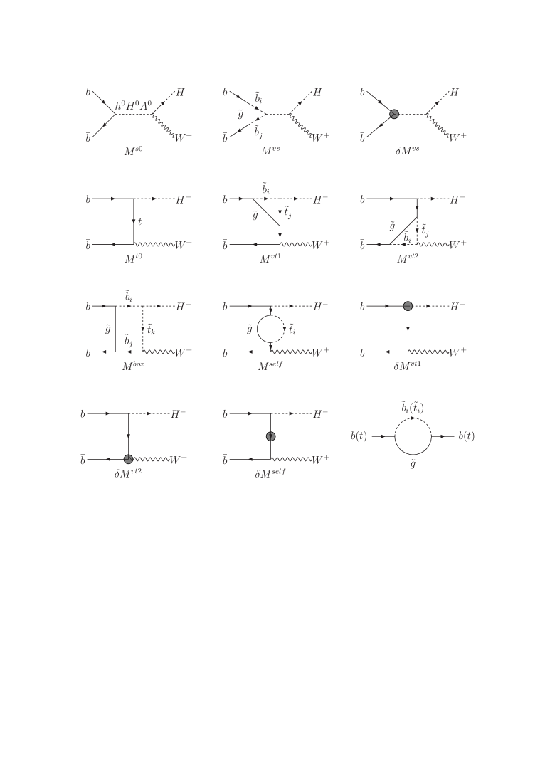
Figure 1: Feynmann diagrams for the subprocess $b\bar{b}\rightarrow W^{+}H^{-}$. Born diagrams: $M^{s0}$ ,$M^{t0}$; Virtual correction diagrams: $M^{vs},M^{vt1},M^{vt2},M^{box},M^{self}$; Counter-term diagrams: $\delta M^{vs},\delta M^{vt1},\delta M^{vt2},\delta M^{self}$.

After calculating the self-energy diagram in Fig. 1, we obtain the explicit expressions of all the renormalization constants as follows:

$$\delta m_{q}= -\frac{\alpha_{s}}{3\pi}\big{[}m_{q}[B_{1}(m^{2}_{q},m^{2}_{\tilde{g}},m^{2}_{\tilde{q}_{1}})+B_{1}(m^{2}_{q},m^{2}_{\tilde{g}},m^{2}_{\tilde{q}_{2}})]+m_{\tilde{g}}\sin 2\theta_{\tilde{q}}[B_{0}(m^{2}_{q},m^{2}_{\tilde{g}},m^{2}_{\tilde{q}_{1}})$$

$$-B_{0}(m^{2}_{q},m^{2}_{\tilde{g}},m^{2}_{\tilde{q}_{2}})]\big{]},$$

$$\delta Z^{q}_{L}= \frac{2\alpha_{s}}{3\pi}\big{[}\cos^{2}\theta_{\tilde{q}}B^{1}_{1}+\sin^{2}\theta_{\tilde{q}}B^{2}_{1}+m^{2}_{q}[\dot{B}^{1}_{1}+\dot{B}^{2}_{1}+\frac{m_{\tilde{g}}}{m_{q}}\sin 2\theta_{\tilde{q}}(\dot{B}^{1}_{0}-\dot{B}^{2}_{0})]\big{]},$$ (5)

$$\delta Z^{q}_{R}= \frac{2\alpha_{s}}{3\pi}\big{[}\sin^{2}\theta_{\tilde{q}}B^{1}_{1}+\cos^{2}\theta_{\tilde{q}}B^{2}_{1}+m^{2}_{q}[\dot{B}^{1}_{1}+\dot{B}^{2}_{1}+\frac{m_{\tilde{g}}}{m_{q}}\sin 2\theta_{\tilde{q}}(\dot{B}^{1}_{0}-\dot{B}^{2}_{0})]\big{]},$$ (6)

where $B^{i}_{m}=B_{m}(m^{2}_{q},m^{2}_{\tilde{g}},m^{2}_{\tilde{q}_{i}}),\dot{B}^{i}_{m}=\dot{B}_{m}(m^{2}_{q},m^{2}_{\tilde{g}},m^{2}_{\tilde{q}_{i}})$ with $q=b,\,t$ are the two-point integrals denner , $m_{\tilde{q}_{i}}$ are the squark masses, $m_{\tilde{g}}$ is the gluino mass, and $\theta_{\tilde{q}}$ is the mixing angle of the squarks.

The Feynman diagrams for the subprocess $b\bar{b}\rightarrow H^{-}W^{+}$, which include the SUSY-QCD corrections to the process, are shown in Fig.1 and its renomalized amplitude can be written as

$$M^{ren.}=M^{0}+M^{vir.}+\delta M^{count.}.$$ (7)

Here $M^{0}$ is the tree-level amplitude, which is given by summing over the s- and t-channel amplitudes:

$$M^{0}=M^{s0}+M^{t0},$$ (8)

with

$$M^{s0}=\frac{2\pi\alpha m_{b}}{m_{w}\sin^{2}\theta_{w}}\bigg{[}S_{b}(A_{4}+A_{3})+P_{b}(A_{4}-A_{3})\bigg{]},$$ (9)

$$M^{t0}=\frac{2\pi\alpha}{m_{w}\sin^{2}\theta_{w}}\frac{1}{t-m_{t}^{2}}\big{[}m^{2}_{t}\cot\beta A_{10}+m_{b}\tan\beta(A_{11}-2A_{3})\big{]},$$ (10)

where $S_{b}$ and $P_{b}$ are defined by

$$S_{b}=\frac{1}{\cos\beta}\left[-\frac{\sin\alpha\cos(\alpha-\beta)}{s-m^{2}_{h^{0}}}+\frac{\cos\alpha\sin(\alpha-\beta)}{s-m^{2}_{H^{0}}}\right],$$ (11)

$$P_{b}=\frac{1}{\cos\beta}\frac{\sin\beta}{s-m^{2}_{A^{0}}},$$ (12)

$A_{i}$ are reduced standard matrix elements, which are given by

$$A_{1}=\bar{v}(p_{2})P_{R}u(p_{1})p_{1}\cdot\varepsilon(p_{4}),$$

$$A_{2}=\bar{v}(p_{2})P_{L}u(p_{1})p_{1}\cdot\varepsilon(p_{4}),$$

$$A_{3}=\bar{v}(p_{2})P_{R}u(p_{1})p_{3}\cdot\varepsilon(p_{4}),$$

$$A_{4}=\bar{v}(p_{2})P_{L}u(p_{1})p_{3}\cdot\varepsilon(p_{4}),$$ (13)

$$A_{5}=\bar{v}(p_{2})\not p_{3}P_{R}u(p_{1})p_{1}\cdot\varepsilon(p_{4}),$$

$$A_{6}=\bar{v}(p_{2})\not p_{3}P_{L}u(p_{1})p_{1}\cdot\varepsilon(p_{4}),$$

$$A_{7}=\bar{v}(p_{2})\not p_{3}P_{R}u(p_{1})p_{3}\cdot\varepsilon(p_{4}),$$

$$A_{8}=\bar{v}(p_{2})\not p_{3}P_{L}u(p_{1})p_{3}\cdot\varepsilon(p_{4}),$$

$$A_{9}=\bar{v}(p_{2})\not\varepsilon(p_{4})P_{R}u(p_{1}),$$

$$A_{10}=\bar{v}(p_{2})\not\varepsilon(p_{4})P_{L}u(p_{1}),$$

$$A_{11}=\bar{v}(p_{2})\not p_{3}\not\varepsilon(p_{4})P_{R}u(p_{1}),$$

$$A_{12}=\bar{v}(p_{2})\not p_{3}\not\varepsilon(p_{4})P_{L}u(p_{1}),$$

and $M^{vir.}$ contains the radiative corrections from the one-loop self-energy, vertex, and box diagrams, of which corresponding amplitudes are shown in Appendix B. The counter-term $\delta M^{count.}$ contains the contributions from the corresponding vertex and self-energy counterterms, which are given by

$$\delta M^{vs}= M^{s0}(\frac{\delta m_{b}}{m_{b}}+\frac{1}{2}\delta Z^{b}_{R}+\frac{1}{2}\delta Z^{b}_{L}),$$ (14)

$$\delta M^{vt1}= \frac{2\pi\alpha}{m_{w}\sin^{2}\theta_{w}}\frac{1}{t-m_{t}^{2}}\big{[}m^{2}_{t}\cot\beta(\frac{\delta m_{t}}{m_{t}}+\frac{1}{2}\delta Z^{t}_{R}+\frac{1}{2}\delta Z^{b}_{L})A_{10}$$ (15)

$$+m_{b}\tan\beta(\frac{\delta m_{b}}{m_{b}}+\frac{1}{2}\delta Z^{t}_{L}+\frac{1}{2}\delta Z^{b}_{R})(A_{11}-2A_{3})\big{]},$$

$$\delta M^{vt2}= M^{t0}(\frac{1}{2}\delta Z^{b}_{L}+\frac{1}{2}\delta Z^{t}_{L}),$$ (16)

$$\delta M^{self}= \frac{2\pi\alpha}{m_{w}\sin^{2}\theta_{w}}\frac{1}{t-m^{2}_{t}}\bigg{[}m^{2}_{t}\cot\beta(\frac{\delta m_{t}}{m_{t}}+\frac{1}{2}\delta Z^{t}_{L}+\frac{1}{2}\delta Z^{t}_{R})A_{10}$$ (17)

$$+m_{b}\tan\beta(\delta Z^{t}_{L}+\frac{2m^{2}_{t}}{t-m^{2}_{t}}\frac{\delta m_{t}}{m_{t}})(A_{11}-2A_{3})\bigg{]}.$$

The partonic cross section can be written as following:

$$\hat{\sigma}=\int^{1}_{-1}\mbox{d}z\frac{1}{32\pi s^{2}}\lambda^{1/2}\overline{\left|M^{ren.}\right|^{2}}=\int^{t_{+}}_{t_{-}}\mbox{d}t\frac{1}{16\pi s^{2}}\overline{\left|M^{ren.}\right|^{2}},$$ (18)

where $\lambda\equiv(s+m^{2}_{W}-m^{2}_{H^{-}})^{2}-4sm^{2}_{W}$, $t_{\pm}=\frac{1}{2}[m^{2}_{H^{-}}+m_{W}^{2}-s\pm\lambda^{1/2}],$ and $\overline{\left|M^{ren.}\right|^{2}}$ is the renormalized amplitude squared, which is given by

$$\overline{\left|M^{ren.}\right|^{2}}=\overline{\sum}\left|M^{0}\right|^{2}+2\mbox{Re}\overline{\sum}M^{0}[M^{vir.}+\delta M^{count.}]^{\dagger},$$ (19)

where the colors and spins of the outgoing particles have been summed over, and the colors and spins of incoming ones have been averaged over. We notice that the color average factors of LO and NLO amplitudes squared are different: $\frac{1}{3}\times\frac{1}{3}\mbox{Tr}{\openone}=\frac{1}{3}$ for LO amplitudes, and $\frac{1}{3}\times\frac{1}{3}\mbox{Tr}(\mbox{T}^{a}\mbox{T}^{a})=\frac{4}{9}$ for NLO ones. The both spin average factors are the same $\frac{1}{2}\times\frac{1}{2}=\frac{1}{4}$.

The total cross section at the LHC is obtained by convoluting the partonic cross section with the parton distribution functions (PDFs) $G_{b,\bar{b}/p}$ in the proton:

$$\sigma=\int^{1}_{\tau_{0}}dx_{1}\int^{1}_{\tau_{0}/x_{1}}dx_{2}[G_{b/p}(x_{1},\mu_{f})G_{\bar{b}/p}(x_{2},\mu_{f})+(x_{1}\leftrightarrow x_{2})]\hat{\sigma}(\tau S),$$ (20)

where $\mu_{f}$ is the factorization scale and $S=(P_{1}+P_{2})^{2}$, $P_{1}$ and $P_{2}$ are the four-momentum of the incident hadrons, $\tau_{0}=\frac{(m_{W}+m_{H^{-}})^{2}}{S}$, $\tau=x_{1}x_{2}$, and $x_{1}$ and $x_{2}$ are the longitudinal momentum fractions of initial partons in the hadrons.

In the following, we present the differential cross sections in the transverse momentum $p_{T}$ and rapidity Y of the W-boson, and the invariant mass $M_{W^{+}H^{-}}$, respectively. In the center-of-mass frame of initial hadrons, $P_{1}=\sqrt{S}/2(1,0,0,1)$ and $P_{2}=\sqrt{S}/2(1,0,0,-1)$, and the four-momentum of W-boson is defined by $p_{4}=(E,\mathbf{p_{T}},p_{L})$. The transverse momentum $p_{T}$ and the rapidity Y of W-boson, and the invariant mass $M_{W^{+}H^{-}}$ are defined by

$$p_{T}^{2} = (E-p_{L})(E+p_{L})-m_{W}^{2}=\frac{(m_{W}^{2}-t)(m^{2}_{W}-u)}{s}-m_{W}^{2},$$ (21)

$$Y = \frac{1}{2}\log\left(\frac{E+p_{L}}{E-p_{L}}\right),$$ (22)

and

$$M^{2}_{W^{+}H^{-}}=(p_{3}+p_{4})^{2}=(p_{1}+p_{2})^{2}=s=x_{1}x_{2}S,$$ (23)

respectively.

The three differential cross sections are thus given by

$$\frac{\mbox{d}{\sigma}}{\mbox{d}p_{T}}=\int^{1}_{\tau_{0}}dx_{1}\int^{1}_{\tau_{0}/x_{1}}dx_{2}[G_{b/p}(x_{1},\mu_{f})G_{\bar{b}/p}(x_{2},\mu_{f})+(x_{1}\leftrightarrow x_{2})]\frac{\mbox{d}\hat{\sigma}}{\mbox{d}p_{T}},$$ (24)

$$\frac{\mbox{d}{\sigma}}{\mbox{d}Y}=\int^{1}_{\tau_{0}}dx_{1}\int^{1}_{\tau_{0}/x_{1}}dx_{2}[G_{b/p}(x_{1},\mu_{f})G_{\bar{b}/p}(x_{2},\mu_{f})+(x_{1}\leftrightarrow x_{2})]\frac{\mbox{d}\hat{\sigma}}{\mbox{d}Y},$$ (25)

and

$$\frac{\mbox{d}{\sigma}}{\mbox{d}M_{W^{+}H^{-}}}=\int^{1}_{\tau_{0}}\frac{\mbox{d}x_{1}}{x_{1}}\frac{2M_{W^{+}H^{-}}}{\tau S}[G_{b/p}(x_{1},\mu_{f})G_{\bar{b}/p}(x_{2},\mu_{f})+(x_{1}\leftrightarrow x_{2})]\mbox{d}\hat{\sigma},$$ (26)

respectively,
with

$$\frac{\mbox{d}\hat{\sigma}}{\mbox{d}p_{T}}=\frac{1}{32\pi s^{2}}\lambda^{1/2}\lvert\frac{4sp_{T}}{z\lambda}\rvert\overline{\left|M^{ren.}\right|^{2}},$$ (27)

and

$$\frac{\mbox{d}\hat{\sigma}}{\mbox{d}Y}=\frac{1}{16\pi s^{2}}\lvert(s+m_{W}^{2}-m^{2}_{H^{-}})\frac{2u}{(u+1)^{2}}\rvert\overline{\left|M^{ren.}\right|^{2}},$$ (28)

where $z=\pm\sqrt{1-\frac{4sp^{2}_{T}}{\lambda}}$ and $u=\frac{x_{1}}{x_{2}}e^{-2Y}$.

.3 Numerical Results and Conclusions

In this section, we present the numerical results for the SUSY-QCD corrections to $W^{+}H^{-}$ associated production at the LHC. In our numerical calculations, we used the following set of the SM parameterssmparameter :

$$\alpha_{ew}(m_{W})=1/128,\ m_{W}=80.419\,{\rm\,GeV},\ m_{Z}=91.1882\,{\rm\,GeV}\,,$$

$$m_{b}=4.25\,{\rm\,GeV},m_{t}=178\,{\rm\,GeV},\ \alpha_{s}(M_{Z})=0.118.$$ (29)

The running QCD coupling $\alpha_{s}(Q)$ is evaluated at the two-loop order 2loopalfs , and the CTEQ6M PDFs pdf are used throughout this paper either at the LO or NLO. For simplicity, we neglect the b-quark mass but keep it in the couplings. Moreover, in order to improve the perturbative calculations, we took the running mass $m_{b}(Q)$ and $m_{t}(Q)$ evaluated the NLO formulamrunning :

$$m_{b}(Q)=U_{6}(Q,m_{t})U_{5}(m_{t},m_{b})m_{b}(m_{b})\,,$$ (30)

$$m_{t}(Q)=U_{6}(Q,m_{t})m_{t}(m_{t})\,,$$ (31)

where the evolution factor $U_{f}$ is

$$U_{f}(Q_{2},Q_{1})=\bigg{(}\frac{\alpha_{s}(Q_{2})}{\alpha_{s}(Q_{1})}\bigg{)}^{d^{(f)}}\bigg{[}1+\frac{\alpha_{s}(Q_{1})-\alpha_{s}(Q_{2})}{4\pi}J^{(f)}\bigg{]},$$

$$d^{(f)}=\frac{12}{33-2f},\hskip 28.45274ptJ^{(f)}=-\frac{8982-504f+40f^{2}}{3(33-2f)^{2}}\,,$$ (32)

and $f$ is the number of the active light quarks.

In addition, to also improve the perturbation calculations, we made the following SUSY replacements in the tree-level couplingsmrunning ; mtrunning

$$m_{q}(Q)\ \ \rightarrow\ \ \frac{m_{q}(Q)}{1+\Delta m_{q}}\,\,\,\,(q=b,t),$$ (33)

$$\Delta m_{b}= \frac{2\alpha_{s}}{3\pi}M_{\tilde{g}}\mu\tan\beta I(m_{\tilde{b}_{1}},m_{\tilde{b}_{2}},M_{\tilde{g}})\,,$$ (34)

$$\Delta m_{t}= -\frac{\alpha_{s}}{3\pi}\{\bar{B}_{1}(0,m^{2}_{\tilde{g}},m^{2}_{\tilde{t}_{1}})+\bar{B}_{1}(0,m^{2}_{\tilde{g}},m^{2}_{\tilde{t}_{2}})$$ (35)

$$-\sin 2\theta_{t}(\frac{m_{\tilde{g}}}{m_{t}})[\bar{B}_{0}(0,m^{2}_{\tilde{g}},m^{2}_{\tilde{t}_{1}})-\bar{B}_{0}(0,m^{2}_{\tilde{g}},m^{2}_{\tilde{t}_{1}})]\},$$

where

$$I(a,b,c)=\frac{1}{(a^{2}-b^{2})(b^{2}-c^{2})(a^{2}-c^{2})}(a^{2}b^{2}\log\frac{a^{2}}{b^{2}}+b^{2}c^{2}\log\frac{b^{2}}{c^{2}}+c^{2}a^{2}\log\frac{c^{2}}{a^{2}})\,,$$ (36)

$$\bar{B}_{1}=B_{1}+\Delta/2,\bar{B}_{0}=B_{0}-\Delta\,\,\,(\Delta=1/\epsilon-\gamma+\ln 4\pi).$$

It is necessary to avoid double counting by subtracting these SUSY-QCD corrections from the renormalization constant. As for the renormalization and factorization scales, we always chose $\mu_{r}=\mu_{f}=(m_{W}+m_{H^{-}})/2$.

The values of the MSSM parameters taken in our numerical calculations were constrained within the minimal supergravity scenario (mSUGRA)msugra , in which there are only five free input parameters at the grand unification where $m_{1/2},\,m_{0},\,A_{0},\mbox{tan}\beta$ and the sign of $\mu$, where $m_{1/2},\,m_{0},\,A_{0}$ are, respectively, the universal gaugino mass, scalar mass, and the trilinear soft breaking parameter in the superpotential. Given these parameters, all the MSSM parameters at the weak scale are determined in the mSUGRA scenario by using the the program package SUSPECT 2.3suspect .

Figs. 2 and  3 show the total cross sections and the relative corrections as functions of $m_{1/2}$ (or $m_{\tilde{g}}$) for $\mu<0$ and tan$\beta$=4,  10,  and 40, respectively. The total cross sections decrease with the increasing of $m_{1/2}$ as expected. For small tan$\beta$, the relative SUSY-QCD corrections are small and can be negligible. For large tan$\beta(\sim 40)$, the relative SUSY-QCD corrections become large and increase when $m_{\tilde{g}}$ increases. Indeed, in our numerical calculations, the dependence of the total cross sections on $m_{\tilde{g}}$ is got through varying $m_{1/2}$. And when $m_{1/2}$ increases, both $m_{\tilde{g}}$ and $m_{H^{\pm}}$ increase. The increase of $m_{H^{\pm}}$ decreases the phase spaces of the LO total cross sections, and the magnitudes of the SUSY-QCD corrections also become smaller with the increasing of both $m_{\tilde{g}}$ and $m_{H^{\pm}}$. But the decrease rate of the LO total cross sections is larger than the one of the SUSY-QCD corrections, so the relative corrections increase with the increasing of $m_{1/2}$ as shown in Fig. 3.

In Figs. 4 and  5 we present the LO and the SUSY-QCD corrected total cross sections, and the SUSY-QCD corrections as functions of $m_{H^{-}}$ for $\mu<0$ and $\tan\beta=4,10,40$, respectively. Both the LO and the SUSY-QCD corrected cross sections decrease when $m_{H^{-}}$ increases, and for large $\tan\beta$, the corrections in general enhance the total cross sections for $\mu<0$. For large $\mbox{tan}\beta(\sim 40)$ the total cross sections become significant and can reach several tens fb, and even one hundred fb when $m_{H^{-}}<200\mbox{\,GeV}$, while for small $\mbox{tan}\beta$ the total cross sections are about serval fb and can be neglected. For $\mbox{tan}\beta=40$, in general, the corrections can exceed $4\%$, and even they can reach $10\%$ when $m_{H^{-}}\sim 150\mbox{\,GeV}$. For $\tan\beta=4,10$, the magnitude of the corrections are always smaller than $2\%$. Note that for $\mu<0$ and $\tan\beta=4,10$, the mass of the charged Higgs can not be smaller than about $250$ GeV, just as shown by the curves in these figures.

Figs. 6 and  7 show the cross sections and the relative corrections as functions of tan$\beta$, assuming $m_{0}=160,\,400$ GeV, and the sign of $\mu=\pm 1$, respectively. From these figures, we find that the total cross sections for the case of $\mu>0$ are obviously smaller than those for $\mu<0$, and that when tan$\beta$ becomes larger the SUSY-QCD corrections increase the total cross sections for $\mu<0$, while decrease for $\mu>0$. For small $\tan\beta$, the variations of these curves are not monotonic because the contributions from the Yukawa coupling $\mbox{H}^{-}t\bar{b}$ contain not only the terms proportional to tan$\beta$ but also the ones to cot$\beta$.

Above results for representative values of $m_{H^{-}}$ and tan$\beta$ can be summarized in table 1.

$m_{H^{+}}$ GeV	tan$\beta$=4	tan$\beta$=10	tan$\beta$=40
150	$-$	$-$	$\sim$ 10 $\%$
300	$\sim 0.2\%$	$\sim-0.2\%$	$\sim 5\%$
500	$\sim 0.8\%$	$\sim-0.7\%$	$\sim 4\%$

Table 1: The SUSY-QCD corrections for tan$\beta$=4,  10, 40 and $m_{H^{-}}=150,\,300,\,500$ GeV, respectively, assuming $A_{0}=250$ GeV, $m_{1/2}=180$ GeV, $\mu<0$.

In Figs.8-10, we display the differential cross sections as functions of the transverse momentum $p_{T}$, the rapidity Y of the W-boson, and the invariant mass $M_{W^{+}H^{-}}$, which are given by Eqs.24, 25, and 26, respectively. We find that the SUSY-QCD corrections increase the LO differential cross sections for $\mu<0$, and decrease ones for $\mu>0$. The differential cross sections can reach the maximum value at $p_{T}=55$ GeV and 70  GeV, $\mbox{M}_{W^{+}H^{-}}=310$ and 370  GeV for $\mu<0$ and $\mu>0$, respectively. The differential cross sections in the rapidity of W-boson is symmetric about the axis of Y=0 as expected.

Finally, we compare the SUSY-QCD corrections with the ${\cal O}(\alpha_{ew}m^{2}_{t(b)}/m^{2}_{W})$ and ${\cal O}(\alpha_{ew}m^{4}_{t(b)}/m^{4}_{W})$ SUSY-EW and the ${\cal O}(\alpha_{s})$ QCD corrections. We notice that the QCD and the SUSY-EW corrections are large and dominate over the SUSY-QCD ones for small $\tan\beta$. When $\tan\beta$ becomes large the SUSY-QCD corrections increase. Although the magnitudes of the SUSY-QCD corrections are still smaller than the ones of the ${\cal O}(\alpha_{s})$ QCD corrections, they can exceed $10\%$, which are larger than those of the SUSY-EW corrections. Especially, for $\mu<0$, the sign of SUSY-QCD corrections is opposite to the ones of the other two corrections, thus the SUSY-QCD corrections can cancel with the SUSY-EW and QCD corrections to some extent. In order to compare these corrections clearly, we show the three corrections to the process $b\bar{b}\rightarrow W^{-}H^{+}$ in some typical parameter space in the table 2.

In conclusion, we have calculated the SUSY-QCD corrections to the total cross sections for the $W^{+}H^{-}$ associated production in the MSSM at the LHC. The SUSY-QCD corrections can increase and decrease the total cross sections depending on the choice of the SUSY parameters. For $\mu<0$, the SUSY-QCD corrections can increase the total cross sections significantly, especially for large tan$\beta$, which have the opposite sign with respect to the QCD and the SUSY-EW corrections, and cancel with them to some extent.

	${\cal O}(\alpha_{ew}m^{2}_{t(b)}/m^{2}_{W})$ and ${\cal O}(\alpha_{ew}m^{4}_{t(b)}/m^{4}_{W})$	${\cal O}(\alpha_{s})$ QCD	SUSY-QCD
tan$\beta$	SUSY-EW corrections bbsusyew	corrections bbqcd	corrections
4	$\sim-14\%$	$\sim-32\%$	$\sim$ 0
40	$\sim-1\%$	$\sim-17\%$	$\sim 8\%$

Table 2: Comparison of the SUSY-QCD corrections with the QCD and SUSY-EW ones, for tan$\beta=4,\,40$, respectively, assuming $m_{H^{-}}=200$GeV and $\mu<0$.

I Acknowledgements

This work was supported in part by the National Natural Science Foundation of China, under grant Nos.10421003 and 10575001, and the Key Grant Project of Chinese Ministry of Education, under grant NO.305001.

Appendix A

In this Appendix, we will list the relevant pieces of SUSY Lagranian. The Yukawa couplings of Higgs and quarks are given by

$${\cal L}_{(h^{0},H^{0},A^{0})\bar{b}b}=\frac{gm_{b}}{2m_{w}\cos\beta}\sin\alpha h^{0}\bar{b}b-\frac{gm_{b}}{2m_{w}\cos\beta}\cos\alpha H^{0}\bar{b}b+i\frac{gm_{b}}{2m_{w}}\tan\beta A^{0}\bar{b}\gamma_{5}b,$$

$${\cal L}_{H^{-}\bar{t}b}=\frac{g}{\sqrt{2}m_{w}}H^{+}\bar{t}(m_{t}\cot\beta P_{L}+m_{b}\tan\beta P_{R})b+h.c.,$$

where $P_{L,R}=(1\mp\gamma_{5})/2$ are the chiral projector operators, tan$\beta=v_{u}/v_{d}$ is the ratio of vaccum expectation values of the two Higgs doublets.

The trilinear couplings of Higgs bosons and W-boson are given by

$${\cal L}_{(h^{0},H^{0},A^{0})H^{-}W^{+}}=i\frac{g}{2}\big{[}\cos(\alpha-\beta)h^{0}\overleftrightarrow{\partial_{\mu}}H^{-}+\sin(\alpha-\beta)H^{0}\overleftrightarrow{\partial_{\mu}}H^{-}+iA^{0}\overleftrightarrow{\partial_{\mu}}H^{-}\big{]}W^{+\mu}+h.c.$$

The squarks couplings to gluino, W-boson and Higgs are given by

$${\cal L}_{\tilde{g}q\tilde{q}}=-\sqrt{2}T^{a}[\bar{q}(\mbox{R}^{\tilde{q}}_{i1}P_{R}-\mbox{R}^{\tilde{q}}_{i2}P_{L})\tilde{g}\tilde{q}_{i}+\bar{\tilde{g}}(\mbox{R}^{\tilde{q}}_{i1}P_{R}-\mbox{R}^{\tilde{q}}_{i2}P_{L})q\,\tilde{q}^{\ast}_{i}],$$

$${\cal L}_{\tilde{t}^{\ast}\tilde{b}W}=i\frac{g}{\sqrt{2}}(\mbox{R}^{\tilde{b}}_{i1}\mbox{R}^{\tilde{t}}_{j1}W^{+\mu}\tilde{t}^{\ast}_{j}\overleftrightarrow{\partial}_{\mu}\tilde{b}_{i}+\mbox{R}^{\tilde{t}}_{i1}\mbox{R}^{\tilde{b}}_{j1}W^{-\mu}\tilde{b}^{\ast}_{j}\overleftrightarrow{\partial}_{\mu}\tilde{t}_{i}),$$

$${\cal L}_{H^{k}\tilde{b}^{\ast}\tilde{b}}=gG^{k}_{ij}H^{k}\tilde{b}^{\ast}_{j}\tilde{b}_{i}\hskip 85.35826pt(H^{k}=h^{0},H^{0},A^{0}),$$

$${\cal L}_{H^{k}\tilde{t}^{\ast}\tilde{b}}=\frac{g}{\sqrt{2}m_{w}}G^{k}_{ij}H^{k}\tilde{t}^{\ast}_{j}\tilde{b}_{i}+h.c.\hskip 56.9055pt(H^{k}=H^{-}),$$

where

$$\hskip 85.35826ptG^{k}_{ij}=[\mbox{R}^{\tilde{b}}\hat{G}^{k}\mbox{R}^{\tilde{b}T}]_{ij},$$

$$\hat{G}^{h^{0}}=\left(\begin{array}[]{cc}-\frac{m_{z}}{\cos\theta_{w}}(\frac{1}{2}-\frac{1}{3}\sin^{2}\theta_{w})\sin(\alpha+\beta)+\frac{m^{2}_{b}}{2m_{w}\cos\beta}\sin\alpha&\frac{m_{b}}{2m_{w}\cos\beta}(A_{b}\sin\alpha+\mu\cos\alpha)\\ \frac{m_{b}}{2m_{w}\cos\beta}(A_{b}\sin\alpha+\mu\cos\alpha)&-\frac{1}{3}\frac{m_{z}}{\cos\theta_{w}}\sin^{2}\theta_{w}\sin(\alpha+\beta)+\frac{m^{2}_{b}}{2m_{w}\cos\beta}\sin\alpha\end{array}\right),$$

$$\hat{G}^{H^{0}}=\left(\begin{array}[]{cc}\frac{m_{z}}{\cos\theta_{w}}(\frac{1}{2}-\frac{1}{3}\sin^{2}\theta_{w})\cos(\alpha+\beta)-\frac{m^{2}_{b}}{2m_{w}\cos\beta}\sin\alpha&-\frac{m_{b}}{2m_{w}\cos\beta}(A_{b}\cos\alpha-\mu\sin\alpha)\\ -\frac{m_{b}}{2m_{w}\cos\beta}(A_{b}\cos\alpha-\mu\sin\alpha)&\frac{1}{3}\frac{m_{z}}{\cos\theta_{w}}\sin^{2}\theta_{w}\sin(\alpha+\beta)-\frac{m^{2}_{b}}{2m_{w}\cos\beta}\sin\alpha\end{array}\right),$$

$$\hat{G}^{A^{0}}=\frac{im_{b}}{2m_{w}}\left(\begin{array}[]{cc}0&-(A_{b}\tan\beta+\mu)\\ (A_{b}\tan\beta+\mu)&0\end{array}\right),$$

$$\hat{G}^{H^{-}}=\left(\begin{array}[]{cc}m^{2}_{b}\tan\beta+m^{2}_{t}\cot\beta-m^{2}_{w}\sin 2\beta&m_{b}(A_{b}\tan\beta+\mu)\\ m_{t}(A_{t}\cot\beta+\mu)&\frac{2m_{t}m_{b}}{\sin 2\beta}\end{array}\right),$$

where $R^{\tilde{q}}$ is a $2\times 2$ matrix shown as below, which is defined to transform the squark current eigenstates to the mass eigenstates squarkrotation :

$$\left(\begin{array}[]{c}\tilde{q}_{1}\\ \tilde{q}_{2}\end{array}\right)=R^{\tilde{q}}\left(\begin{array}[]{c}\tilde{q}_{L}\\ \tilde{q}_{R}\end{array}\right),\ \ \ \ \ R^{\tilde{q}}=\left(\begin{array}[]{cc}\cos\theta_{\tilde{q}}&\sin\theta_{\tilde{q}}\\ -\sin\theta_{\tilde{q}}&\cos\theta_{\tilde{q}}\end{array}\right),$$

with $0\leq\theta_{\tilde{b}}<\pi$, by convention. Correspondingly, the mass eigenvalues $m_{\tilde{q}_{1}}$ and $m_{\tilde{q}_{2}}$ (with $m_{\tilde{q}_{1}}\leq m_{\tilde{q}_{2}}$) are given by

$$\left(\begin{array}[]{cc}m_{\tilde{q}_{1}}^{2}&0\\ 0&m_{\tilde{q}_{2}}^{2}\end{array}\right)=R^{\tilde{q}}M_{\tilde{q}}^{2}(R^{\tilde{q}})^{\dagger},\ \ \ \ \ M_{\tilde{q}}^{2}=\left(\begin{array}[]{cc}m_{\tilde{q}_{L}}^{2}&a_{q}m_{q}\\ a_{q}m_{q}&m_{\tilde{q}_{R}}^{2}\end{array}\right),$$

with

$$m^{2}_{\tilde{q}_{L}} = M^{2}_{\tilde{Q}}+m_{q}^{2}+m_{Z}^{2}\cos 2\beta(I_{3L}^{q}-e_{q}\sin^{2}\theta_{W}),$$

$$m^{2}_{\tilde{q}_{R}} = M^{2}_{\tilde{D}}+m_{q}^{2}+m_{Z}^{2}\cos 2\beta e_{q}\sin^{2}\theta_{W},$$

$$a_{q} = A_{q}-\mu\tan\beta.$$

Here, $M_{\tilde{q}}^{2}$ is the squark mass matrix. $M_{\tilde{Q},\tilde{D}}$ and $A_{q}$ are soft SUSY breaking parameters and $\mu$ is the higgsino mass parameter. $I_{3L}^{q}$ and $e_{q}$ are the third component of the weak isospin and the electric charge of the quark $q$, respectively.

Appendix B

In this Appendix, we will list the explicit expressions of the vertex, box and self-energy diagrams. For simplicity, we introduce the following abbreviations for the Passarino-Veltman two-point integrals $B_{i}$, tree-point integrals $C_{i(j)}$ and four-point integrals $D_{ij}$, which are defined similarly to Ref. denner except that we take internal masses squared as arguments:

$$B_{i}=B_{i}(t,m^{2}_{\tilde{g}},m^{2}_{\tilde{t}_{i}}),$$

$$C^{a}_{0}=C_{0}(0,s,0,m^{2}_{\tilde{g}},m^{2}_{\tilde{b}_{i}},m^{2}_{\tilde{b}_{j}}),$$

$$C^{b}_{i}=C_{i}(0,m^{2}_{H^{-}},t,m^{2}_{\tilde{g}},m^{2}_{\tilde{b}_{i}},m^{2}_{\tilde{t}_{j}}),$$

$$C^{d}_{i(j)}=C_{i(j)}(0,m^{2}_{w},t,m^{2}_{\tilde{g}},m^{2}_{\tilde{b}_{i}},m^{2}_{\tilde{t}_{j}}),$$

$$D_{ij}=D_{ij}(0,s,m^{2}_{w},t,0,m^{2}_{H^{-}},m^{2}_{\tilde{g}},m^{2}_{\tilde{b}_{i}},m^{2}_{\tilde{b}_{j}},m^{2}_{\tilde{t}_{k}}).$$

The explicit expressions of the corresponding self-energy,vertex and box diagrams are given by

$${\cal M}^{vs}=-\frac{2\alpha\alpha_{s}m_{\tilde{g}}}{\sin^{2}\theta_{w}}\bigg{[}\frac{G^{h^{0}}_{ij}\cos(\alpha-\beta)}{s-m^{2}_{h^{0}}}+\frac{G^{H^{0}}_{ij}\sin(\alpha-\beta)}{s-m^{2}_{H^{0}}}+\frac{G^{A^{0}}_{ij}}{s-m^{2}_{A^{0}}}\bigg{]}\big{[}\mbox{R}^{\tilde{b}}_{i2}\mbox{R}^{\tilde{b}}_{j1}A_{3}+\mbox{R}^{\tilde{b}}_{i1}\mbox{R}^{\tilde{b}}_{j2}A_{4}\big{]}C^{a}_{0},$$

$${\cal M}^{vt1}=\frac{\alpha\alpha_{s}}{\sin^{2}\theta_{w}m_{w}}\frac{G^{H^{-}}_{ij}}{t-m^{2}_{t}}\bigg{[}\big{[}\mbox{R}^{\tilde{b}}_{i1}\mbox{R}^{\tilde{t}}_{j1}tC^{b}_{2}+\mbox{R}^{\tilde{b}}_{i1}\mbox{R}^{\tilde{t}}_{j2}m_{\tilde{g}}m_{t}C^{b}_{0}\big{]}A_{10}$$

$$\hskip 42.67912pt+\big{[}\mbox{R}^{\tilde{b}}_{i2}\mbox{R}^{\tilde{t}}_{j1}m_{\tilde{g}}C^{b}_{0}+\mbox{R}^{\tilde{b}}_{i2}\mbox{R}^{\tilde{t}}_{j2}m_{t}C^{b}_{2}\big{]}\big{[}A_{11}-2A_{3}\big{]}\bigg{]},$$

$${\cal M}^{vt2}=\frac{2\alpha\alpha_{s}}{\sin^{2}\theta_{w}m_{w}}\frac{\mbox{R}^{\tilde{b}}_{i1}\mbox{R}^{\tilde{t}}_{j1}}{t-m^{2}_{t}}\bigg{[}\mbox{R}^{\tilde{b}}_{i1}\mbox{R}^{\tilde{t}}_{j1}\big{[}m^{2}_{t}\cot\beta[C^{d}_{00}A_{10}+C^{d}_{12}(A_{6}-A_{8})]+m_{b}\tan\beta[C^{d}_{00}(A_{11}-2A_{3})$$

$$\hskip 42.67912pt+tC^{d}_{12}(A_{3}-A_{1})]\big{]}+\mbox{R}^{\tilde{b}}_{i1}\mbox{R}^{\tilde{t}}_{j2}m_{\tilde{g}}m_{t}C^{d}_{1}[\cot\beta(A_{6}-A_{8})+m_{b}\tan\beta(A_{3}-A_{1})]$$

$$\hskip 42.67912pt-\mbox{R}^{\tilde{b}}_{i2}\mbox{R}^{\tilde{t}}_{j1}m_{\tilde{g}}C^{d}_{1}\big{[}m^{2}_{t}\cot\beta(A_{2}-A_{4})+m_{b}\tan\beta(A_{7}-A_{5})\big{]}$$

$$\hskip 42.67912pt+\mbox{R}^{\tilde{b}}_{i2}\mbox{R}^{\tilde{t}}_{j2}m_{t}\big{[}\cot\beta[C^{d}_{00}(A_{12}-2A_{4})+tC^{d}_{12}(A_{4}-A_{2})]$$

$$\hskip 42.67912pt+m_{b}\tan\beta[C^{d}_{12}(A_{5}-A_{7})+C^{d}_{00}A_{9}]\big{]}\bigg{]},$$

$${\cal M}^{box}=\frac{2\alpha\alpha_{s}}{\sin^{2}\theta_{w}m_{w}}\mbox{R}^{\tilde{b}}_{j1}\mbox{R}^{\tilde{t}}_{k1}G^{H^{-}}_{ki}\bigg{[}\mbox{R}^{\tilde{b}}_{i1}\mbox{R}^{\tilde{b}}_{j1}\big{[}A_{10}D_{00}-A_{6}(D_{13}+D_{23}+D_{33})+A_{8}(D_{23}+D_{33}\big{]})$$

$$\hskip 42.67912pt+\mbox{R}^{\tilde{b}}_{i2}\mbox{R}^{\tilde{b}}_{j2}\big{[}A_{9}D_{00}-A_{5}(D_{13}+D_{23}+D_{33})+A_{7}(D_{23}+D_{33})\big{]}\bigg{]},$$

$${\cal M}^{self}=\frac{\alpha\alpha_{s}}{\sin^{2}\theta_{w}}\frac{1}{(t-m^{2}_{t})^{2}}\bigg{[}m_{t}\cot\beta\big{[}m_{\tilde{g}}(m^{2}_{H^{-}}+m^{2}_{t})\mbox{R}^{\tilde{t}}_{i1}\mbox{R}^{\tilde{t}}_{i2}B_{0}+m^{2}_{H^{-}}m_{t}B_{1}\big{]}A_{10}$$

$$\hskip 42.67912pt+m_{b}\tan\beta\big{[}m^{2}_{H^{-}}(\mbox{R}^{\tilde{t}}_{i1})^{2}+2m_{\tilde{g}}m_{t}\mbox{R}^{\tilde{t}}_{i1}\mbox{R}^{\tilde{t}}_{i2}B_{0}+m^{2}_{t}(\mbox{R}^{\tilde{t}}_{i2})^{2}B_{1}\big{]}[A_{11}-2A_{3}]\bigg{]},$$

where we omit the common color factor $\mbox{T}^{a}\mbox{T}^{a}$.

Figure 2: Total cross sections for the $W^{+}H^{-}$ production at the LHC as functions of $m_{\mbox{gluino}}$ or $m_{1/2}$ for $\tan\beta=4\,,10$ and $40$, respectively, assuming: $m_{0}=200$  GeV, $A_{0}=250$   GeV, and $\mu<0$.

Figure 3: The SUSY-QCD relative corrections to the cross sections for the $W^{+}H^{-}$ production at the LHC as functions of $m_{\mbox{gluino}}$ or $m_{1/2}$ for tan$\beta=4\,,10$ and 40, respectively, assuming: $m_{0}=200$  GeV, $A_{0}=250$   GeV, and $\mu<0$.

Figure 4: Total cross sections for the $W^{+}H^{-}$ production at the LHC as functions of $m_{H^{+}}$ for tan$\beta=4\,,10\,$ and 40, respectively, assuming: $m_{1/2}=180$  GeV, $A_{0}=250$   GeV., and $\mu<0$.

Figure 5: The SUSY-QCD relative corrections to the cross sections for the $W^{+}H^{-}$ production at the LHC as functions of $m_{H^{+}}$ for tan$\beta=4\,,10$ and 40, respectively, assuming: $m_{1/2}=180$  GeV, $A_{0}=250$   GeV., and $\mu<0$.

Figure 6: Total cross sections for the $W^{+}H^{-}$ production at the LHC as a function of tan$\beta$ for $m_{0}=160$ GeV and 400 GeV, respectively, assuming: $A_{0}=300$ GeV, $m_{1/2}=160$ GeV.

Figure 7: The SUSY-QCD relative corrections to the cross sections for the $W^{+}H^{-}$ production at the LHC as a function of tan$\beta$ for $m_{0}=160$ GeV and 400 GeV, respectively, assuming: $A_{0}=300$ GeV, $m_{1/2}=160$ GeV.

Figure 8: Differential cross sections in the transverse momentum $p_{T}$ of the W-boson for the $W^{+}H^{-}$ production at the LHC, assuming: $m_{0}=200$  GeV, $m_{1/2}=180$  GeV, $A_{0}=250$  GeV, and $\tan\beta=40.$

Figure 9: Differential cross sections in the rapidity Y of the W-boson for the $W^{+}H^{-}$ production at the LHC, assuming: $m_{0}=200$  GeV, $m_{1/2}=180$  GeV, $A_{0}=250$  GeV, and $\tan\beta=40.$

Figure 10: Differential cross sections in the invariant mass for the $W^{+}H^{-}$ production at the LHC, assuming: $m_{0}=200$  GeV, $m_{1/2}=160$  GeV, $A_{0}=250$  GeV, and $\tan\beta=40.$

References

• (1) P. W. Higgs, Phys. Rev. Letter. 12 (1964) 132; Phys. Rev. 145 (1966) 1156; F .Englert and R .Brout, Phys. Rev. Lett. 13 (1964) 321; G .S .Guralnik, C .R .Hagen, and T .W .B .Kibble, Phys. Rev. Lett. 13 (1964) 585.
• (2) H. P. Nilles, Phys. Rep. 110, 1 (1984) ; H .E .Haber and G .L .Kane, Phys. Rep. 117, 75 (1985); A. B. Lahanas and D. V. Nanopoulos, Phys. Rep. 145, 1 (1987) ; supersymmetry, edited by S. Ferrara(North Holland/World Scientific, Singapore, 1987), Vols. 1-2.
• (3) Z. Kunszt and F. Zwirner, Nucl. Phys. B385, 3 (1992), and references cited therein.
• (4) A. C. Bawa, C. S. Kim and A. D. Martin, Z. Phys. C 47,(1990)75; L. G. Jin, C. S. Li, R. J. Oakes, and S. H. Zhu, Eur. phys. J. C 14,(2000) 91; S. H. Zhu, Phys. Rev. D 67, 075006 (2003); T .Plehn, Phys. Rev. D 67, 014018 (2003); E. L. Berger, T. Han,J .Jiang and T. Plehn, Phys. Rev. D 71, 115012 (2005).
• (5) S. Morreti and K. Odagiri, Phys. Rev. D 55, 5627 (1997).
• (6) E. Eichten et.al, Rev. Mod. Phys. 56 (1984) 579; N .G .Deshpande, X .Tata and D. A. Dicus, Phys. Rev. D 29, 157 (1984); A. Krause et al., Nucl. Phys. B519 (1998) 85; A. A. Barrientos Bendezu and B. A. Kniehl, Nucl. Phys. B 568 (2000) 305; O. Brein and W .Hollik, Eur. Phys. J. C 13 (2000) 175.
• (7) D. A.Dicus, J. L. Hewett, C. Kao, T. G. Rizzo, Rhys. Rev. D 40, 787 (1989).
• (8) A. A. Barrientos Bendezu and B. A. Kniehl, Phys. Rev. D 59, 015009 (1999); S. Moretti, K. Odagiri, Phys. Rev. D 59, 055008 (1999).
• (9) A. A. Barrientos Bendezu and B. A. Kniehl, Phys. Rev. D 63, 015009 (2001); O. Brein, W. Hollik and S. Kanemura, Phys. Rev. D 63, 095001 (2001).
• (10) Y. S. Yang, C. S. Li, L. G. Jin and S. H. Zhu, Phys. Rev. D 62, 095012 (2000).
• (11) W. Hollik, S. H. Zhu Phys. Rev. D 65, 075015 (2002).
• (12) A. Sirlin, Phys. Rev. D 22, 971 (1980); W. J. Marciano and A .Sirlin, Phys. Rev. D 22, 2695 (1980); 31, 213(E) (1985); A. Sirlin and W. J. Marciano. Nucl. Phys. B 189 (1981) 442; K.I.Aoki et al., Prog. Theor. Phys. Suppl. 73, (1982) 1.
• (13) A. Denner, Fortschr. Phys. 41, 307 (1993).
• (14) S. Eidelman et al. (Particle Data Group), Phys. Lett. B 592, 1 (2004).
• (15) S. G. Gorishny et al., Mod. Phys. Lett. A 5, 2703 (1990); Phys. Rev. D 43, 1633 (1991); A. Djouadi et al., Z. Phys. C 70, 427 (1996); Comput. Phys. Commun. 108, 56 (1998); M. Spira, Fortschr. Phys. 46, 203 (1998).
• (16) J. Pumplin et al., J. High Energy Phys. 07 (2002) 012.
• (17) M. Carena, D. Garcia, U. Nierste, and C .E .M .Wagner, Nucl. Phys. B 577, 88 (2000).
• (18) Damien M. Pierce, Jonathan A. Bagger, Ren Jie Zhang, Nucl. Phys. B 491, 3 (1997).
• (19) M. Drees and S. P. Martin, hep-ph/9504324.
• (20) A. Djouadi et al., hep-ph/0211331.
• (21) S. Kraml, hep-ph/9903257; J. Ellis and S. Rudaz, Phys. Lett. 128B, 248 (1983).
Refer to caption