Production of quark pairs from classical gluon fields

Abstract

We compute by numerical integration of the Dirac equation the number of quark-antiquark pairs produced in the classical color fields of colliding ultrarelativistic nuclei. Results for the dependence of the number of quarks on the strength of the background field, the quark mass and time are presented. We also perform several tests of our numerical method. While the number of $q\bar{q}$ pairs is parametrically suppressed in the coupling constant, we find that in this classical field model it could even be compatible with the thermal ratio to the number of gluons.

1 Introduction

Due to large densities, implying large occupation numbers, the initial stages of an ultrarelativistic heavy ion collision may be be dominated by strong classical color fields. There is a twofold interest in calculating the production of quark–qntiquark pairs from these classical fields. Firstly, although heavy quark production is in principle calculable perturbatively, it would be interesting to understand whether these strong color fields influence the result. Secondly, being able to compute both gluon and quark production in the same framework would give insight into the chemical equilibration of the system and the consistency of the assumption of gluon dominance. The number of quark pairs present in the early stages of the system also has observable consequences in the thermal photon and dilepton spectrum.

In this talk we shall present first results [1, 2] of a numerical computation of quark antiquark pair production from the classical fields of the McLerran-Venugopalan (MV) model. The equivalent calculation, although in the covariant gauge unlike the present computation, has been carried out analytically to lowest order in the densities of both color sources (“pp”-case) in Ref. [3] and to lowest order in one of the sources (“pA”-case) in Ref. [4]. The corresponding calculation in the Abelian theory [5, 6], of interest for the physics of ultraperipheral collisions, can be done analytically to all orders in the electrical charge of the nuclei. Quark pair production has also been studied in a related “CGC”-approach in Refs. [7, 8] and in a more general background field in Ref. [9].

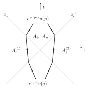
Fig. 1.: Domains of different time dependences. The fermion amplitude is a sum of two terms: one interacting first with the left moving nucleus, then the right moving one, and vice versa. $A_{i}^{(1,2)}$ are pure gauges and $A_{i},A_{\eta}$ is a numerically computed color field. In the perturbative limit of the Abelian theory these terms correspond to the $u$ and $t$ channel diagrams in Fig. 12.

2 The numerical calculation

Our calculation of pair production relies on the numerical calculation of the classical background color field, in which we solve the Dirac equation.

2.1 The background field

In the classical field model the background gluon field is obtained from solving the Yang-Mills equation of motion with the classical color source $J^{\nu}$ given by transverse color charge distributions of the two nuclei boosted to infinite energy:

$$[D_{\mu},F^{\mu\nu}]=J^{\nu}=\delta^{\nu+}\rho_{(1)}(\mathbf{x}_{T})\delta(x^{-})+\delta^{\nu-}\rho_{(2)}(\mathbf{x}_{T})\delta(x^{+}).$$ (1)

In the MV model [10] the color charges are taken to be random variables with a Gaussian distribution

$$\langle\rho^{a}(\mathbf{x}_{T})\rho^{b}(\mathbf{y}_{T})\rangle=g^{2}\mu^{2}\delta^{ab}\delta^{2}(\mathbf{x}_{T}-\mathbf{y}_{T})$$ (2)

depending on the coupling $g$ and a phenomenological parameter $\mu$. The combination $g^{2}\mu$ is closely related to the saturation scale $Q_{\mathrm{s}}$. Collisions of two ions were first studied analytically using this model in Ref. [11] and the way of numerically solving the equations of motion in a Hamiltonian formalism in the $A_{\tau}=0$ gauge was formulated in Ref. [12].

2.2 Solving the Dirac equation

Our method of solving the Dirac equation is explained in more detail and the numerics tested in a 1+1-dimensional toy model in Ref. [13]. The domains of spacetime involved in the calculation are illustrated in Fig. 1.

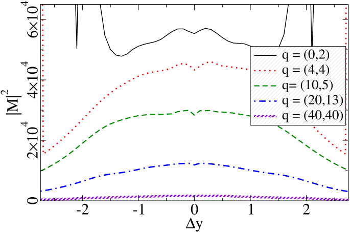
Fig. 2.: Amplitude (in lattice units) at $\tau=0.25\textrm{ fm}$ as a function of $\Delta y$ for different antiquark momenta on a $180^{2}$-lattice (see text in Sec. 2.4 for the notation).

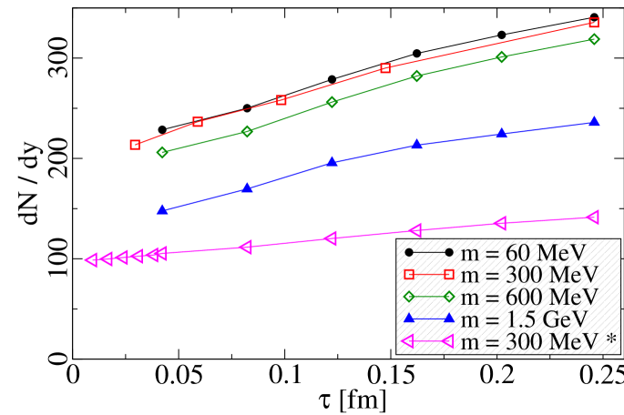
Fig. 3.: Dependence on proper time $\tau$ of the number of pairs of one flavor per unit rapidity $\mathrm{d}N/\mathrm{d}y$ for $g^{2}\mu=2$ GeV and different quark masses. The lowest curve corresponds to $g^{2}\mu=1\textrm{ GeV}$.

One starts in the the infinite past $t\to-\infty$ with a negative energy plane wave solution $\psi(x)=e^{iq\cdot x}v(q)$. The Dirac equation can then be integrated forward in time analytically to the future light cone ($\tau^{2}=2x^{+}x^{-}=0,\ x^{\pm}>0$) because the background field in the intermediate region is a pure gauge. This gives an initial condition, given explicitly in Eq. (16) of Ref. [13], for $\psi(\tau=0,z,\mathbf{x}_{T})$. Starting from this initial condition we then solve numerically the Dirac equation for $\tau\geq 0$ using the coordinate system $\tau,z,\mathbf{x}_{T}$. The reason for this choice of coordinates is the following. It not feasible to have degrees of freedom at different energy scales ($\sqrt{s}$ and $Q_{\mathrm{s}}$) present in the same numerical calculation. Thus the temporal coordinate is chosen to be $\tau$ in order to include the hard sources of the color fields only in the initial condition. Although the background field is boost invariant, the longitudinal coordinate can not be disregarded in this computation because the rapidities of the quark and the antiquark are correlated. The longitudinal coordinate is chosen as $z$, not the usual dimensionless $\eta=\tanh^{-1}(z/t)$, because the initial condition on the light cone involves dimensionful longitudinal momentum scales (coming from the four momentum $q$), and in order to represent them on a spatial lattice at $\tau=0$ a dimensionful coordinate is needed.

The pair production amplitude $M_{\tau}$ at proper time $\tau$ is then obtained by fixing the Coulomb gauge in the transverse plane $\partial_{i}A_{i}=0$ and projecting the spinor wavefunction $\psi(\tau,z,\mathbf{x}_{T})$ onto positive energy states $\phi_{p}(\tau,z,\mathbf{x}_{T})\equiv e^{-ip\cdot x}u(p)$:

$$M_{\tau}(p,q)\equiv\int\frac{\tau\mathrm{d}z\mathrm{d}^{2}\mathbf{x}_{T}}{\sqrt{\tau^{2}+z^{2}}}\,\phi_{p}^{\dagger}(\tau,z,\mathbf{x}_{T}){\gamma^{0}}\gamma^{\tau}\psi_{q}(\tau,z,\mathbf{x}_{T}).$$ (3)

For times larger than the formation time of the quark pair $\tau\gtrsim 1/\sqrt{m^{2}+{\mathbf{q}_{T}}^{2}}$ this amplitude can be interpreted as the amplitude for producing quark antiquark pairs.

2.3 Results

Figure 3 shows $|M_{\tau}|^{2}$ as a function of $\Delta y=y_{p}-y_{q}$ integrated over ${\mathbf{p}_{T}}$ for different ${\mathbf{q}_{T}}$. When integrating also over the rapidity difference $\Delta y$ one gets the number of pairs per unit rapidity as a function of $\tau$, shown in Fig. 3. It can be seen that the quark production amplitude reaches a finite value instantaneously and then increases slowly with $\tau$.

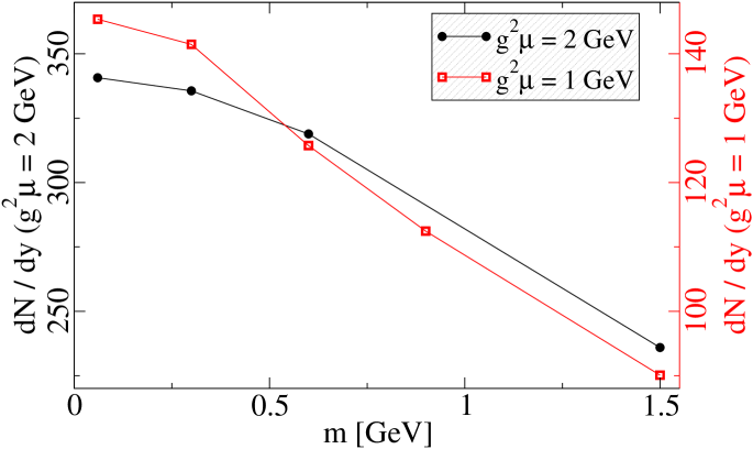
Fig. 4.: Dependence of the number of quark pairs on quark mass at a fixed proper time, $\tau=0.25\textrm{ fm}$, and for two values of $g^{2}\mu$.

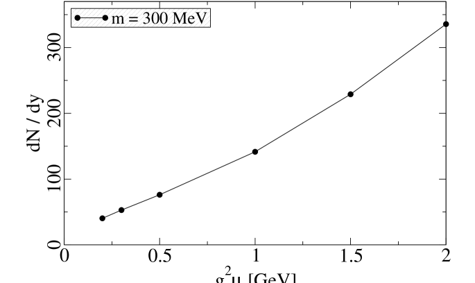
Fig. 5.: Dependence of the number of quark pairs on $g^{2}\mu$ at a fixed proper time, $\tau=0.25\textrm{ fm}$, and for quark mass $m=0.3\textrm{ GeV}$.

The physical parameters of the calculation are $g^{2}\mu$ characterizing the strength of the background field, the nuclear radius $R_{A}$ and the quark mass $m$. The dependence on $g^{2}\mu$ and $m$ of the number of pairs at $\tau=0.25\textrm{ fm}$ is shown in Figs. 5 and 5. The number of pairs is seen to increase with $g^{2}\mu$, but not as strongly as the $(g^{2}\mu)^{2}$ dependence predicted by a simple dimensional analysis argument. The result also decreases with increasing quark mass, but the perturbative $1/m^{2}$-behavior is not reached in our calculation. The transverse momentum spectra of the (anti)quarks as a function of ${\mathbf{q}_{T}}$ is shown for different quark masses and saturation scales in Figs. 7 and 7.

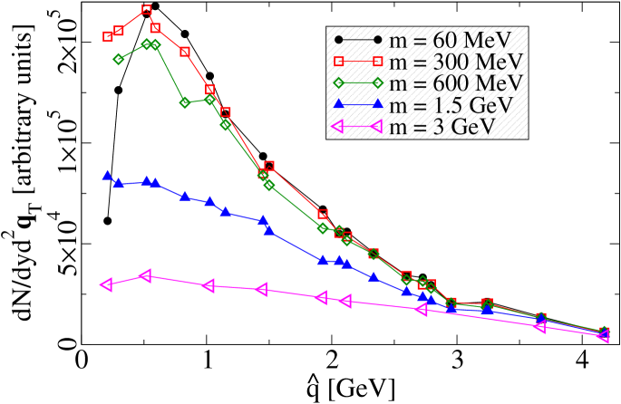
Fig. 6.: Transverse momentum spectrum of (anti)quarks for $g^{2}\mu=2$ GeV at a fixed proper time, $\tau=0.25$ fm, and for different quark masses.

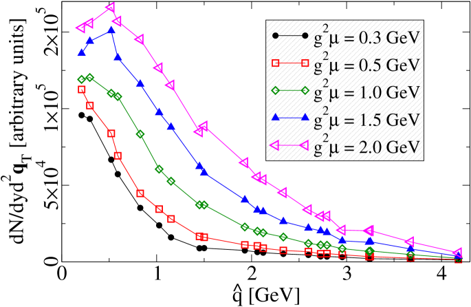
Fig. 7.: Transverse momentum spectrum of (anti)quarks for quark mass $m=0.3$ GeV and for different $g^{2}\mu$ at a fixed proper time, $\tau=0.25$ fm.

2.4 The numerical method

Our numerical method is presented in more detail in Refs. [13, 14]. The discretization in the transverse plane is straightforward, but in the longitudinal direction the $\tau,z$ coordinate system can easily result in an unstable one. In Ref. [13] a stable scheme was found by using an implicit method, where at each timestep one solves a linear system of equations for the spinor at different points on the longitudinal lattice.

The numerical computation depends on several discretization parameters: the lattice size and spacing in the longitudinal ($N_{z}$ and $\mathrm{d}z$) and the transverse ($N^{2}$ and $a$) directions and the timestep $\mathrm{d}\tau$. To check our numerical method we studied the dependence on these parameters. We have also tested the numerical method in the analytically solvable case of zero external field and tested how well our numerical implementation preserves boost invariance.

The dependence on the longitudinal lattice parameters, $\mathrm{d}z$ and $N_{z}$, is studied in Figs. 9 and 9. Our convention is that the longitudinal lattice has points $i=-N_{z}\dots N_{z}$, i.e. $2N_{z}+1$ points and the length of the longitudinal lattice is $2N_{z}\mathrm{d}z$. The results presented earlier in this talk are for $\mathrm{d}z=0.2a$ and $N_{z}=200$ and have not been extrapolated to the infinite volume limit $N_{z}\mathrm{d}z\to\infty$. A finite $\mathrm{d}z$ leads to a lattice cutoff in $p^{z}$ and thus sets a maximum for the accessible interval in $\Delta y$. As can be seen from Fig. 3 and understood as a consequence of the initial condition, Eq. (16) of Ref. [13], the accessible region in $\Delta y$ is smaller for small transverse momenta ${\mathbf{q}_{T}}$. This cutoff in $\Delta y$ is also apparent in Figs. 9, 11 and 11.

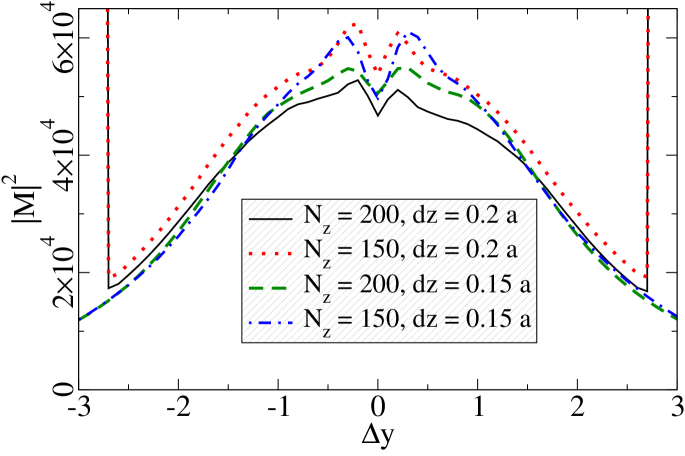
Fig. 8.: Amplitude at $\tau=0.25\textrm{ fm}$ for $g^{2}\mu=2\textrm{ GeV}$ for different values of $\mathrm{d}z$ and $N_{z}$ . The lattice spacing is measured in units of $a$, the transverse lattice spacing.

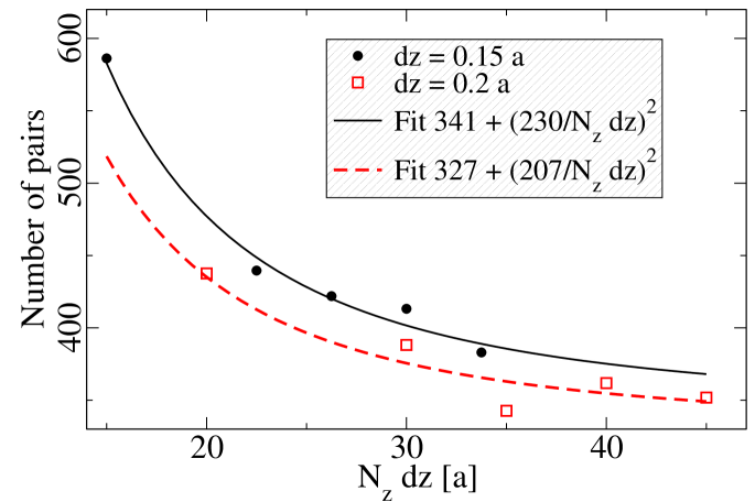
Fig. 9.: Number of pairs as a function of (half) the volume of the longitudinal lattice $N_{x}\mathrm{d}z$ for two different values of $\mathrm{d}z$. The solid lines are fits of the form $A+B/(N_{z}\mathrm{d}z)^{2}$.

We have so far only used transverse lattices of $180^{2}$ points. The lattice momenta can be represented as ${\mathbf{q}_{T}}=(q_{x},q_{y})$ with $q_{x,y}=-89\dots 90$, of which the $q_{x,y}=-45\dots 45$ are non-doubler modes. We explicitly leave out the doubler modes both in the initial condition (${\mathbf{q}_{T}}$ modes) and in the projection to the positive energy state (${\mathbf{p}_{T}}$ modes). This limits the volume of the transverse momentum space to $1/4$ of the bosonic case. Also the spectrum of quarks (see Figs. 7 and 7) decreases so slowly for large transverse momenta that some dependence on the $1/a$ lattice cutoff is expected. Further computations with larger transverse lattices are still needed to study this issue.

The memory requirement for a $400\times 180^{2}$–lattice with $4\times(N_{\mathrm{c}}=3)$ complex components in one spinor is $1.2\textrm{ GB}$ in single precision. This can still be achieved on one processor, but for larger lattices a parallelized version of the program will have to be used. The numerical computations have been done on the “ametisti” cluster, a $66\times 2$ processor AMD Opteron Linux cluster at the University of Helsinki, using over $10^{17}$ flop of CPU-time so far.

As explained in Fig. 1, the amplitude is a sum of two terms. For a zero external color field these two terms, with an absolute value $|M_{\tau}|=1/\cosh(\Delta y/2)$ have an opposite sign and cancel each other. Comparing the analytically and numerically computed amplitudes is a nontrivial test of the numerical computation. Figure 11 shows how the analytical result for one branch and the cancellation when both branches are included are reproduced by our numerical method for one value of ${\mathbf{q}_{T}}$ (${\mathbf{q}_{T}}=(5,5)$ on a $150^{2}$ lattice).

Due to the boost invariance of the background field the amplitude $M_{\tau}$ should not depend on the rapidities $y_{q}$ and $y_{p}$ separately, but only on the difference $\Delta y\equiv y_{p}-y_{q}$. Because the calculation is done using $z$, not rapidity, as the longitudinal coordinate, verifying the boost invariance of the resulting amplitude is a nontrivial test of the numerical method. Figure 11 shows that the number of pairs is, taking into account numerical inaccuracies, not affected by the choice of $y_{q}$.

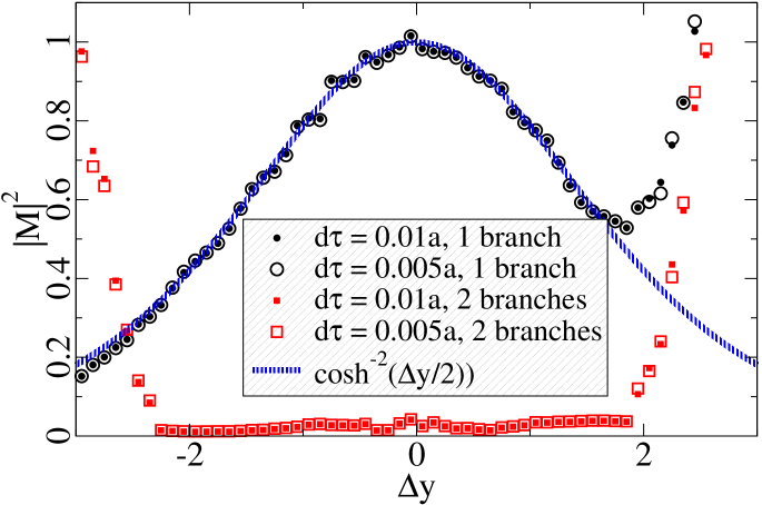
Fig. 10.: The amplitude in a zero external color field for two different timesteps $\mathrm{d}\tau$. Plotted are the absolute value of the amplitude for only one and both branches of the amplitude (see text and Fig. 1).

Fig. 11.: The amplitude $|M_{\tau}|^{2}$ as a function of the rapidity difference $\Delta y$ for different rapidities of the antiquark $y_{q}$.

3 Discussion

It has conventionally been assumed that the initial state of a heavy ion collision is dominated by gluons. This is the result e.g. when both quarks and gluons are produced in $2\to 2$ collisions of collinear partons [15]. Indeed, when comparing the cross sections of the $2\to 2$ processes for quark pair production and gluon production (see Fig. 12), the diagrams for quark pair production are suppressed by a factor of $\sim 210=7\times 30$, of which the factor 7 is due to color factors.

In the color glass condensate framework the picture is quite different. Whereas the quark pairs are produced in a $2\to 2$ process similarly to collinear factorisation, gluons are produced in what reduces in the perturbative limit to a $2\to 1$ process with a smaller power of the coupling $g$. It is therefore less straightforward to compare the two. Strictly perturbatively quark pair production is of higher order in $g$. But the phenomenologically relevant value is $g\approx 2$, and thus higher orders in $g$ are not suppressed by much when looking at the actual numbers. One can then legitimately ask whether one should, for consistency, also include quantum corrections (higher orders in $g$) in the computation of gluon production.

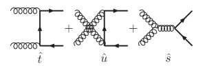
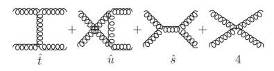
Fig. 12.: The 2 $\to$ 2-processes for producing quark pairs and gluons from an initial gluon distribution.

Brushing aside these remarks and boldly taking our numerical results at their face value would lead to the following scenario. It was earlier assumed that the initial state of a heavy ion collision is dominated by gluons. If the subsequent evolution of the system conserves entropy and thus, approximately, multiplicity this would mean $\sim 1000$ gluons in a unit of rapidity. In the classical field model this corresponds [16] to $g^{2}\mu\approx 2\textrm{ GeV}$. Our results seems to point to a rather large number of quark pairs present already in the initial state. One could envisage a scenario where for $g^{2}\mu\approx 1.3\textrm{ GeV}$ these 1000 particles could consist of $\gtrsim 400$ gluons, $\gtrsim 300$ quarks and $\gtrsim 300$ antiquarks (take the lowest curve from Fig. 3 and multiply by $N_{\mathrm{f}}=3$). This would be close to the thermal ratio of $N_{g}/N_{q}=64/(21N_{\mathrm{f}})$.

4 Conclusions

We have calculated quark pair production from classical background field of McLerran-Venugopalan model by solving the 3+1–dimensional Dirac equation numerically in this classical background field. We find that number of quarks produced is large, pointing to a possible fast chemical equilibration of the system. The mass dependence of our result surprisingly weak and we are not yet able to make any conclusions on heavy quarks until studying the numerical issues involved.

Acknowledgements

T.L. was supported by the Finnish Cultural Foundation. This research has also been supported by the Academy of Finland, contract 77744. We thank R. Venugopalan, H. Fujii, K. J. Eskola, B. Mueller and D. Kharzeev for discussions.

References

- [1] F. Gelis, K. Kajantie and T. Lappi, hep-ph/0508229.
- [2] F. Gelis, K. Kajantie and T. Lappi, hep-ph/0509343.
- [3] F. Gelis and R. Venugopalan, Phys. Rev. D69 (2004) 014019 [hep-ph/0310090].
- [4] H. Fujii, F. Gelis and R. Venugopalan, hep-ph/0504047.
- [5] A. J. Baltz and L. D. McLerran, Phys. Rev. C58 (1998) 1679 [nucl-th/9804042].
- [6] A. J. Baltz, F. Gelis, L. D. McLerran and A. Peshier, Nucl. Phys. A695 (2001) 395 [nucl-th/0101024].
- [7] D. Kharzeev and K. Tuchin, Nucl. Phys. A735 (2004) 248 [hep-ph/0310358].
- [8] K. Tuchin, Phys. Lett. B593 (2004) 66 [hep-ph/0401022].
- [9] D. D. Dietrich, Phys. Rev. D70 (2004) 105009 [hep-th/0402026].
- [10] L. D. McLerran and R. Venugopalan, Phys. Rev. D49 (1994) 2233 [hep-ph/9309289].
- [11] A. Kovner, L. D. McLerran and H. Weigert, Phys. Rev. D52 (1995) 3809 [hep-ph/9505320].
- [12] A. Krasnitz and R. Venugopalan, Nucl. Phys. B557 (1999) 237 [hep-ph/9809433].
- [13] F. Gelis, K. Kajantie and T. Lappi, Phys. Rev. C71 (2005) 024904 [hep-ph/0409058].
- [14] T. Lappi, hep-ph/0505095.
- [15] K. J. Eskola, K. Kajantie, P. V. Ruuskanen and K. Tuominen, Nucl. Phys. B570 (2000) 379 [hep-ph/9909456].
- [16] T. Lappi, Phys. Rev. C67 (2003) 054903 [hep-ph/0303076].