Inclusive spectra in charmless semileptonic B decays by Dressed Gluon Exponentiation

Abstract:

The triple differential spectrum in $\bar{B}\longrightarrow X_{u}l\bar{\nu}$ is computed by Dressed Gluon Exponentiation (DGE). In this framework the on-shell calculation, converted into hadronic variables, can be directly used as an approximation to the meson decay spectrum, without involving a leading–power non-perturbative function. Sudakov resummation for the fully differential $\bar{B}\longrightarrow X_{u}l\bar{\nu}$ width is formulated in moment space, where moments are defined using the ratio between the lightcone momentum components of the partonic jet $p^{+}/p^{-}$ and the hard scale is $p^{-}$. In these variables the correspondence with the $\bar{B}\longrightarrow X_{s}\gamma$ case is transparent. The Sudakov exponent is known to next–to–next–to–leading logarithmic accuracy. Further constraints are put on its Borel sum using the cancellation of the leading renormalon ambiguity and the absence of the next–to–leading one, which was proven in the large–$\beta_{0}$ limit and assumed here to be general. Based on the resummed spectrum, matched to the fully differential NLO result, we calculate the event fraction associated with experimental cuts on the hadronic mass (or the small lightcone component) as well as on the lepton energy. Finally, we extract $|V_{ub}|$ from recent measurements by Belle and analyze the theoretical uncertainty.

1 Introduction

A central issue on the agenda of the B factories is the precise determination of the CKM matrix element $V_{ub}$. Without undermining the significance of exclusive hadronic final–state analysis, measurements of the inclusive branching fraction of charmless semileptonic decays, $\bar{B}\longrightarrow X_{u}l\bar{\nu}$, provide the safest and most accurate determination of $\left|V_{ub}\right|$  [1, 2, 3, 4, 5, 6, 7].

Theoretically, because of the inclusive nature of the measurement, the calculation of the width $\Gamma\left(\bar{B}\longrightarrow X_{u}l\bar{\nu}\right)$ in units of $\left|V_{ub}\right|^{2}$ relies primarily on QCD perturbation theory. The final state, which in reality is composed of light hadrons, can be safely described in the course of the calculation by light quarks and gluons. Moreover, the dependence of the width on the internal dynamics of the decaying B meson is power suppressed. The Operator Product Expansion (OPE) implies that the total decay width of a B meson is equal to the total decay width of a hypothetical on-shell b quark up to ${\cal O}(\Lambda^{2}/m_{b}^{2})$ corrections, which can be expressed as forward matrix elements of certain local operators whose numerical values are determined based on other measurements. These corrections are very small.

The main obstacle in extracting $\left|V_{ub}\right|$ from inclusive semileptonic decays is the need to eliminate the huge background due to B decay into charm. The most effective way to maximize the rate while discriminating the charm background is to select events where the hadronic system has small mass, $M_{X}\mathrel{\mathchoice{\vbox{\offinterlineskip\halign{$\m@th\displaystyle\hfil#\hfil$\cr<\crcr\sim\crcr} }}{\vbox{\offinterlineskip\halign{$\m@th\textstyle\hfil#\hfil$\cr<\crcr\sim\crcr} }}{\vbox{\offinterlineskip\halign{$\m@th\scriptstyle\hfil#\hfil$\cr<\crcr\sim\crcr} }}{\vbox{\offinterlineskip\halign{$\m@th\scriptscriptstyle\hfil#\hfil$\cr<\crcr\sim\crcr} }}}1.7$ GeV, see e.g. [8, 9, 5, 7].

Because of the cuts, detailed theoretical understanding of the differential distribution is essential. In the small–$M_{X}$ region the hadronic system is most likely jet-like. Working with lightcone coordinates, $P^{+}\leq P^{-}\leq M_{B}$ with $M_{X}^{2}=P^{+}P^{-}$, the small $M_{X}$ region directly corresponds to the region where the smaller lighcone component gets small, $P^{+}\longrightarrow 0$, so it involves highly non-local correlation functions with large lightcone separation, $y^{-}\longrightarrow\infty$, where $y^{-}$ is the Fourier conjugate to $P^{+}$. At leading power in ${\cal O}(\Lambda/m_{b})$ the differential width involves the full lightcone momentum distribution function of the b quark inside the meson, the so-called “shape function” [10, 11]. On the non-perturbative level, not much is known about this distribution: it is difficult to compute it on the lattice and although in principle it can be measured using the photon spectrum in rare radiative decays $\bar{B}\longrightarrow X_{s}\gamma$, realistic measurements constrain just the first few moments of this function [12, 13].

As it stands, the theoretical uncertainty in extracting $\left|V_{ub}\right|$ from inclusive semileptonic decays is dominated by the uncertainty in estimating the effect of cuts. A great variety of experimental cuts has been proposed, which either aim at reducing the sensitivity to the unknown momentum distribution of the b quark in the meson by cutting out the phase–space regions where it is important [14, 15], or alternatively, aim at making the relation with the $\bar{B}\longrightarrow X_{s}\gamma$ spectrum as direct as possible [16, 18, 17, 19]. While the comparison between results for $\left|V_{ub}\right|$ obtained using different cuts is useful for controlling experimental as well as theoretical uncertainties, better measurements can be achieved if cuts would be chosen based on purely experimental considerations. Precise theoretical predictions for the fully differential width are therefore urgently needed.

1.1 The applicability of perturbation theory

In perturbation theory, the fully differential width is currently known [20] to the next–to–leading order (NLO), which includes tree level as well as one–loop, i.e. ${\cal O}(\alpha_{s})$, virtual corrections, where the hadronic system is represented by a single on-shell $u$ quark, as well as bremsstrahlung contributions where the hadronic system is composed of a u-quark and a gluon, and therefore has a non-vanishing mass. It has long been recognized that fixed–order calculations do not provide even a qualitative description of the differential width in the small–$M_{X}$ region, where multiple emission of soft and collinear gluons is important [21, 24, 25, 30, 31, 23, 22, 26, 27, 28, 29]. In terms of partonic lightcone coordinates, $p_{j}^{+}\leq p_{j}^{-}\leq m_{b}$, the small $M_{X}$ region is characterized by a large hierarchy, $p_{j}^{+}/p_{j}^{-}\ll 1$. Higher–order corrections containing Sudakov logarithms of the ratio $p_{j}^{+}/p_{j}^{-}$ are large, and they must be resummed to all orders to recover the characteristic Sudakov peak at small $M_{X}$.

According to the factorization properties of the fully differential width in inclusive decays [21, 24, 25, 30, 31, 23, 22, 26, 27, 28, 29], Sudakov logarithms exponentiate in moment space. We shall work here with moments $n$ defined with respect to powers of $1-p_{j}^{+}/p_{j}^{-}$, as in Eq. (3.2) below. The region of interest, of small $p_{j}^{+}$, is probed by high moments, $n\longrightarrow\infty$. The logarithms, $\ln n$, which become large in this limit, originate in two distinct subprocesses of different characteristic scales, which factorize in this moment space. The first is the final–state jet having a constrained invariant mass squared of ${\cal O}(m_{b}^{2}/n)$ [32, 30, 31], which coincides with the Sudakov factor of deep inelastic structure functions. The second corresponds to the quark distribution in an on-shell heavy quark, the perturbative analogue of the quark distribution in the meson [30, 33, 31], and describes soft radiation, $|k|\sim{\cal O}(m_{b}/n)$, from the nearly on-shell heavy quark prior to the decay.

A major stumbling block, which essentially prohibits the straightforward application of Sudakov resummation to inclusive B decay phenomenology, is that the scales involved are almost too low for perturbation theory to apply. While the b quark mass is heavy compared to the QCD scale $\Lambda$, in the Sudakov limit, $n\longrightarrow\infty$, the jet mass scale is much lower than $m_{b}$ and the soft scale $|k|\sim{\cal O}(m_{b}/n)$ characterizing the quark distribution is yet much lower. Already at moderately high moments, $n\sim 10$, the latter is dangerously close to $\Lambda$ where the physics in non-perturbative. On these grounds it is often argued [34, 35] that Sudakov resummation is useless in this case. Conversely, when Sudakov resummation is applied it is usually supplemented by an external infrared cutoff along with parametrization of the non-perturbative quark distribution function below this scale [16, 17].

While there are many ways to partially bypass the need to resum corrections on the scale $|k|\sim{\cal O}(m_{b}/n)$, we argue that this resummation is in fact largely under control and that it is very useful. Ref. [31] and the present investigation show that definite predictions emerge when the available information on the large–order behavior of the perturbative expansion is taken into account. The sensitivity to low momentum scales, and specifically to the meson structure, turns out to be smaller than it superficially appears to be, and consequently the predictive power of perturbation theory is higher than what one might a priori expect.

Infrared sensitivity appears in the moment–space Sudakov exponent through infrared renormalons [36, 32, 39, 37, 38, 40, 41, 33]. These generate divergences and invalidate the logarithmic accuracy criterion [30, 31], but they definitely do not prohibit using Sudakov resummation altogether: the Sudakov exponent needs to be regarded as an asymptotic series, and summed up to all orders by regularizing the renormalons in a systematic way. This is the essence of Dressed Gluon Exponentiation (DGE). The application of this approach to inclusive decays is particularly advantageous since the leading infrared renormalon ambiguity, which dictates the divergence of the series in the Sudakov exponent, cancels exactly with the pole–mass ambiguity that is carried by kinematic power corrections associated with the conversion from partonic to hadronic variables. In this way, the on-shell calculation becomes directly useful for phenomenology, in spite of the divergence of the series (or the ambiguity) that appeared at the intermediate stage.

In the present paper we provide precise theoretical predictions for the fully differential width in semileptonic decays using DGE. Our calculation makes maximal use of Sudakov resummation and the underlying renormalon structure. In this way we effectively minimize the role of the unknown non-perturbative component of the quark–distribution function and the associated uncertainties.

The method of DGE was already proven successful in the application to the photon energy spectrum in $\bar{B}\longrightarrow X_{s}\gamma$ decays [31, 41]. Specifically, the first two central moments defined over the range $E_{\gamma}>E_{0}$, were computed in [31] in an essentially perturbative fashion (see below) without involving any parametrization of the leading–power quark distribution function. These predictions were later compared [41] with experimental measurements from Babar [42] over a wide range of cuts, $E_{0}=1.9$ to 2.26 GeV, finding very good agreement.

1.2 Comparison with alternative approaches

It is worthwhile re-examining from the present perspective the conventional approach to inclusive spectra, which is based on parametrizing the leading–power non-perturbative “shape function” [10, 11] in analogy with deep inelastic structure–function phenomenology. Let us summarize the qualitative differences.

In Refs. [10, 11, 17] one begins by considering directly the kinematic region where the small lightcone component of the hadronic system is comparable to the momentum of the light degrees of freedom in the meson, ${\cal O}(\Lambda)$. In the $m_{b}\longrightarrow\infty$ limit the long–distance interaction is captured by a single lightcone distribution, the “shape function”. No attempt is made to compute this function, which is assumed non-perturbative from the beginning. The “shape function” is parametrized and the parameters are fixed by a fit to the measured $\bar{B}\longrightarrow X_{s}\gamma$ spectrum (see e.g. Sec. 4 in Ref. [17]). Owing to the universality of this function, the result can be directly used in semi-leptonic decays. There is of course some bias owing to the functional form assumed. In practice this can be dealt with by varying the function, or better, by relating directly the semileptonic distribution to the $\bar{B}\longrightarrow X_{s}\gamma$ data by weighted integrals [18, 19].

Our approach is more ambitious: we wish to compute the spectrum. Relying on the fact that the heavy quark in the meson is rarely far off shell, we compute the on-shell decay spectrum and use it as a first approximation to the meson decay spectrum. In this approximation the quark distribution in the meson is replaced by its perturbative analogue, the quark distribution in an on-shell heavy quark — see Ref. [33] for the precise definition. A key element in this approach is the systematic treatment of infrared renormalons. Most importantly, this includes a systematic definition of the on-shell heavy quark state at the level of resummed perturbation theory. Having full control of the large–order behavior of the expansion, such definition is provided by Principal Value Borel summation. Upon consistently using this definition in both the Sudakov exponent and the quark pole mass (which enters the computed spectrum through the conversion to hadronic variables) any ${\cal O}(\Lambda/m_{b})$ ambiguities are avoided. In this way resummed perturbation theory yields definite predictions for the on-shell decay spectrum. The latter provides an approximation to the meson decay spectrum that does not require any ${\cal O}(\Lambda/m_{b})$ non-perturbative power corrections. Having established that, we study higher power corrections that constitute the ratio between the moments of the physical spectrum and the computed one, which originate in the dynamical structure of the meson. While these corrections gradually increase with the moment index $n$ they have but a small effect on the global properties of the spectrum.

It should be emphasized that in reality the spectrum in the immediate vicinity of the endpoint, $P^{+}\simeq 0$, cannot be accurately described by any of these approaches for two reasons: first, the number of relevant “shape function” parameters increases, and second, the transition to the exclusive region, namely the hadronic structure of the final state, is not addressed.

Recent formulations of the “shape function” approach, e.g. [17], employ the tools of factorization [21, 22] and can therefore make some use of Sudakov resummation. Nevertheless the resummation there effectively concerns the jet function only, as the “shape function” is defined at an intermediate scale of order of the jet mass. Moreover, the need to separate “jet” logarithms from “soft” ones requires a complicated infrared cutoff to be introduced at any order in perturbation theory. The final answer is affected by residual scale and scheme dependence.

In contrast, in our formulation Sudakov resummation is applied also to the quark–distribution function. We thus make full use of the available perturbative information. Moreover, the on-shell decay spectrum we compute is itself renormalization group invariant: it is absolutely free of any factorization scale or scheme dependence; at the level of the Sudakov factor, it is also free of renormalization–scale dependence owing to the additional resummation of running–coupling effects we perform.

The conclusion from Ref. [31] and the successful comparison with experimental data [41] is that when using DGE, the on-shell calculation, $b\longrightarrow X_{s}\gamma$, converted into hadronic variables, directly provides a good approximation of the B meson decay spectrum. Notably, in contrast with any fixed–order approximation, it has approximately correct physical support properties at large $E_{\gamma}$. This implies, in particular, that in this framework the non-perturbative component of the lightcone momentum distribution function is small, and at the present accuracy can even be neglected. This conclusion may be surprising: as discussed above, in other approaches the parametrization of this non-perturbative distribution is absolutely essential. In order to understand the difference one should recall that

(1)  The separation between the perturbative and non-perturbative components of the lightcone momentum distribution function depends on the convention adopted. In our approach, the calculated perturbative component is nothing but the quark distribution in an on-shell heavy quark. It requires renormalization owing to logarithmic ultraviolet singularities, however, no infrared cutoff is needed. This distribution is infrared and collinear safe and therefore well–defined to all orders in perturbation theory. It requires of course Sudakov resummation, owing to the large hierarchy between the hard scale $m_{b}$ and the soft scale $m_{b}/n$. In contrast, at the power level the Sudakov exponent is infrared sensitive: its Borel sum has ambiguities scaling as powers of $(n\Lambda/m_{b})$. In our approach these are regularized using the Principal Value prescription — this is how we define the perturbative component of the quark distribution function.

(2)  Beyond the currently available logarithmic accuracy at which the quark distribution is known (next–to–next–to–leading logarithmic accuracy [33]), the DGE calculation makes use of additional information, which is important in constraining the corresponding Borel sum. Most importantly, the exact cancellation of the leading ($u=1/2$) renormalon ambiguity with kinematic power corrections involving the pole mass [30] is used to fix the corresponding residue [31]. In addition, the absence of the next–to–leading renormalon ($u=1$), which was proven in the large–$\beta_{0}$ limit [30], is assumed here to be general. Thus, the dependence on the (Principal Value) prescription is eventually restricted to higher renormalons ($u\geq 3/2$), which have limited influence on the spectrum — see Ref. [31] and below.

Following the results of Refs. [31, 41], our working assumption in this paper is that the properly–defined quark distribution in an on-shell heavy quark provides a good approximation to the quark distribution in the meson. In reality the two differ of course, and it is important to quantify the power corrections that distinguish between them, a task that will require theoretical as well as experimental input. This, however, is beyond the scope of the present paper.

1.3 The task and the strategy

The main task on which we embark here is to provide a reliable calculation of the partial decay width with experimentally–driven cuts. Priority is given to cuts that maximize the rate, in particular [7] the charm–discriminating cut on the hadronic mass $P^{+}P^{-}<M_{X}^{2}=(1.7\,{\rm GeV})^{2}$ with an additional, experimentally unavoidable, mild cut on the charged lepton energy $E_{l}>1$ GeV. Our general strategy to extract $\left|V_{ub}\right|$ from data is based on separately computing:

• The total charmless semileptonic width $\Gamma_{\hbox{\tiny total}}\left(\bar{B}\longrightarrow X_{u}l\bar{\nu}\right)$ in units of $\left|V_{ub}\right|^{2}$, using the available NNLO result [43] and renormalon resummation.

• The effect of experimental cuts as the event fraction

  $$R_{\rm cut}\equiv\frac{\Gamma(\bar{B}\longrightarrow X_{u}l\bar{\nu}\,\,{\rm restricted\,\,phase\,\,space})}{\Gamma(\bar{B}\longrightarrow X_{u}l\bar{\nu}\,\,{\rm entire\,\,phase\,\,space})},$$ (1)

  which we compute using DGE and match to the fully differential NLO result in moment space.

The partial branching ratio measured by the B factories can then be compared to

$$\Delta{\cal B}(\bar{B}\longrightarrow X_{u}l\bar{\nu}\,\,{\rm restricted\,\,phase\,\,space})=\tau_{B}\Gamma_{\hbox{\tiny total}}\left(\bar{B}\longrightarrow X_{u}l\bar{\nu}\right)R_{\rm cut}.$$ (2)

The advantages in splitting the calculation of the partial width this way are:

• The event fraction $R_{\rm cut}$ is free of the ${\cal O}(\Lambda/m_{b})$ renormalon ambiguity associated with the overall factor $m_{b}^{5}$ where $m_{b}$ is the quark pole mass. Note that ${\cal O}(n\Lambda/m_{b})$ cut–related renormalon ambiguities are present in the perturbative result for $R_{\rm cut}$, but their effect is restricted to the moment–space Sudakov exponent. Therefore, the perturbative expansion of the hard matching coefficient for $R_{\rm cut}$ is renormalon free and truly dominated by hard scales at higher orders.

• The total charmless semileptonic width can be computed with NNLO accuracy and in a way that renormalon–related ${\cal O}(\Lambda/m_{b})$ power effects explicitly cancel. One then obtains the total width with theoretical uncertainty as low as $\sim 6\%$. Such accuracy cannot be achieved in a direct calculation of the partial width in the restricted phase–space since (1) the differential width is known in full only to NLO accuracy; and (2) while Sudakov resummation can be used to take into account parametrically–enhanced corrections associated with the phase-space restriction, some residual uncertainty of both perturbative and non-perturbative nature remains. Quantitative estimates are provided in Sec. 4.2.

The paper is divided into three main sections. In Sec. 2 we compute the total semileptonic width using the NNLO result [43] and renormalon resummation. In Sec. 3 we present the results for resummation of the triple–differential width and work out NLO matching formulae in moment space. Finally, in Sec. 4 we use these results to compute the differential and partially–integrated width in hadronic variables, taking into account the mass difference between the B meson and the b quark. In this section we study the theoretical uncertainty in $R_{\rm cut}$ and extract $\left|V_{ub}\right|$ from recent measurements by Belle [7].

2 The total charmless semileptonic decay width

According to the OPE the total $\bar{B}\longrightarrow X_{u}l\bar{\nu}$ decay width is given by

$$\Gamma_{\hbox{\tiny total}}\left(\bar{B}\longrightarrow X_{u}l\bar{\nu}\right) = \frac{G_{F}^{2}\left|V_{ub}\right|^{2}m_{b}^{5}}{192\pi^{3}}F(\alpha_{s}(m_{b}))$$

$$= \frac{G_{F}^{2}\left|V_{ub}\right|^{2}m_{b}^{5}}{192\pi^{3}}\left[1+a_{0}\frac{\alpha_{s}(m_{b})}{\pi}+a_{1}\left(\frac{\alpha_{s}(m_{b})}{\pi}\right)^{2}+\cdots\,+\,{\cal O}\left(\frac{\Lambda^{2}}{m_{b}^{2}}\right)\right],$$

where the perturbative expansion has been computed to NNLO [43] and the matrix elements controlling the ${\cal O}\left({\Lambda^{2}}/{m_{b}^{2}}\right)$ terms are not large and amount to $\sim 1\%$ correction.

It is well known [44, 46, 45] that while the decay width receives just small ${\cal O}(\Lambda^{2}/m_{b}^{2})$ power corrections, the perturbative expansions of (a) the ratio between the pole mass and short–distance masses (e.g. $m_{b}^{\hbox{\tiny${\overline{\rm MS}}$}}$); and (b) the function $F(\alpha_{s}(m_{b}))$ in Eq. (2) have large ${\cal O}(\Lambda/m_{b})$ renormalon ambiguities owing to infrared sensitivity. Furthermore, the first few terms in these expansions show poor convergence; the asymptotic behavior sets in early. A practical problem one needs to address is how to optimally use the known coefficients in these expansions to get a reliable estimate of $\Gamma_{\hbox{\tiny total}}$ in Eq. (2). Often (e.g. [17, 34]) this problem is solved by resorting to a specific mass scheme where the mass and the perturbative expansion of the width are separately renormalon free, and hopefully converge well. Our approach is different. We use the pole mass itself and regularize the leading renormalon using Borel summation, explicitly using the cancellation in Eq. (2).

In Ref. [31] we studied the mass ratio and expressed it as a Borel integral where the Borel function is written as a bi-local expansion [49, 50, 48]

$$\frac{m_{b}}{m_{b}^{\hbox{\tiny${\overline{\rm MS}}$}}}\,=\,1+\frac{C_{F}}{\beta_{0}}\int_{0}^{\infty}dz\sum_{i=0}^{i_{\max}}b_{i}\,z^{i}+\frac{q}{(1-2z)^{1+\frac{1}{2}\delta}}\left[1+\sum_{k=1}^{k_{\max}}c_{k}(1-2z)^{k}\right],$$ (4)

where $\delta\equiv\beta_{1}/\beta_{0}^{2}$, $c_{k}$ depend on the coefficients of the $\beta$ function (see Appendix B in [31]), and the coefficients $b_{i}$ in the regular part of the expansion can be determined through order $b_{2}$ knowing the N³LO result [51] for the mass ratio. Here both the exact analytic structure of the singularity [52] and the value of the residue $q$ fixing the large–order asymptotic behavior of the expansion are used. The latter can be determined with $\mathrel{\mathchoice{\vbox{\offinterlineskip\halign{$\m@th\displaystyle\hfil#\hfil$\cr<\crcr\sim\crcr} }}{\vbox{\offinterlineskip\halign{$\m@th\textstyle\hfil#\hfil$\cr<\crcr\sim\crcr} }}{\vbox{\offinterlineskip\halign{$\m@th\scriptstyle\hfil#\hfil$\cr<\crcr\sim\crcr} }}{\vbox{\offinterlineskip\halign{$\m@th\scriptscriptstyle\hfil#\hfil$\cr<\crcr\sim\crcr} }}}3\%$ accuracy [50, 53, 54, 31] using the N³LO result for the mass ratio. Hence, given a definite integration prescription in the complex $z$ plain to avoid the $z=\frac{1}{2}$ singularity, Eq. (4) facilitates an accurate calculation of both the ${\cal O}(1)$ real and the ${\cal O}(\Lambda/m_{b})$ imaginary parts of the mass ratio. With the central values of the residue from Ref. [31],

$$C_{F}q(N_{f}=3)/\pi=0.560;\qquad C_{F}q(N_{f}=4)/\pi=0.536,$$ (5)

one obtains:

$$\left.\frac{m_{b}}{m_{b}^{\hbox{\tiny${\overline{\rm MS}}$}}}\right|_{N_{f}=3}\,=\,1.161\,-\,0.0934\,i\;\qquad\left.\frac{m_{b}}{m_{b}^{\hbox{\tiny${\overline{\rm MS}}$}}}\right|_{N_{f}=4}\,=\,1.164\,-\,0.0768\,i,$$ (6)

respectively. The variation in the number of light fermions is used to estimate charm mass effects. Here we chose to define the Borel sum in Eq. (4) with the integration contour going below the real axis avoiding the singularity at $z=\frac{1}{2}$. This fixes the imaginary part of the mass ratio (the physical real part is prescription independent). We evaluated the integrals using:

$$\int_{0}^{\infty}dz\frac{{\rm e}^{-z/A}}{\left(1-\frac{z}{z_{0}}\right)^{1+\nu}} = \frac{A}{\Gamma(1+\nu)}\int_{0}^{\infty}dl\frac{{\rm e}^{-l}l^{\nu}}{1-\frac{lA}{z_{0}}}=\frac{z_{0}}{\Gamma(1+\nu)}\frac{\pi}{\sin(\pi\nu)}\,{\rm e}^{-z_{0}/A}(-z_{0}/A)^{\nu}$$ (7)

$$+A^{1-\frac{1}{2}\nu}z_{0}^{\frac{1}{2}\nu}\frac{{\rm e}^{-\frac{1}{2}z_{0}/A}}{1-\nu}\bigg{[}M_{\frac{1}{2}\nu,\frac{1}{2}-\frac{1}{2}\nu}\left(z_{0}/A\right)-\frac{1}{\nu}M_{1+\frac{1}{2}\nu,\frac{1}{2}-\frac{1}{2}\nu}\left(z_{0}/A\right)\bigg{]},$$

where we assumed that $z_{0}=\frac{1}{2}+i\varepsilon$ where $\varepsilon$ is an infinitesimally small positive number, and $M_{\mu,\nu}(a)$ is the Whittaker $M$ function,

$$M_{\mu,\nu}(a)={\rm e}^{-\frac{1}{2}a}a^{\frac{1}{2}+\nu}\,_{1}F_{1}\left(\Big{[}\frac{1}{2}+\nu-\mu\Big{]},\Big{[}1+2\nu\Big{]},a\right).$$

The next crucial observation is that the cancellation of the leading renormalon ambiguity in Eq. (2) implies that

$$\frac{{\rm Im}\left\{F^{1/5}(\alpha_{s}(m_{b}))\right\}}{{\rm Re}\left\{F^{1/5}(\alpha_{s}(m_{b}))\right\}}=-\frac{{\rm Im}\left\{\frac{m_{b}}{m_{b}^{\hbox{\tiny${\overline{\rm MS}}$}}}\right\}}{{\rm Re}\left\{\frac{m_{b}}{m_{b}^{\hbox{\tiny${\overline{\rm MS}}$}}}\right\}}\,=\,{\cal O}(\Lambda/m_{b}),$$ (8)

and that the observable itself can be computed with ${\cal O}(\Lambda^{2}/m_{b}^{2})$ accuracy using the real parts (or Principal Value) of the mass ratio and $F^{1/5}$:

$$m_{b}F^{1/5}(\alpha_{s}(m_{b}))=m_{b}^{\hbox{\tiny${\overline{\rm MS}}$}}\times{\rm Re}\left\{\frac{m_{b}}{m_{b}^{\hbox{\tiny${\overline{\rm MS}}$}}}\right\}\times{\rm Re}\left\{F^{1/5}(\alpha_{s}(m_{b}))\right\}.$$ (9)

Eq. (8) implies that the ambiguity of $F^{1/5}(\alpha_{s}(m_{b}))$, just like that of the mass ratio [52], is a pure power term (i.e. a number times $\Lambda/m_{b}$), not modified by logarithms. This is an exact result.

The structure of the Borel singularity is therefore:

$$F^{1/5}(\alpha_{s}(m_{b}))\,=\,1+\frac{C_{F}}{\beta_{0}}\int_{0}^{\infty}dz\sum_{j=0}^{j_{\max}}\tilde{b}_{j}\,z^{j}+\frac{\tilde{q}}{(1-2z)^{1+\frac{1}{2}\delta}}\left[1+\sum_{k=1}^{k_{\max}}c_{k}(1-2z)^{k}\right],$$ (10)

where the state-of-the-art knowledge of the expansion of $F(\alpha_{s}(m_{b}))$ in Eq. (2) (NNLO accuracy) allows determination of $\tilde{b}_{0}$ and $\tilde{b}_{1}$ (so $j_{\max}=1$). Evaluating the Borel sum in Eq. (10) and using Eq. (8) and Eq. (6) we obtain

$$\left.\tilde{q}\right|_{N_{f}=3}=-1.191\,;\qquad\qquad\left.\tilde{q}\right|_{N_{f}=4}=-1.146\,,$$ (11)

respectively. This yields:

$$\left.F^{1/5}(\alpha_{s}(m_{b}))\right|_{N_{f}=3}\,\,=\,0.933+0.0750\,i\,;\qquad\left.F^{1/5}(\alpha_{s}(m_{b}))\right|_{N_{f}=4}\,\,=\,0.928+0.0612\,i\,,$$ (12)

respectively. Using Eq. (12) and Eq. (6) with

$$m_{b}^{\hbox{\tiny${\overline{\rm MS}}$}}\equiv m_{b}^{\hbox{\tiny${\overline{\rm MS}}$}}(m_{b}^{\hbox{\tiny${\overline{\rm MS}}$}})=4.19\pm 0.05\,{\rm GeV}$$ (13)

we find

$$\left.m_{b}^{5}F(\alpha_{s}(m_{b}))\right|_{N_{f}=3}=1926\pm 117\,{\rm GeV}^{5};\qquad\left.m_{b}^{5}F(\alpha_{s}(m_{b}))\right|_{N_{f}=4}=1901\pm 116\,{\rm GeV}^{5}.$$ (14)

Thus, in units of $\left|V_{ub}\right|^{2}$, the total semileptonic decay width is

$$\frac{1}{\left|V_{ub}\right|^{2}}\Gamma_{\hbox{\tiny total}}\left(\bar{B}\longrightarrow X_{u}l\bar{\nu}\right)=66.5\pm 4\,{\rm ps}^{-1},$$ (15)

where the error is dominated by the uncertainty in the value of the short–distance mass in Eq. (13). The central value as well as the error estimate are consistent with previous studies, see e.g. Ref. [55].

3 Resummation of the triple differential width

3.1 Partonic kinematics and triple differential width at NLO

In order to describe the triple differential width in $b(p_{b})\,\longrightarrow\,X_{u}(p_{j})\,l(k_{l})\,\bar{\nu}(k_{\nu})$ we define the following kinematic variables: the charged lepton energy fraction,

$$x \equiv 2p_{b}\cdot k_{l}/m_{b}^{2},$$ (16)

the lightcone variables defined by the partonic jet

$$\rho \equiv p_{j}^{+}/m_{b}=(E_{j}-\left|\vec{p}_{j}\right|)/m_{b},$$

$$\lambda \equiv p_{j}^{-}/m_{b}=(E_{j}+\left|\vec{p}_{j}\right|)/m_{b},$$ (17)

and their ratio

$$r \equiv \frac{\rho}{\lambda}=\frac{p_{j}^{+}}{p_{j}^{-}}=\frac{E_{j}-\left|\vec{p}_{j}\right|}{E_{j}+\left|\vec{p}_{j}\right|},$$ (18)

which is the exponent of the rapidity. As we shall see below the structure of the Sudakov exponent and the matching is particularly simple when expressed in moments of $1-r$. Using the variables $(\lambda,r,x)$ the phase–space integration is:

$$\Gamma_{\hbox{\tiny total}}=\int_{0}^{1}d\lambda\int_{1-\lambda}^{1}dx\int_{0}^{(1-x)/\lambda}\!\!dr\,\frac{d\Gamma(\lambda,r,x)}{d\lambda drdx}.$$ (19)

The perturbative expansion of the triple differential width takes the form:

$$\frac{1}{\Gamma_{0}}\frac{d\Gamma(\lambda,r,x)}{d\lambda drdx}=V(\lambda,x)\delta(r)+R(\lambda,r,x)$$ (20)

where

$$\Gamma_{0}=\frac{G_{F}^{2}\left|V_{ub}\right|^{2}m_{b}^{5}}{192\pi^{3}}$$ (21)

and

$$V(\lambda,x) = w_{0}(\lambda,x)+\frac{C_{F}\alpha_{s}(m_{b})}{\pi}w_{1}(\lambda,x)+\cdots,$$ (22)

$$R(\lambda,r,x) = \frac{C_{F}\alpha_{s}(m_{b})}{\pi}k_{1}(\lambda,r,x)+\cdots,$$

correspond to virtual and real corrections, respectively.

The ${\cal O}(\alpha_{s})$ coefficients (NLO) are known since long [20], however, they were computed there in terms of the hadronic mass and energy variables which are less suited for resummation as compared to the lightcone variables introduced above. Using $(\lambda,r,x)$ the virtual coefficients are:

$$w_{0} = 12\,(2-x-\lambda)\,(x+\lambda-1)$$ (23)

$$w_{1} = 12\,(2-x-\lambda)\,(x+\lambda-1)\bigg{[}-{\displaystyle\frac{5}{4}}-{\displaystyle\frac{\pi^{2}}{3}}-{\rm Li}_{2}(1-\lambda)\bigg{]}$$

$$\,+6(2\,\lambda+2\,x-5)\,\mathrm{ln}(\lambda)\,(x+\lambda-1)$$

and the real–emission coefficient is:

$$k_{1}(\lambda,r,x) = \frac{6\mathrm{ln}\,r}{r\,(r-1)^{2}}(x-2+\lambda+r\,\lambda)\Big{(}r\,\lambda(1-\lambda)+x+\lambda-1\Big{)}\times$$

$$\bigg{[}2+2\,r^{3}+r^{3}\,\lambda^{2}-2\,r^{3}\,\lambda-6\,r^{2}\,\lambda+r^{2}\,\lambda^{2}+2\,r^{2}+2\,r-2\,r\,\lambda\bigg{]}$$

$$+ \frac{3}{r(1-r)}\,(\lambda+r\,\lambda-r\,\lambda^{2}+x-1)\,(x-2+\lambda+r\,\lambda)\,\times$$

$$\bigg{[}4\,r^{2}\,\lambda^{2}-10\,r^{2}\,\lambda+7\,r^{2}+2\,r-10\,r\,\lambda+7\bigg{]}$$

$$+ {\displaystyle\frac{6\,(-2\,r^{2}\,\lambda+2\,r^{2}+r^{2}\,\lambda^{2}-2\,r\,\lambda+4\,r+2)\,(-1+r\,\lambda)\,(-1+\lambda)\,\lambda\,\mathrm{ln}(r)}{(1-r)^{2}}}$$

$$+ {\displaystyle\frac{3\,(r^{2}\,\lambda^{2}-8\,r\,\lambda+8\,r+r\,\lambda^{2}+8)\,(-1+r\,\lambda)\,(-1+\lambda)\,\lambda}{1-r}}$$

$$- \frac{6(x-1+r\,\lambda)(\lambda+x-1)\,\mathrm{ln}\,r}{(1-r)^{4}}\bigg{[}-14\,r+42\,r^{2}\,\lambda-2\,r\,\lambda^{2}-2\,r^{4}\,\lambda^{2}+16\,r^{3}\,\lambda$$

$$+ 2\,r^{4}\,\lambda-22\,r^{2}\,\lambda^{2}+16\,r\,\lambda-4\,r^{3}+2\,\lambda-22\,r^{3}\,\lambda^{2}\mbox{}-14\,r^{2}+\lambda^{3}\,r^{4}-4$$

$$+ 4\,r^{3}\,\lambda^{3}+r^{2}\,\lambda^{3}\bigg{]}-\frac{3(x-1+r\,\lambda)\,(-1+\lambda+x)}{(1-r)^{3}}\bigg{[}6\,r^{3}\,\lambda^{3}+11\,r^{3}\,\lambda-16\,r^{3}\,\lambda^{2}$$

$$+ 67\,r^{2}\,\lambda-64\,r^{2}\,\lambda^{2}-22\,r^{2}+6\,r^{2}\,\lambda^{3}-16\,r\,\lambda^{2}-28\,r+67\,r\,\lambda-22+11\,\lambda\bigg{]}.$$

The $r\longrightarrow 0$ singular (non integrable) terms in $k_{1}$, namely

$$k_{1}^{\hbox{\tiny sing.}}(\lambda,r,x) = -12\,(2-x-\lambda)\,(x+\lambda-1)\,\left[\left(\frac{\mathrm{ln}\,r}{r}\right)_{*}+\frac{7}{4}\left(\frac{1}{r}\right)_{*}\right]$$ (25)

$$= -w_{0}\,\left[\left(\frac{\mathrm{ln}\,r}{r}\right)_{*}+\frac{7}{4}\left(\frac{1}{r}\right)_{*}\right]$$

are regularized as $()_{*}$ distributions, i.e.

$$\int_{0}^{r_{0}}drF(r)\left(\frac{1}{r}\right)_{*}=F(0)\ln r_{0}+\int_{0}^{r_{0}}dr\Big{(}F(r)-F(0)\Big{)}\frac{1}{r},$$ (26)

$$\int_{0}^{r_{0}}drF(r)\left(\frac{\ln r}{r}\right)_{*}=F(0)\frac{1}{2}\ln^{2}r_{0}+\int_{0}^{r_{0}}dr\Big{(}F(r)-F(0)\Big{)}\frac{\ln r}{r},$$ (27)

where $F(r)$ is a smooth test function. The remaining, regular part of $k_{1}$

$$k_{1}^{\hbox{\tiny reg.}}(\lambda,r,x)=k_{1}(\lambda,r,x)-k_{1}^{\hbox{\tiny sing.}}(\lambda,r,x)$$ (28)

is integrable, so it does not require any regularization.

As usual, at ${\cal O}(\alpha_{s})$ and beyond the separation into real and virtual terms is not unique. In order to compare the result quoted here with NLO expressions for the triple differential width in terms of other kinematic variables (e.g. in [20]) one must take account of the fact that terms proportional to $\delta(r)$ are contained both in the $()_{*}$ distributions and in the virtual terms and, depending on the variables chosen, they may be split differently between the two.

3.2 The Sudakov exponent

Owing to multiple soft and collinear gluon emission, Sudakov logarithms, such as the $r\longrightarrow 0$ singular terms of Eq. (25), appear at any order in perturbation theory. Such terms spoil the convergence of the perturbative expansion and must be resummed. Sudakov logarithms in inclusive decay spectra are associated with two independent subprocesses [21, 30, 31, 40] (see also Refs. [22, 29, 28, 27, 26, 24, 25, 23]): the soft function, which is the Sudakov factor of the heavy quark distribution function [33] and the jet function, summing up radiation that is associated with an unresolved final–state quark jet of a given invariant mass. This function is directly related to the large-$x$ limit of deep inelastic structure functions; see Ref. [31, 32] for further details.

Singular terms in the large–$\beta_{0}$ limit

Ref. [30] has generalized the concept of Sudakov resummation in inclusive decay spectra beyond the perturbative (logarithmic) level. It has been shown that, when considered to all orders, the moments corresponding to each of the above subprocesses contain infrared renormalons and therefore certain power corrections exponentiate together with the logarithms.

The calculation in Ref. [30] was based on evaluating the real–emission diagrams with a single dressed gluon using the Borel technique: the dimension of the gluon propagator is modified: $1/(-k^{2})\longrightarrow 1/(-k^{2})^{1+u}$, and in this way one gains control of the physical scale for the running coupling. Ref. [30] used the leptonic and partonic invariant mass variables $z\equiv q^{2}/m_{b}^{2}$ and $1-\xi\equiv p_{j}^{2}/m_{b}^{2}$, that are related to the lightcone variables of Eq. (3.1) by:

$$z=(1-\rho)(1-\lambda);\qquad\qquad\xi=1-\lambda\rho,$$ (29)

and obtained the following result for the $\xi\longrightarrow 1$ singular terms in the triple differential width in the large–$\beta_{0}$ limit:

$$\left.\frac{1}{\Gamma_{0}}\frac{d\Gamma(\xi,z,x)}{dzdxd\xi}\right|_{\xi\longrightarrow 1}=12\,(x-z)(1+z-x)\,\times\bigg{\{}\delta(1-\xi)+$$ (30)

$$+\,\frac{C_{F}}{\beta_{0}}\int_{0}^{\infty}\frac{du}{u}\,T(u)\left(\frac{\Lambda^{2}}{m_{b}^{2}}\right)^{u}\left[B_{\cal S}(u)(1-z)^{2u}\left(1-\xi\right)^{-1-2u}-B_{\cal J}(u)\left(1-\xi\right)^{-1-u}\right]\bigg{\}}+\cdots$$

where the dots stand for terms that are subleading in $\beta_{0}$ or are suppressed by powers of $(1-\xi)$, and the Borel functions corresponding to the two Sudakov anomalous dimensions are:

$$B_{\cal S}(u) = {\rm e}^{\frac{5}{3}u}(1-u)\,+\,{\cal O}(1/\beta_{0}),$$

$$B_{\cal J}(u) = \frac{1}{2}\,{\rm e}^{\frac{5}{3}u}\left(\frac{1}{1-u}+\frac{1}{1-u/2}\right)\frac{\sin\pi u}{\pi u}\,+\,{\cal O}(1/\beta_{0}).$$ (31)

Here and below we use the scheme–invariant Borel transform [57] where $T(u)$ is the Laplace conjugate of the coupling. In the large–$\beta_{0}$ limit (one–loop running) $T(u)=1$. Below we work in the full theory and define $T(u)$ as the Laplace conjugate of the ’t Hooft coupling, see Eq. (2.18) in Ref. [31].

Eq. (30) reveals the physical scales that control the running coupling within the soft and the jet subprocess, respectively: the soft scale is $|k|\sim m_{b}(1-\xi)/(1-z)$ while the invariant mass squared of the jet is $k^{2}\sim m_{b}^{2}(1-\xi)$.

Exponentiation

Sudakov resummation can be done using different variables. One natural possibility is to resum Sudakov logarithms of $1-\xi$, corresponding to the limit where the hadronic invariant mass gets small, for fixed leptonic invariant mass $z$. This avenue is followed in Appendix A. Here instead we choose to revert to the lightcone variables of Eq. (3.1), where the exponent and the matching procedure are simpler. The comparison with Appendix A provides a useful consistency check.

The Sudakov limit $\xi\longrightarrow 1$ corresponds to the phase–space limit where the smaller lightcone momentum component $\rho$ tends to zero. The large component $\lambda$ can either be small or of ${\cal O}(1)$; fortunately, the region where also $\lambda$ is small is power suppressed in the Born–level weight (see Eq. (131)) and is therefore unimportant. Consequently, Sudakov resummation can be readily applied to resum logarithms of $\rho$ or of $r$. The latter possibility is particularly attractive. The singular terms for $r\longrightarrow 0$ in the large–$\beta_{0}$ limit take the form:

$$\left.\frac{1}{\Gamma_{0}}\frac{d\Gamma(\lambda,r,x)}{d\lambda drdx}\right|_{r\longrightarrow 0}=w_{0}\,\bigg{\{}\delta(r)+$$

$$\hskip 20.0pt+\frac{C_{F}}{\beta_{0}}\int_{0}^{\infty}\frac{du}{u}\,T(u)\left(\frac{\Lambda^{2}}{m_{b}^{2}\lambda^{2}}\right)^{u}\left[B_{\cal S}(u)r^{-1-2u}-B_{\cal J}(u)r^{-1-u}\right]\bigg{\}}+\cdots,$$ (32)

so both the soft and jet functions depend just on $r$, except for an overall dependence on $\lambda$ that scales the argument of the coupling. It is this dependence that makes the difference with the radiative decay case [31], which simply corresponds to the substitution of $\lambda=1$ in Eq. (3.2).

Multiple emission of soft and collinear gluons is taken into account to all orders by exponentiation of the fully differential width in moment space. It is necessary to consider the fully differential width, since only then the hard configuration, from which soft and collinear gluons are radiated, is fixed. The integration over the variables $\lambda$ and $x$ that control the hard configuration itself can only be performed after exponentiation has been carried out. Exponentiation takes place in moment space because the phase space of soft and collinear radiation factorizes there. Defining moments by

$$\frac{d\Gamma_{n}(\lambda,x)}{d\lambda dx} \equiv \frac{1}{\Gamma_{0}}\int_{0}^{(1-x)/\lambda}dr\left(1-r\right)^{n-1}\frac{d\Gamma(\lambda,r,x)}{d\lambda drdx}$$

$$\simeq \frac{1}{\Gamma_{0}}\int_{0}^{1}dr\left(1-r\right)^{n-1}\left.\frac{d\Gamma(\lambda,r,x)}{d\lambda drdx}\right|_{r\longrightarrow 0}+{\cal O}(1/n),$$

the singular (non-integrable) terms for $r\longrightarrow 0$ of the form appearing in Eq. (3.2) generate terms that contain powers of $\ln n$, while integrable terms generate ${\cal O}(1/n)$ terms, that are neglected at this stage. These terms will eventually be taken into account (to a given order) by matching the resummed result to a fixed–order expression. The resummed, triple differetial distribution can then be computed to all orders by the following inverse Mellin transformation:

$$\frac{1}{\Gamma_{0}}\frac{d\Gamma(\lambda,r,x)}{d\lambda drdx}=\int_{c-i\infty}^{c+i\infty}\frac{dn}{2\pi i}\,\frac{d\Gamma_{n}(\lambda,x)}{d\lambda dx}\,\left(1-{r}\right)^{-n}.$$ (34)

Computing the moments in Eq. (3.2) with Eq. (3.2) and exponentiating the terms that diverge in the large–$n$ limit we get the following DGE formula:

$$\left.\frac{d\Gamma_{n}(\lambda,x)}{d\lambda dx}\right|_{{\rm large}\,\,n}=\left[V(\lambda,x)+\Delta R^{\infty}(\lambda,x)\right]\,\times\exp\bigg{\{}\frac{C_{F}}{\beta_{0}}\int_{0}^{\infty}\frac{du}{u}\,T(u)\left(\frac{\Lambda^{2}}{m_{b}^{2}\lambda^{2}}\right)^{u}$$ (35)

$$\hskip 20.0pt\left[B_{\cal S}(u)\Gamma(-2u)\left({n}^{2u}-1\right)-B_{\cal J}(u)\Gamma(-u)\left({n}^{u}-1\right)\right]\bigg{\}}\,+\,{\cal O}(1/n)$$

where the square brackets that multiply the Sudakov factor contain the virtual terms $V(\lambda,x)$ of Eq. (20) as well as $\Delta R^{\infty}$ that is defined as the $n\longrightarrow\infty$ limit of the difference between the moments of the full real–emission contribution $R(\lambda,r,x)$ and the terms that are included in the exponent, at any given order. $\Delta R^{\infty}$ will be determined in the next section at ${\cal O}(\alpha_{s})$ in the process of matching Eq. (35) to the full NLO expression; see Eqs. (50) and (52).

Eq. (35) summarizes the exact, all–order structure of the Sudakov factor. Comparing Eq. (35) to Eq. (3.2), which was derived in the large–$\beta_{0}$ limit, one notes that terms that are subleading in $\beta_{0}$ arise from several sources: (1) the exponentiation; (2) the function $T(u)$ summarizing the dependence on the two–loop $\beta$ function coefficient $\beta_{1}$; (3) the anomalous–dimension functions $B_{\cal S}(u)$ and $B_{\cal J}(u)$ that receive ${\cal O}(1/\beta_{0})$ contributions starting at ${\cal O}(u)$. The Sudakov factor in $\bar{B}\longrightarrow X_{s}\gamma$ [31] can be recovered by substituting $\lambda=1$ in Eq. (35).

The perturbative expansions of $B_{\cal S}(u)$ and $B_{\cal J}(u)$ have recently been determined [33, 31] to ${\cal O}(u^{2})$, i.e. the NNLO; explicit expressions appear in Sec. 2.2 in [31], see Eq. (3.2) below. In the following we shall compute the Borel sum in Eq. (35) directly, using the Principal Value prescription. Before doing so, however, it is worthwhile looking at the conventional approach to Sudakov resummation, where a logarithmic–accuracy criterion is used.

Resummation with a fixed logarithmic accuracy

Let us write the exponent in Eq. (35) as an integral of the Sudakov anomalous dimensions over the range of scales:

$$\frac{d\Gamma_{n}(\lambda,x)}{d\lambda dx}=\left[V(\lambda,x)+\Delta R^{\infty}(\lambda,x)\right]\,\times\exp\Bigg{\{}\int_{0}^{1}dr\,\frac{(1-r)^{n-1}-1}{r}$$ (36)

$$\hskip 30.0pt\left[\int_{m_{b}^{2}\lambda^{2}r^{2}}^{m_{b}^{2}\lambda^{2}r}\frac{d\mu^{2}}{\mu^{2}}{\cal A}(\alpha_{s}(\mu^{2}))+{\cal B}(\alpha_{s}(m_{b}^{2}\lambda^{2}r))-{\cal D}(\alpha_{s}(m_{b}^{2}\lambda^{2}r^{2}))\right]\Bigg{\}}$$

where the anomalous dimension functions have the following expansions in the ${\overline{\rm MS}}$ scheme:

$${\cal A}\big{(}\alpha_{s}(\mu^{2})\big{)} = \sum_{n=1}^{\infty}A_{n}\left(\frac{\alpha_{s}^{\hbox{\tiny${\overline{\rm MS}}$}}(\mu^{2})}{\pi}\right)^{n}\,=\,\frac{C_{F}}{\beta_{0}}\int_{0}^{\infty}du\,T(u)\,\left(\frac{\Lambda^{2}}{\mu^{2}}\right)^{u}\,B_{\cal A}(u),$$

$${\cal B}\big{(}\alpha_{s}(\mu^{2})\big{)} = \sum_{n=1}^{\infty}B_{n}\left(\frac{\alpha_{s}^{\hbox{\tiny${\overline{\rm MS}}$}}(\mu^{2})}{\pi}\right)^{n}\,=\,\frac{C_{F}}{\beta_{0}}\int_{0}^{\infty}du\,T(u)\,\left(\frac{\Lambda^{2}}{\mu^{2}}\right)^{u}\,B_{\cal B}(u),$$

$${\cal D}\big{(}\alpha_{s}(\mu^{2})\big{)} = \sum_{n=1}^{\infty}D_{n}\left(\frac{\alpha_{s}^{\hbox{\tiny${\overline{\rm MS}}$}}(\mu^{2})}{\pi}\right)^{n}\,=\,\frac{C_{F}}{\beta_{0}}\int_{0}^{\infty}du\,T(u)\,\left(\frac{\Lambda^{2}}{\mu^{2}}\right)^{u}\,B_{\cal D}(u),$$ (37)

where the known coefficients $A_{1,2,3}$, $B_{1,2}$ and $D_{1,2}$ are detailed in Eqs. (2.5) through (2.7) in Ref. [31] and the all–order relation with the Borel functions $B_{\cal S}(u)$ and $B_{\cal J}(u)$ of Eq. (35) above is

$$B_{\cal S}(u) = B_{\cal A}(u)-uB_{\cal D}(u),$$

$$B_{\cal J}(u) = B_{\cal A}(u)-uB_{\cal B}(u).$$ (38)

The moment–space Sudakov factor of Eq. (36) can be written as:

$${\rm Sud}(m_{b}\lambda,n)=\exp\left\{\sum_{k=0}^{\infty}g_{k}(\tau)\left(\frac{\alpha_{s}^{\hbox{\tiny${\overline{\rm MS}}$}}(\lambda^{2}m_{b}^{2})}{\pi}\right)^{k-1}\right\},$$ (39)

where

$$\tau\equiv\frac{\alpha_{s}^{\hbox{\tiny${\overline{\rm MS}}$}}(\lambda^{2}m_{b}^{2})}{\pi}\beta_{0}\ln n.$$

A fixed–logarithmic–accuracy approximation is obtained by a given truncation of the sum over $k$ in the exponent. The first three coefficients $g_{k}(\tau)$, which sum up the logarithms to NNLL accuracy, are:

$${g_{0}}(\tau) = \frac{A_{1}}{{\beta_{0}}^{2}}{\left(\left(1-\tau\right)\,\ln\left(1-\tau\right)-\frac{1}{2}\left(1-2\tau\right)\,\ln\left(1-2\tau\right)\right)}$$ (40)

$${g_{1}}(\tau) = \frac{1}{\beta_{0}}\left[{{{A_{1}\gamma_{E}}}\bigg{(}-\,\ln\left(1-\tau\right)+\,\ln\left(1-2\tau\right)\bigg{)}+{B_{1}}\,\ln\left(1-\tau\right)-{\frac{1}{2}}\,{{D}_{1}}\,\ln\left(1-2\tau\right)}\right]$$

$$+{\frac{{A_{2}}}{{\beta_{0}}^{2}}\bigg{(}-\ln\left(1-\tau\right)+{\frac{1}{2}}\,\ln\left(1-2\tau\right)\bigg{)}\,}$$

$$+{\frac{{A_{1}}\,{\beta_{1}}}{{\beta_{0}}^{3}}\left(-{\frac{1}{2}}\,\ln\left(1-2\tau\right)-{\frac{1}{4}}\,\ln\left(1-2\tau\right)^{2}+{\frac{1}{2}}\,\ln\left(1-\tau\right)^{2}+\ln\left(1-\tau\right)\right)\,}$$

$${g_{2}}(\tau) = {A_{1}}\left({\frac{1}{2}}-{\frac{1}{1-2\tau}}+{\frac{1}{-2\,\tau+2}}\right)\,\left(\gamma_{E}^{2}+\frac{\pi^{2}}{6}\right)$$

$$+{B_{1}\,\gamma_{E}}\left(1-{\frac{1}{1-\tau}}\right)\,+{{D}_{1}\,\gamma_{E}}\left({\frac{1}{1-2\tau}}-1\right)\,$$

$$+{\frac{1}{{\beta_{0}}}\left\{{\left({\frac{1}{1-\tau}}-{\frac{1}{1-2\,\tau}}\right)\,{A_{2}\gamma_{E}}+\left({1-\frac{1}{1-\tau}}\right)\,{B_{2}}+\left(-{\frac{1}{2}}-{\frac{1}{4\,\tau-2}}\right)\,{{D}_{2}}}\right\}}$$

$$+\frac{1}{\beta_{0}^{2}}\,\bigg{\{}\bigg{[}\bigg{(}{\frac{\,\ln\left(1-\tau\right)}{\tau-1}}-{\frac{\,\ln\left(1-2\,\tau\right)}{2\,\tau-1}}+\,{\frac{1}{\tau-1}}-{\frac{1}{2\,\tau-1}}\bigg{)}\,{A_{1}\gamma_{E}}$$

$$+\left(-{\frac{1}{\tau-1}}-{\frac{\ln\left(1-\tau\right)}{\tau-1}}-1\right)\,{B_{1}}+\left({\frac{1}{2}}+{\frac{1}{4\,\tau-2}}+{\frac{1}{2}}\,{\frac{\ln\left(-2\,\tau+1\right)}{2\,\tau-1}}\right)\,{{D}_{1}}\bigg{]}{\beta_{1}}$$

$$+\left(-{\frac{1}{4}}+{\frac{1}{8\,\tau-4}}-{\frac{1}{2\,\tau-2}}\right)\,{A_{3}}\bigg{\}}$$

$$+\,\frac{1}{\beta_{0}^{3}}\,\bigg{\{}\left({\frac{\ln\left(1-\tau\right)}{\tau-1}}+{\frac{3}{2\,\left(\tau-1\right)}}+{\frac{3}{4}}-{\frac{1}{2}}\,{\frac{\ln\left(1-2\tau\right)}{2\,\tau-1}}-{\frac{3}{4\,\left(2\,\tau-1\right)}}\right)\,{A_{2}}\,{\beta_{1}}$$

$$+\left(\ln\left(1-\tau\right)-{\frac{1}{2}}\,\ln\left(1-2\tau\right)-{\frac{1}{4}}-{\frac{1}{2\,\tau-2}}+{\frac{1}{8\,\tau-4}}\right)\,{A_{1}}\,{\beta_{2}}\bigg{\}}$$

$$+\frac{{A_{1}}\,{\beta_{1}}^{2}}{{\beta_{0}}^{4}}\,\bigg{\{}-{\frac{1}{2}}\,{\frac{\ln^{2}\left(1-\tau\right)}{\tau-1}}-{\frac{\ln\left(1-\tau\right)\,\tau}{\tau-1}}-{\frac{1}{2\,\tau-2}}+{\frac{1}{4}}\,{\frac{\ln^{2}\left(1-2\tau\right)}{2\,\tau-1}}$$

$$+{\frac{\ln\left(1-2\tau\right)\,\tau}{2\,\tau-1}}+{\frac{1}{8\,\tau-4}}-{\frac{1}{4}}\bigg{\}},$$

where the coefficients of the anomalous dimensions defined in Eq. (3.2) and the $\beta$ function are in the ${\overline{\rm MS}}$ scheme; they are given in Sec. 2.1 in Ref. [31].

Next, we apply the inverse Mellin transform of Eq. (34) in order to convert the resummed result to momentum space at NNLL accuracy (see Ref. [31] and Sec. 3.4 in Ref. [36]). Let us consider the integrated width with $r<r_{0}$ for some $r_{0}<(1-x)/\lambda$. The NNLL resummed result, matched to the full NLO expression takes the form:

$$\frac{1}{\Gamma_{0}}\frac{d\Gamma(\lambda,r<r_{0},x)}{d\lambda dx} = \left[V(\lambda,x)+\Delta R^{\infty}(\lambda,x)\right]\times$$

$$\frac{\exp\bigg{\{}g_{0}(\omega)\left(\frac{\alpha_{s}^{\hbox{\tiny${\overline{\rm MS}}$}}(\lambda^{2}m_{b}^{2})}{\pi}\right)^{-1}+g_{1}(\omega)+g_{2}(\omega)\frac{\alpha_{s}^{\hbox{\tiny${\overline{\rm MS}}$}}(\lambda^{2}m_{b}^{2})}{\pi}\bigg{\}}}{\Gamma\left(1-\beta_{0}\left(g_{0}^{\prime}(\omega)+g_{1}^{\prime}(\omega)\frac{\alpha_{s}^{\hbox{\tiny${\overline{\rm MS}}$}}(\lambda^{2}m_{b}^{2})}{\pi}\right)\right)}\times$$

$$\left[1+\frac{1}{2}g_{0}^{\prime\prime}(\omega)\beta_{0}^{2}\frac{\alpha_{s}^{\hbox{\tiny${\overline{\rm MS}}$}}(\lambda^{2}m_{b}^{2})}{\pi}\Big{(}\Psi^{2}\left(1-\beta_{0}g_{0}^{\prime}(\omega)\right)-\Psi^{\prime}\left(1-\beta_{0}g_{0}^{\prime}(\omega)\right)\Big{)}\right]$$

$$+ \frac{C_{F}\alpha_{s}(m_{b}^{2})}{\pi}\,\int_{0}^{r_{0}}drk_{1}^{\hbox{\tiny reg.}}(\lambda,r,x),$$

where

$$\omega\equiv\frac{\alpha_{s}^{\hbox{\tiny${\overline{\rm MS}}$}}(\lambda^{2}m_{b}^{2})}{\pi}\beta_{0}\ln\frac{1}{r_{0}},$$

and where $\Delta R^{\infty}(\lambda,x)$ is given explicitly in Eqs. (50) and (52) below. The regular term at ${\cal O}(\alpha_{s})$ is included here directly in momentum space.

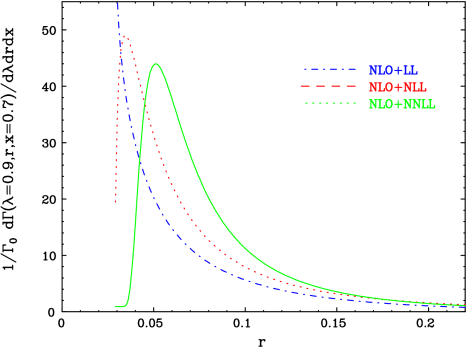
Figure 1: The differential spectrum based on the fixed–logarithmic–accuracy formula of Eq. (3.2), which is matched to NLO. The LL, NLL and NNLL accuracy results are plotted as dotdashed, dashed and full line, respectively. The three curves end at $r\simeq 0.028$, where the resummed results become complex owing to the Landau singularity at $\omega=1/2$.

Fig. 1 shows the differential spectrum as a function of $r$, for the chosen values of $\lambda=0.9$ and $x=0.7$, computed as a derivative of the resummed spectrum in Eq. (3.2). The large differences between curves corresponding to increasing logarithmic accuracy demonstrate the problematic nature of this expansion, in which infrared renormalons (in particular the one at $u=\frac{1}{2}$) are unregulated. This problem is solved in what follows by computing the moment–space Sudakov exponent using Borel summation.

Calculation of the Sudakov factor by Borel summation

Direct evaluation of the Borel integral in the Sudakov exponent of Eq. (35) using the Principal–Value prescription makes optimal use of the known all–order structure of the exponent. In the context of DGE for inclusive spectra, this regularization has been proven effective in several respects [31]:

• No Landau singularities are present.

• It provides a systematic definition of the perturbative sum. Using this definition, cancellation of ambiguities can be realized — this has been explicitly used for the leading renormalon ambiguity associated with the pole mass.

• The Sudakov factor is a real–valued function of the moment variable.

• The resummed spectra has modified support properties. With the appropriate $B_{\cal S}(u)$ (see below), the support is close to that of the physical non-perturbative distribution.

The calculation of the Borel sum in Eq. (35) in a given regularization for the renormalons, requires, in principle, the knowledge of $B_{\cal S}(u)$ and $B_{\cal J}(u)$ for any positive $u$. In contrast to the large–$\beta_{0}$ limit (3.2), analytic expressions for these functions in QCD are not known. The fixed–logarithmic–accuracy approach described above uses only the expansion of these functions, as well as factors $\Gamma(-2u)$ and $\Gamma(-u)$ that multiply them, around the origin ($u=0$). As discussed in detail in Sec. 2.3 in Ref. [31], one may use additional information on the Borel functions $B_{\cal S}(u)$ and $B_{\cal J}(u)$ to constrain further the Sudakov factor. Most importantly, $B_{\cal S}(u)$ at $u=\frac{1}{2}$ was determined in Ref. [31] with a good accuracy using the cancellation [30] of the leading infrared renormalon ambiguity in the Sudakov factor with that of the pole mass.

To understand the origin of renormalons in the Sudakov factor note that the integration over $r$ near the $r\longrightarrow 0$ limit necessarily involves some contribution from the infrared region. ¿From Eq. (36) it is obvious that for small $r$ the coupling is evaluated at small momentum scales, where it is out of perturbative control. In the Borel formulation, when computing the moments in Eq. (3.2) where the integrand is given by Eq. (3.2), the integration gives rise to the factors $\Gamma(-2u)$ and $\Gamma(-u)$ in the soft and jet parts of the exponent, respectively. These factors contain infrared renormalons poles at integer and half integer values of $u$. This way infrared sensitivity translates into power–like ambiguity of the Borel sum [30, 31, 39, 36, 38, 37], corresponding to powers of $n\Lambda/(\lambda m_{b})$ and $n\Lambda^{2}/(\lambda m_{b})^{2}$ in the soft and jet factors, respectively; the latter are obviously less important than the former. As shown in Refs. [30, 31], the leading power ambiguity on the soft scale proportional to $(n-1)\Lambda/(\lambda m_{b})$, cancels exactly with kinematic power corrections. In the present context such corrections arise when expressing $r$ in terms of the hadronic variables; see Sec. 4.

Subleading power ambiguities on the soft scale, corresponding to powers of $(n\Lambda/(\lambda m_{b}))^{j}$ with $j\geq 3$, are related to the momentum distribution of the $b$ quark in the meson. In principle, these ambiguities are removed only upon including a non-perturbative function, namely an infinite set of power corrections, that makes for the difference between the quark distribution in an on-shell heavy quark and that in a meson. The closer to the endpoint one cuts the distribution, the larger is the weight of high moments, and with it the significance of these power corrections. Our analysis of the ${\bar{B}}\longrightarrow X_{s}\gamma$ decay [31] has shown that if $B_{\cal S}(u)$ is sufficiently constrained (see below) and kinematic power corrections are included, one can determine the photon–energy spectrum to a good accuracy neglecting any additional non-perturbative power corrections.

In principle, the theoretical uncertainty associated with the unknown form of the anomalous dimension $B_{\cal S}(u)$ away from the origin, and the unknown non-perturbative power terms that characterize the quark distribution in the meson are two completely distinct issues. In reality, however, both result in similar, parametrically–enhanced power effects, and are therefore impossible to distinguish phenomenologically.

The approach we take in this paper follows closely what was done in Ref. [31]: starting with the large–$\beta_{0}$ result for $B_{\cal S}(u)$ and $B_{\cal J}(u)$, we include ${\cal O}(u)$ and ${\cal O}(u^{2})$ terms to obtain the exact exponent to NNLO. For $B_{\cal S}(u)$ we further include ${\cal}O(u^{3})$ and higher–order terms so as to match the computed residue of at $u=\frac{1}{2}$, getting

$$B_{\cal S}(u) = {\rm e}^{\frac{5}{3}u}(1-u)\exp\left\{c_{2}u+\frac{1}{2}\left[c_{3}-c_{2}^{2}+\frac{C_{A}}{\beta_{0}}\left(\frac{5}{18}\pi^{2}+\frac{7}{9}-\frac{9}{2}\zeta_{3}\right)\right]u^{2}\right\}\times W(u),$$

$$B_{\cal J}(u) = \frac{1}{2}\,{\rm e}^{\frac{5}{3}u}\left(\frac{1}{1-u}+\frac{1}{1-u/2}\right)\frac{\sin\pi u}{\pi u}\,\times$$

$$\exp{\bigg{\{}c_{2}u+\left[c_{3}-c_{2}^{2}+\frac{C_{A}}{\beta_{0}}\left(\frac{29}{72}\pi^{2}-\frac{43}{72}-5\zeta_{3}\right)+\frac{C_{F}}{\beta_{0}}\left(-\frac{\pi^{2}}{4}+\frac{3}{16}+3\zeta_{3}\right)\right]\frac{u^{2}}{2!}+{\cal O}(u^{3})\bigg{\}}},$$

where $c_{2,3}$ are given in Eq. (2.22) in Ref. [31] and where

$$W(u)\equiv{\rm e}^{t_{1}u+\frac{1}{2}t_{2}u^{2}}\,\left(1-t_{1}u+\frac{1}{2}(t_{1}^{2}-t_{2})u^{2}\right)=1+{\cal O}(u^{3}).$$ (43)

Here $t_{1,2}$ are fixed requiring:

$$B_{\cal S}(u=1/2)\,=\,0.91423\,\pm 3\%\,({\rm computed});\quad B_{\cal S}(u=3/2)\,=\,-0.23366\,\times\,C,$$ (44)

where we used the computed normalization of the leading renormalon residue of the pole mass at $u=\frac{1}{2}$ (see eq. (2.30), (2.36) and (4.8) in [31] with $N_{f}=4$) and an arbitrary normalization constant $C$ at $u=\frac{3}{2}$.

We stress that the ansatz of Eq. (3.2) assumes that $B_{\cal S}(u)$ vanishes at $u=1$ and has no other zeros at positive $u$, as in the large–$\beta_{0}$ limit (3.2). The constraint $B_{\cal S}(u=1)=0$ was found to be quite important [31]. Here we explicitly assume that it holds in the full theory and do not investigate the possibility of it being violated. The vanishing of $B_{\cal S}(u=1)$ implies in particular that the perturbative Sudakov factor of  Eq. (35) is free of ${\cal O}((n\Lambda/(\lambda m_{b}))^{2})$ ambiguities. Thus, after the cancellation of the $u=\frac{1}{2}$ ambiguity, the leading ambiguity is ${\cal O}((n\Lambda/(\lambda m_{b}))^{3})$, as already mentioned. To the extent that renormalons do indeed give good indication of which non-perturbative effects are important, the absence of the $u=1$ renormalon is well supported by the successful comparison of the prediction for the first two cut moments in ${\bar{B}}\longrightarrow X_{s}\gamma$ with experimental data.

Note also that Eq. (3.2) tends to zero at asymptotically large $u$. In this respect it differs from the large–$\beta_{0}$ limit. It is important to stress though that convergence of the Borel integrals at large $u$ is guaranteed independently of this assumption, owing to the factors $\Gamma(-2u)$ and $\Gamma(-u)$ in Eq. (35).

In Eq. (3.2) we parametrize $B_{\cal S}(u)$ at intermediate $u$ values by a single parameter $C$. When $B_{\cal S}(u)$ is inserted into Eq. (35) this number determines the renormalon residue at $u=\frac{3}{2}$. The effect of $C$ on the function $B_{\cal S}(u)$ is shown if Fig. 2.

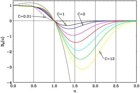
Figure 2: The function $B_{\cal S}(u)$ with vertical lines indicating the positions of possible renormalons owing to the poles of $\Gamma(-2u)$ in Eq. (35). The thin line shows the large–$\beta_{0}$ limit of Eq. (3.2) while the thick lines show $B_{\cal S}(u)$ according to Eq. (3.2) with $N_{f}=4$ and with different assignments of the parameter $C$ that controls the residue of the Borel singularity in the Sudakov exponent at $u=\frac{3}{2}$: $C=0.01$ is shown as a dotdashed line while the default value $C=1$ and $C=2,4,6,8,10,12$ are shown as full lines.

While the actual residue in the full theory is not known, it is expected to be smaller than in the large–$\beta_{0}$ limit, where $B_{\cal S}(u=3/2)\simeq-6.09$. Such a large residue can be obtained in the ansatz of Eq. (3.2) with $N_{f}=4$ by setting $C\simeq 26$ ($W(3/2)\simeq 20$). In model $(c)$ in Sec. 2.3 of [31], we had $B_{\cal S}(u=3/2)\simeq-0.23366$ corresponding to $C=1$ ($W(3/2)\simeq 0.776$). Here we keep $C$ as a free parameter by which we gauge the theoretical uncertainty in the Sudakov factor. The possible range of values for $C$ is discussed further in Sec. 4.2, where we also study the impact of this parameter on the spectrum and on the measurable partial width, see Fig. 8 and Fig. 9, respectively.

3.3 Matching and predictions for the logarithmic terms at NNLO

Using the definition of the moments in Eq. (3.2) with the NLO expansion of Eq. (22) we have

$$\frac{d\Gamma_{n}(\lambda,x)}{d\lambda dx} \equiv \frac{1}{\Gamma_{0}}\int_{0}^{r_{m}}dr\left(1-r\right)^{n-1}\frac{d\Gamma(\lambda,r,x)}{d\lambda drdx}$$

$$= \int_{0}^{r_{m}}dr\left(1-r\right)^{n-1}\bigg{[}V(\lambda,x)\delta(r)+R(\lambda,r,x)\bigg{]}$$

$$= w_{0}(\lambda,x)+\frac{C_{F}\alpha_{s}(m_{b})}{\pi}\bigg{[}w_{1}(\lambda,x)+K_{1}^{n}(\lambda,x)\bigg{]}+{\cal O}(\alpha_{s}^{2}),$$

where $r_{m}\equiv(1-x)/\lambda$ denotes the maximal value of $r$ and

$$K_{1}^{n}(\lambda,x) \equiv \int_{0}^{r_{m}}dr\left(1-r\right)^{n-1}k_{1}(\lambda,r,x)$$

$$= K_{1}^{n\,\hbox{\tiny sing.}}(\lambda,x)+K_{1}^{n\,\hbox{\tiny reg.}}(\lambda,x).$$

where we split the integration into singular and regular terms for $r\longrightarrow 0$:

$$K_{1}^{n\,\hbox{\tiny sing.}}(\lambda,x) \equiv \int_{0}^{r_{m}}dr\left(1-r\right)^{n-1}k_{1}^{\hbox{\tiny sing.}}(\lambda,r,x)$$ (47)

and

$$K_{1}^{n\,\hbox{\tiny reg.}}(\lambda,x) \equiv \int_{0}^{r_{m}}dr\left(1-r\right)^{n-1}k_{1}^{\hbox{\tiny reg.}}(\lambda,r,x)$$

$$= \int_{0}^{r_{m}}dr\left(1-r\right)^{n-1}\bigg{[}k_{1}(\lambda,r,x)-k_{1}^{\hbox{\tiny sing.}}(\lambda,r,x)\bigg{]}$$

where $k_{1}^{\hbox{\tiny sing.}}(\lambda,r,x)$ and $k_{1}(\lambda,r,x)$ is given by Eq. (25) and Eq. (3.1), respectively. In Appendix B we evaluate $K_{1}^{n\,\hbox{\tiny sing.}}(\lambda,x)$ and $K_{1}^{n\,\hbox{\tiny reg.}}(\lambda,x)$ explicitly. The result for the singular part reads

$$K_{1}^{n\,\hbox{\tiny sing.}}(\lambda,x) = -w_{0}(\lambda,x)\bigg{\{}\frac{1}{2}\left[\frac{\pi^{2}}{6}-\Psi_{1}(n)+\left(\Psi(n)+\gamma_{E}\right)^{2}\right]-\frac{7}{4}(\Psi(n)+\gamma_{E})$$

$$-\sum_{k=0}^{\infty}\frac{(1-r_{m})^{n+k}}{n+k}\bigg{[}\ln(r_{m})+\Psi(n+k)-\Psi(n)\bigg{]}-\frac{7}{4}\sum_{k=0}^{\infty}\frac{(1-r_{m})^{n+k}}{n+k}\bigg{\}},$$

while the regular part is given in Eq. (122).

In order to determine the $n$–independent coefficient that multiplies the Sudakov factor in Eq. (35) at ${\cal O}(\alpha_{s})$,

$$\Delta R^{\infty}(\lambda,x)=\Delta K_{1}^{\infty}(\lambda,x)\frac{C_{F}\alpha_{s}(m_{b})}{\pi}\,+\,{\cal O}(\alpha_{s}^{2}),$$ (50)

we compare the expansion of Eq. (35) with the NLO result of Eq. (3.3). We find that the ${\cal O}(\alpha_{s})$ terms that are not generated by the expansion of the exponent are:

$$\Delta K_{1}^{n}(\lambda,x)=K_{1}^{n}(\lambda,x)-\bigg{[}-{\displaystyle\frac{L^{2}}{2}}+\bigg{(}-\gamma_{E}+{\displaystyle\frac{7}{4}}\bigg{)}\,L\bigg{]}w_{0},$$ (51)

where $L=\ln n$, so

$$\Delta K_{1}^{\infty}(\lambda,x)\equiv\lim_{n\to\infty}\Delta K_{1}^{n}(\lambda,x)=-w_{0}(\lambda,x)\left[\frac{\pi^{2}}{12}+\frac{\gamma_{E}^{2}}{2}-\frac{7}{4}\gamma_{E}\right].$$ (52)

Using this coefficient Eq. (35) yields the following perturbative expansion:

$$\left.\frac{d\Gamma_{n}(\lambda,x)}{d\lambda dx}\right|_{{\rm large}\,\,n} = w_{0}(\lambda,x)+\bigg{\{}\bigg{[}-{\displaystyle\frac{L^{2}}{2}}+\bigg{(}-\gamma_{E}+{\displaystyle\frac{7}{4}}\bigg{)}\,L+-\frac{\gamma_{E}^{2}}{2}-\frac{\pi^{2}}{12}+\frac{7}{4}\gamma_{E}\bigg{]}\,w_{0}(\lambda,x)$$

$$\hskip 40.0pt+w_{1}(\lambda,x)\bigg{\}}\,\frac{C_{F}\alpha_{s}(m_{b})}{\pi}$$

$$+ \bigg{\{}\bigg{[}{\displaystyle\frac{C_{F}^{2}\,L^{4}}{8}}+\bigg{(}\bigg{(}-{\displaystyle\frac{7}{8}}+{\displaystyle\frac{\gamma_{E}}{2}}\bigg{)}\,C_{F}^{2}+\bigg{(}-{\displaystyle\frac{11\,C_{A}}{24}}+{\displaystyle\frac{N_{f}}{12}}\bigg{)}\,C_{F}\bigg{)}\,L^{3}$$

$$+ \bigg{(}\bigg{(}{\displaystyle\frac{11\,C_{A}}{12}}-{\displaystyle\frac{N_{f}}{6}}\bigg{)}\,C_{F}\,\ln\lambda+\bigg{(}-{\displaystyle\frac{21}{8}}\,\gamma_{E}+{\displaystyle\frac{3}{4}}\,\gamma_{E}^{2}+{\displaystyle\frac{49}{32}}+\frac{\pi^{2}}{24}\bigg{)}\,C_{F}^{2}$$

$$+ \bigg{(}\bigg{(}{\displaystyle\frac{\gamma_{E}}{4}}-{\displaystyle\frac{13}{144}}\bigg{)}\,N_{f}+\bigg{(}{\displaystyle\frac{95}{288}}-{\displaystyle\frac{11\,\gamma_{E}}{8}}+{\displaystyle\frac{\pi^{2}}{24}}\bigg{)}\,C_{A}\bigg{)}\,C_{F}\bigg{)}L^{2}$$

$$+ \bigg{(}\bigg{(}\bigg{(}{\displaystyle\frac{7}{12}}-{\displaystyle\frac{\gamma_{E}}{3}}\bigg{)}\,N_{f}+\bigg{(}-{\displaystyle\frac{77}{24}}+{\displaystyle\frac{11\,\gamma_{E}}{6}}\bigg{)}\,C_{A}\bigg{)}\,C_{F}\,\ln\lambda$$

$$+ \bigg{(}{\displaystyle\frac{3}{32}}+{\displaystyle\frac{3}{2}}\,\zeta_{3}-{\displaystyle\frac{13\pi^{2}}{48}}+\frac{49\gamma_{E}}{16}+\frac{\pi^{2}\gamma_{E}}{12}-\frac{21\gamma_{E}^{2}}{8}+\frac{\gamma_{E}^{3}}{2}\bigg{)}\,C_{F}^{2}$$

$$+ \bigg{(}\bigg{(}-{\displaystyle\frac{85}{144}}+{\displaystyle\frac{5}{72}}\,\pi^{2}-{\displaystyle\frac{13}{72}}\,\gamma_{E}+{\displaystyle\frac{1}{4}}\,\gamma_{E}^{2}\bigg{)}\,N_{f}$$

$$+ \bigg{(}{\displaystyle\frac{905}{288}}+{\displaystyle\frac{\pi^{2}\,\gamma_{E}}{12}}+{\displaystyle\frac{95\,\gamma_{E}}{144}}-{\displaystyle\frac{67\,\pi^{2}}{144}}-{\displaystyle\frac{11\,\gamma_{E}^{2}}{8}}-{\displaystyle\frac{1}{4}}\,\zeta_{3}\bigg{)}\,C_{A}\bigg{)}C_{F}\bigg{)}L\bigg{]}w_{0}(\lambda,x)$$

$$+ \bigg{[}-{\displaystyle\frac{L^{2}\,C_{F}}{2}}+\bigg{(}-\gamma_{E}+{\displaystyle\frac{7}{4}}\bigg{)}\,C_{F}\,L\bigg{]}\,C_{F}w_{1}(\lambda,x)\bigg{\}}\left(\frac{\alpha_{s}(m_{b})}{\pi}\right)^{2}+\cdots.$$

All the coefficients of the logs determined here are exact. It is important to emphasize that virtual corrections at one–loop order, $w_{1}(\lambda,x)$, contribute to log terms ($C_{F}^{2}L$ and $C_{F}^{2}L^{2}$) at ${\cal O}(\alpha_{s}^{2})$. Similarly, two-loop virtual corrections, $w_{2}(\lambda,x)$, which are yet unknown, contribute to subleading logarithms at ${\cal O}(\alpha_{s}^{3})$ and beyond.

Complete matching at ${\cal O}(\alpha_{s})$ can be achieved by including ${\cal O}(1/n)$ terms additively, using “R matching”:

$$\left.\frac{d\Gamma_{n}(\lambda,x)}{d\lambda dx}\right|_{\rm matched}=\left[V(\lambda,x)+\Delta K_{1}^{\infty}(\lambda,x)\frac{C_{F}\alpha_{s}(m_{b})}{\pi}+{\cal O}(\alpha_{s}^{2})\right]\,\times$$ (54)

$$\exp\bigg{\{}\frac{C_{F}}{\beta_{0}}\int_{0}^{\infty}\frac{du}{u}\,T(u)\left(\frac{\Lambda^{2}}{m_{b}^{2}\lambda^{2}}\right)^{u}\left[B_{\cal S}(u)\Gamma(-2u)\left({n}^{2u}-1\right)-B_{\cal J}(u)\Gamma(-u)\left({n}^{u}-1\right)\right]\bigg{\}}$$

$$+\left[\Delta K_{1}^{n}(\lambda,x)-\Delta K_{1}^{\infty}(\lambda,x)\right]\frac{C_{F}\alpha_{s}(m_{b})}{\pi}+{\cal O}(\alpha_{s}^{2}/n)$$

or, alternatively in front of the Sudakov factor, using “log-R matching”

$$\left.\frac{d\Gamma_{n}(\lambda,x)}{d\lambda dx}\right|_{\rm matched}=\left[V(\lambda,x)\,+\Delta K_{1}^{n}(\lambda,x)\frac{C_{F}\alpha_{s}(m_{b})}{\pi}+{\cal O}(\alpha_{s}^{2})\right]\times$$ (55)

$$\exp\bigg{\{}\frac{C_{F}}{\beta_{0}}\int_{0}^{\infty}\frac{du}{u}\,T(u)\left(\frac{\Lambda^{2}}{m_{b}^{2}\lambda^{2}}\right)^{u}\,\left[B_{\cal S}(u)\Gamma(-2u)\left({n}^{2u}-1\right)-B_{\cal J}(u)\Gamma(-u)\left({n}^{u}-1\right)\right]\bigg{\}}$$

where the terms missing at ${\cal O}(\alpha_{s}^{2})$ include $n$–independent as well as ${\cal O}(1/n)$ terms.

Converting the expansion in Eq. (3.3) to momentum space we obtain for the log-enhanced contribution to the triple differential width (see Eq. (22)) at this order:

$$\left.R\left(\lambda,r,x\right)\right|_{r\longrightarrow 0} = \left(-C_{F}\,\left(\frac{\ln r}{r}\right)_{*}-{\displaystyle\frac{7}{4}}\left(\frac{1}{r}\right)_{*}\,C_{F}\right)\,w_{0}\left(\lambda,x\right)\,\frac{\alpha_{s}\left(m_{b}\right)}{\pi}$$

$$+ \Bigg{\{}\bigg{\{}{\displaystyle\frac{C_{F}^{2}}{2}}\,\left(\frac{\ln^{3}r}{r}\right)_{*}+\bigg{[}{\displaystyle\frac{21\,C_{F}^{2}}{8}}+\left({\displaystyle\frac{11\,C_{A}}{8}}-{\displaystyle\frac{N_{f}}{4}}\right)\,C_{F}\bigg{]}\,\left(\frac{\ln^{2}r}{r}\right)_{*}$$

$$+ \bigg{[}\left({\displaystyle\frac{11\,C_{A}}{6}}-{\displaystyle\frac{N_{f}}{3}}\right)\,C_{F}\,\mathrm{ln}\left(\lambda\right)+\left({\displaystyle\frac{49}{16}}-{\displaystyle\frac{\pi^{2}}{6}}\right)\,C_{F}^{2}$$

$$+ \left(-{\displaystyle\frac{13\,N_{f}}{72}}+\left({\displaystyle\frac{\pi^{2}}{12}}+{\displaystyle\frac{95}{144}}\right)\,C_{A}\right)\,C_{F}\bigg{]}\,\left(\frac{\ln r}{r}\right)_{*}$$

$$+ \bigg{[}\left({\displaystyle\frac{77\,C_{A}}{24}}-{\displaystyle\frac{7\,N_{f}}{12}}\right)\,C_{F}\,\mathrm{ln}\left(\lambda\right)+\left(-{\displaystyle\frac{\pi^{2}}{6}}-{\displaystyle\frac{3}{32}}-{\displaystyle\frac{1}{2}}\,\zeta_{3}\right)\,C_{F}^{2}$$

$$+ \left(\left({\displaystyle\frac{85}{144}}-{\displaystyle\frac{\pi^{2}}{36}}\right)\,N_{f}+\left({\displaystyle\frac{17\,\pi^{2}}{72}}+{\displaystyle\frac{1}{4}}\,\zeta_{3}-{\displaystyle\frac{905}{288}}\right)\,C_{A}\right)\,C_{F}\bigg{]}\left(\frac{1}{r}\right)_{*}\bigg{\}}w_{0}\left(\lambda,x\right)\mbox{}$$

$$+ \left[-{\displaystyle\frac{7}{4}}\,C_{F}^{2}\left(\frac{1}{r}\right)_{*}-\,C_{F}^{2}\left(\frac{\ln r}{r}\right)_{*}\right]\,w_{1}\left(\lambda,x\right)\Bigg{\}}\left(\frac{\alpha_{s}\left(m_{b}\right)}{\pi}\right)^{2}\!+\!{\cal O}\left(\frac{\alpha_{s}\left(m_{b}\right)}{\pi}\right)^{3}.$$

This expression is useful for checking NNLO calculations. An immediate application is the calculation of the log–enhanced part of partially integrated and single differential distributions. For example, the single differential distribution with respect to $\rho$:

$$\frac{1}{\Gamma_{0}}\frac{d\Gamma(\rho)}{d\rho} = \delta(\rho)\bigg{[}1+\frac{C_{F}\alpha_{s}(m_{b})}{\pi}\left(-\frac{13}{144}-\frac{\pi^{2}}{2}\right)+{\cal O}(\alpha_{s})^{2}\bigg{]}+\bigg{\{}-\left(\frac{\ln(\rho)}{\rho}\right)_{*}-\frac{13}{6}\left(\frac{1}{\rho}\right)_{*}$$ (57)

$$- \rho^{2}(3-2\rho)\ln^{2}(\rho)-\frac{1}{6}\left(2-23\rho-9\rho^{2}+8\rho^{3}\right)\ln(\rho)+\frac{79}{18}+\frac{407}{72}\rho-\frac{367}{24}\rho^{2}$$

$$+ \frac{59}{6}\rho^{3}-\frac{25}{9}\rho^{4}+\frac{11}{24}\rho^{5}-\frac{7}{72}\rho^{6}\bigg{\}}\frac{C_{F}\alpha_{s}(m_{b})}{\pi}$$

$$+ \bigg{\{}\frac{1}{2}C_{F}\left(\frac{\ln^{3}(\rho)}{\rho}\right)_{*}+\bigg{[}\frac{13}{4}C_{F}+\frac{11}{8}C_{A}-\frac{1}{4}N_{f}\bigg{]}\left(\frac{\ln^{2}(\rho)}{\rho}\right)_{*}$$

$$+ \bigg{[}\bigg{(}\frac{355}{72}+\frac{1}{3}\pi^{2}\bigg{)}C_{F}+\bigg{(}\frac{1}{12}\pi^{2}+\frac{25}{24}\bigg{)}C_{A}-\frac{1}{4}N_{f}\bigg{]}\left(\frac{\ln(\rho)}{\rho}\right)_{*}$$

$$+ \bigg{[}\bigg{(}-\frac{3571}{1728}+\frac{61}{72}\pi^{2}+\frac{3}{2}\zeta_{3}\bigg{)}C_{F}+\bigg{(}-\frac{1253}{288}+\frac{1}{4}\zeta_{3}+\frac{13}{48}\pi^{2}\bigg{)}C_{A}$$

$$+ \bigg{(}\frac{113}{144}-\frac{1}{36}\pi^{2}\bigg{)}N_{f}\bigg{]}\left(\frac{1}{\rho}\right)_{*}+{\cal O}(\rho^{0})\bigg{\}}\,C_{F}\,\left(\frac{\alpha_{s}(m_{b})}{\pi}\right)^{2}+\cdots.$$

The ${\cal O}(\alpha_{s}^{2})$ coefficient that is leading in $N_{f}$ was recently computed [34] and it is consistent with Eq. (57). The other coefficients are new.

3.4 Exponentiation beyond logarithms

Let us note that the moment–space function obtained by integrating the $r\longrightarrow 0$ singular terms of the form $r^{-1-2u}$ or $r^{-1-u}$ in Eq. (3.2), which are regularized as $()_{*}$ distributions, is not purely logarithmic. Performing the calculation leading to Eq. (35) above but avoiding any further large–$n$ approximation one obtains the following Sudakov factor:

$${\rm Sud}(m_{b}\lambda,n) = \exp\bigg{\{}\frac{C_{F}}{\beta_{0}}\int_{0}^{\infty}\frac{du}{u}\,T(u)\left(\frac{\Lambda^{2}}{m_{b}^{2}\lambda^{2}}\right)^{u}$$

$$\bigg{[}B_{\cal S}(u)\Gamma(-2u)\left(\frac{\Gamma(n)}{\Gamma(n-2u)}-\frac{1}{\Gamma(1-2u)}\right)$$

$$\hskip 100.0pt-B_{\cal J}(u)\Gamma(-u)\left(\frac{\Gamma(n)}{\Gamma(n-u)}-\frac{1}{\Gamma(1-u)}\right)\bigg{]}\bigg{\}}.$$

Note that to any order in $u$: ${\Gamma(n)}/{\Gamma(n-u)}\simeq n^{u}$ up to constant terms. Thus, upon applying this approximation one returns to Eq. (35). There, only powers of $\ln n$ appear at any given order in $u$, while constants and ${\cal O}(1/n)$ terms are entirely excluded from the exponent and appear only in the matching coefficient. In Eq. (3.4) such terms appear also in the exponent.

It is straightforward to match the Sudakov factor of Eq. (3.4) to NLO. The result is more elegant than when using a “purely logarithmic” Sudakov factor (Eq. (55) or Eq. (54)) because the constants for $n\longrightarrow\infty$, which where included there in the process of matching, appear in Eq. (3.4) as part the exponent. This is true at higher orders too: when using Eq. (3.4), $\Delta R^{\infty}=0$. Consequently, it is just the purely virtual terms $V(\lambda,x)$ (terms proportional to $\delta(r)$, after the $()_{+}$ distributions have been defined) that must be multiplied by the Sudakov factor in order to generate correctly the log–enhanced terms at higher orders. Using Eq. (3.4) with “R matching” we get

$$\left.\frac{d\Gamma_{n}(\lambda,x)}{d\lambda dx}\right|_{\rm matched} = V(\lambda,x)\times{\rm Sud}(m_{b}\lambda,n)+\widetilde{\Delta K_{1}}^{n}(\lambda,x)\frac{C_{F}\alpha_{s}(m_{b})}{\pi}+{\cal O}(\alpha_{s}^{2}),$$ (59)

while with “log-R matching” we get

$$\left.\frac{d\Gamma_{n}(\lambda,x)}{d\lambda dx}\right|_{\rm matched}=\left[V(\lambda,x)\,+\widetilde{\Delta K_{1}}^{n}(\lambda,x)\frac{C_{F}\alpha_{s}(m_{b})}{\pi}+{\cal O}(\alpha_{s}^{2})\right]\times{\rm Sud}(m_{b}\lambda,n).$$ (60)

In both cases:

$$\widetilde{\Delta K}_{1}^{n}(\lambda,x) = w_{0}(\lambda,x)\bigg{\{}\bigg{[}\ln(r_{m})+\frac{7}{4}\bigg{]}\times\sum_{k=0}^{\infty}\frac{(1-r_{m})^{n+k}}{n+k}$$

$$+\sum_{k=0}^{\infty}\frac{(1-r_{m})^{n+k}}{n+k}\bigg{[}\Psi(n+k)-\Psi(n)\bigg{]}\bigg{\}}$$

$$+\sum_{i=-4}^{2}f_{i}(\lambda,x)I_{n+i}(r_{m})+\sum_{i=-3}^{2}\tilde{f}_{i}(\lambda,x)J_{n+i}(r_{m}).$$

where the last line corresponds to $K_{1}^{\hbox{\tiny reg.}}$ obtained in Eq. (122). The definitions of the coefficients $f_{i}(\lambda,x)$ and $\tilde{f}_{i}(\lambda,x)$ and the integrals $I_{n+i}(r_{m})$ and $J_{n+i}(r_{m})$ are summarized in Appendix B.

Recall that all the terms in $\widetilde{\Delta K}_{1}^{n}(\lambda,x)$ are suppressed by at least one power of $1/n$. Note, on the other hand, that for fixed $n$ this matching term contains logarithms of $r_{m}$, which get large for $r_{m}\longrightarrow 0$. In particular, the first moment ($n=1$) is:

$$\widetilde{\Delta K}_{1}^{n=1}(\lambda,x) = w_{0}(\lambda,x)\bigg{\{}-\frac{1}{2}\ln^{2}(r_{m})-\frac{7}{4}\ln(r_{m})\bigg{\}}\,+\,K_{1}^{n=1\,\,\hbox{\tiny reg.}}(\lambda,x),$$ (62)

where $K_{1}^{n=1\,\,\hbox{\tiny reg.}}$ is given in Eq. (B).

It is interesting to study the renormalon structure of the Sudakov factor in Eq. (3.4) and compare it to the simplified version of Eq. (35). Let us examine in some detail the soft function (a similar structure appears on the jet side). As discussed in Sec. 4.1 in Ref. [31], power corrections associated with renormalon ambiguities in the soft function modify the Sudakov factor of Eq. (35) or Eq. (3.4) as follows:

$$\left.{\rm Sud}(m_{b}\lambda,n)\right|_{\hbox{\tiny PV}}\,\longrightarrow\,\left.{\rm Sud}(m_{b}\lambda,n)\right|_{\hbox{\tiny PV}}\times$$ (63)

$$\hskip 40.0pt\exp\left\{\sum_{j=1}^{\infty}\left(\frac{\Lambda}{m_{b}\lambda}\right)^{j}f_{j}^{\hbox{\tiny PV}}\pi\frac{C_{F}}{\beta_{0}}\frac{T(j/2)}{j/2}B_{\cal S}(j/2)R(n,j/2)\right\},$$

where the $n$–dependent residue function in the two cases is

$$R(n,j/2)=\left\{\begin{array}[]{ll}{\displaystyle{\rm Res}\,\Gamma(-2u)\left(n^{2u}-1\right){\bigg{|}}_{u=j/2}}&{\rm for\,\,Eq.}\,\,(\ref{Gamma_n_large_n})\\ {\displaystyle{\rm Res}\,\Gamma(-2u)\left(\frac{\Gamma(n)}{\Gamma(n-2u)}-\frac{1}{\Gamma(1-2u)}\right){\bigg{|}}_{u=j/2}}&{\rm for\,\,Eq.}\,\,(\ref{alt_Sud})\end{array}\right.$$ (66)

and $f_{j}^{\hbox{\tiny PV}}$ are dimensionless non-perturbative parameters of order $1$. PV stands for the Principal Values prescription, which is used to define the perturbative sum on the one hand and the non-perturbative parameters on the other. In Eq. (63) the l.h.s. is regularization prescription dependent, while the r.h.s. is not.

It is important to note that subleading renormalons ${\cal O}\left(\left({\Lambda}/({\lambda m_{b}})\right)^{j}\right)$ corresponding to increasing $j$ have an additional numerical suppression owing to the structure of the Sudakov exponent, namely the fact that

$$\left.{\rm Res}\,\Gamma(-2u)\right|_{u=j/2}=\frac{1}{2}\frac{(-1)^{j+1}}{j!}.$$ (67)

Considering only powers of $n\Lambda/(\lambda m_{b})$ the residue structure of the two exponents is the same. In order to analyze the differences between them at smaller $n$ let us now compare between the residue function $R(n,j/2)$ in the two cases for the first few renormalons at $u=j/2$:

$$\begin{array}[]{lll}u&R(n,j/2)\,\,{\rm for\,\,Eq.}\,\,(\ref{Gamma_n_large_n})&R(n,j/2)\,\,{\rm for\,\,Eq.}\,\,(\ref{alt_Sud})\\ \frac{1}{2}&+\frac{1}{2}(n-1)&+\frac{1}{2}(n-1)\\ 1&-\frac{1}{4}(n-1)(n+1)&-\frac{1}{4}(n-1)(n-2)\\ \frac{3}{2}&+\frac{1}{12}(n-1)(n^{2}+n+1)&+\frac{1}{12}(n-1)(n-2)(n-3)\\ 2&-\frac{1}{48}(n-1)(n+1)(n^{2}+1)&-\frac{1}{48}(n-1)(n-2)(n-3)(n-4)\\ \frac{5}{2}&+\frac{1}{240}(n-1)(n^{4}+n^{3}+n^{2}+n+1)&+\frac{1}{240}(n-1)(n-2)(n-3)(n-4)(n-5).\\ \end{array}$$ (74)

Obviously, using Eq. (3.4) the parametric enhancement of power corrections is not as dramatic as it looks based on Eq. (35). In Eq. (3.4) integer moments are entirely free of certain power–like ambiguities which do show up in Eq. (35): according to the residue structure of Eq. (3.4), for $n=N$, $N$ being a positive integer, only powers $(\Lambda/(\lambda m_{b}))^{j}$ with $j<N$ appear.

A priori, one might expect that all power corrections would become of order one at $n\sim\lambda m_{b}/\Lambda$. Assuming that renormalon ambiguities do indeed give good indication on non-perturbative effects, the factorial suppression of Eq. (67) as well as the $n$ dependence of the residues of Eq. (3.4) imply that power terms are altogether less important and, in contrast with the naive expectation, the power expansion corresponding to higher renormalons in Eq. (63) does not break down.

3.5 Resummed double–differential width with a lepton–energy cut

Since the dependence on the lepton energy fraction $x$ appears in the resummation formula (60) only though the phase–space limits and the matching coefficients but not through the Sudakov factor, it is possible to integrate over $x$ analytically to obtain the double differential width with a cut $x>x_{0}$:

$$\frac{1}{\Gamma_{0}}\frac{d\Gamma(\lambda,r,x>x_{0})}{d\lambda dr}=\int_{c-i\infty}^{c+i\infty}\frac{dn}{2\pi i}\,\frac{d\Gamma_{n}(\lambda,x>x_{0})}{d\lambda}\,\left(1-{r}\right)^{-n}$$ (75)

where, based on Eq. (60),

$$\left.\frac{d\Gamma_{n}(\lambda,x>x_{0})}{d\lambda}\right|_{\rm matched}\equiv\int_{\max\{x_{0},1-\lambda\}}^{1}dx\,\left.\frac{d\Gamma_{n}(\lambda,x)}{d\lambda dx}\right|_{\rm matched}$$ (76)

$$\hskip 30.0pt=\left[\overline{V}_{r}(\lambda,x>x_{0})\,+\overline{\Delta K_{1}}^{n}(\lambda,x>x_{0})\frac{C_{F}\alpha_{s}(m_{b})}{\pi}+{\cal O}(\alpha_{s}^{2})\right]\times$$

$$\hskip 50.0pt\exp\bigg{\{}\frac{C_{F}}{\beta_{0}}\int_{0}^{\infty}\frac{du}{u}\,T(u)\left(\frac{\Lambda^{2}}{m_{b}^{2}\lambda^{2}}\right)^{u}\,\bigg{[}B_{\cal S}(u)\Gamma(-2u)\left(\frac{\Gamma(n)}{\Gamma(n-2u)}-\frac{1}{\Gamma(1-2u)}\right)$$

$$\hskip 100.0pt-B_{\cal J}(u)\Gamma(-u)\left(\frac{\Gamma(n)}{\Gamma(n-u)}-\frac{1}{\Gamma(1-u)}\right)\bigg{]}\bigg{\}}.$$

In the Appendix C we explicitly compute the matching coefficients at ${\cal O}(\alpha_{s})$, namely, $\overline{V}_{r}(\lambda,x>x_{0})$ and $\overline{\Delta K_{1}}^{n}(\lambda,x>x_{0})$, by integrating the virtual coefficients of Eq. (22) and the real–emission moments of Eq. (3.4), respectively.

4 Partial width with experimentally relevant cuts in hadronic variables

4.1 Conversion to hadronic variables and power corrections

So far we examined the resummed distribution in kinematic variables associated with the partonic jet initiated by the u-quark. Measurements do not distinguish between the u-quark jet and the soft partons originating in the light degrees of freedom in the meson. Working still in the approximation where the $b$ quark is on shell, one defines $v\equiv p_{B}/M_{B}$ (where $v^{2}=1$) so $p_{b}=m_{b}v$ and the momentum of the light degrees of freedom is $\bar{\Lambda}v=(M_{B}-m_{b})v$. The hadronic variables (in the B rest frame) are then: $E_{H}=E_{j}+\bar{\Lambda}$, where $\bar{\Lambda}=M_{B}-m_{b}$, and $\vec{P}_{H}=\vec{p}_{j}$. The relations with the corresponding hadronic lightcone variables are (cf. Eq. (3.1)):

$$P^{+} = E_{H}-|\vec{P}_{H}|=\bar{\Lambda}+E_{j}-|\vec{p}_{j}|=m_{b}\rho+\bar{\Lambda},$$ (77)

$$P^{-} = E_{H}+|\vec{P}_{H}|=\bar{\Lambda}+E_{j}+|\vec{p}_{j}|=m_{b}\lambda+\bar{\Lambda}.$$

In the small hadronic–mass–squared ($P^{+}P^{-}$) region, $\rho$ is small, and the $\bar{\Lambda}$ term in $P^{+}$ is absolutely essential. On the other hand, the subregion where also $\lambda$ is small ($P^{-}$ is of order $\Lambda$) is unimportant because it is power suppressed by the Born–level weight (see Eq. (131)). Nevertheless, as we carefully treated all other ${\cal O}(\Lambda/m_{b})$ effects, we do not neglect $\bar{\Lambda}$ compared to $m_{b}\lambda$ when converting the decay width to hadronic variables.

In terms of hadronic variables the total phase space is:

$$\Gamma_{\hbox{\tiny total}}=\int_{0}^{M_{B}/2}dE_{l}\int_{M_{B}-2E_{l}}^{M_{B}}dP^{-}\int_{0}^{M_{B}-2E_{l}}dP^{+}\,\,\frac{d\Gamma(P^{+},\,P^{-},\,E_{l})}{dP^{+}\,dP^{-}\,dE_{l}}.$$ (78)

A perturbative calculation of the differential width obviously cannot fill the entire hadronic phase space. The fixed–order perturbative result simply has a smaller phase space, cf. Eq. (19). However, resummation can, and indeed does modify the support properties, violating energy and momentum conservation which hold order by order. In this respect it is essential to distinguish between the region targeted by the resummation and other phase–space regions:

• In the small $P^{+}$ region (or, equivalently, the small hadronic mass region) the resummation dramatically improves the description of the differential width, and with it the support properties. The resummed perturbative distribution of Eq. (34) extends to negative $r$ values. In terms of hadronic variables, the differential width extends to the region $P^{+}<\bar{\Lambda}$ and approximately vanishes for $P^{+}<0$ (see Fig. 3), consistently with the physical support properties [31].

• Away from the region targeted by the resummation, partonic phase–space boundaries are also violated. This, however, is an artifact of uncontrolled ${\cal O}(1/n)$ higher–order perturbative corrections, which depend on the specific scheme by which matching to the fixed–order result is done. As shown in Fig. 3 the phase–space limit $r<(1-x)/\lambda$ (see Eq. (19)) is violated. Fortunately, this makes just a small impact on the observables we consider. This issue is discussed further in Sec. 4.2.

Figure 3: The fully differential width (in units of $\Gamma_{0}$) computed based on Eq. (60), plotted as a function of the small lightcone component $P^{+}$ at $P^{-}=3.5$ GeV and at three different values of $E_{l}=1,\,1.5$ and $2$ GeV. The maximal $P^{+}$ endpoint ($M_{B}-2E_{l}$), denoted by a vertical line, should be: $3.3$, $2.3$ and $1.3$ GeV, respectively. The $u=3/2$ renormalon residue parameter in Eq. (3.2) (see Fig. 2) is $C=1$. Note that the perturbative support properties, namely $\bar{\Lambda}<P^{+}<M_{B}-2E_{l}$ are violated at both ends. At the low $P^{+}$ end this is of course a desired consequence of the resummation: the physical support properties $P^{+}>0$ are approximately recovered. At the high $P^{+}$ end this is an ${\cal O}(\alpha_{s}^{2}/n)$ artifact, which is non-negligible only for large $E_{l}$.

Considering other phase–space limits of $x=2E_{l}/m_{b}$ or $\lambda=(P^{-}-\bar{\Lambda})/m_{b}$ that are not related to the resummation variable $r$, the partonic phase–space limits of Eq. (19) are unmodified by the resummation. The phase space after the $P^{+}$ integration is shown in Fig. 4, where we indicate both the hadronic and the partonic upper limits on the charged lepton energy.

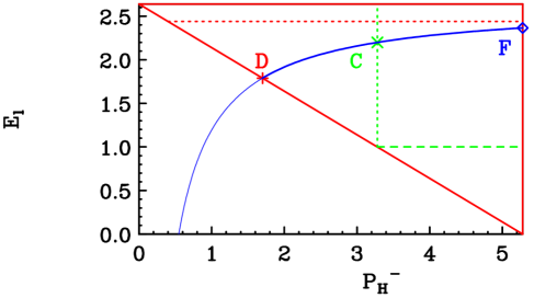
Figure 4: The full phase space in the ($P^{-}$, $E_{l}$) plain (upper left triangle) after the $P^{+}$ integration has been performed. The dotted horizontal line $E_{l}=m_{b}/2$ starting at $P_{H}^{-}=\bar{\Lambda}$ is the upper boundary of the partonic phase space. A lower cut on the charged lepton energy (here $E_{l}>E_{0}=1\,{\rm GeV}$) removes the small triangular region below the horizontal dashed line. An upper cut on the hadronic invariant mass (here $P^{+}P^{-}<M_{X}^{2}=(1.7\,{\rm GeV})^{2}$) affects the distribution for $E_{l}<\frac{1}{2}(M_{B}-M_{X}^{2}/P^{-})$. A full line separates between this region and the rest of the phase space where this cut is irrelevant. On this line we denoted three special points by $D$ $(P^{-}=M_{X})$, $C$ ($P^{-}=M_{B}-2E_{0}$) and $F$ ($P^{-}=M_{B}$), respectively.

As explained below, the transformation of the resummed distribution in the small lightcone component from partonic to hadronic variables has a crucial role in obtaining a correct, unambiguous result (which is also characterized by approximate physical support properties).

To this end, let us recall some of the observations of Refs. [30, 39] and reformulate them in the context of the semileptonic decay. The first observation, already discussed above, is that renormalons in the soft function of Eq. (35) have residues proportional to inverse integer powers of the soft scale, indicating potential non-perturbative power corrections of the form $(n\Lambda/(\lambda m_{b}))^{j}$, where $j$ is a positive integer. It was also observed there that the dominant part of these corrections should be attributed to kinematic effects associated with the mass difference between the meson and the quark, $\bar{\Lambda}=M_{B}-m_{b}$. In the present context these correspond to identifying $r\equiv p_{j}^{+}/p_{j}^{-}=\rho/\lambda$ in terms of hadronic variables using Eq. (77):

$$r=\frac{P^{+}-\bar{\Lambda}}{P^{-}-\bar{\Lambda}},$$ (79)

which effectively shifts the distribution in $r$ by $\bar{\Lambda}/(\lambda m_{b})$. Note that Eq. (77) relies on the assumption that the b quark is on-shell, so this transformation is purely kinematic and the “primordial” motion of the b quark in the meson is not taken into account. In order to account for such non-perturbative dynamics, additional power corrections of the form $(n\Lambda/(\lambda m_{b}))^{j}$ with $j\geq 2$ should be included, as discussed below.

Still within the on-shell heavy–quark approximation, converting Eq. (34) to hadronic variables using Eq. (77) one obtains:

$$\frac{1}{\Gamma_{0}}\frac{d\Gamma(P^{+},\,P^{-},\,E_{l})}{dP^{+}\,dP^{-}\,dE_{l}}=\frac{2}{m_{b}^{2}}\,\frac{1}{P^{-}-\bar{\Lambda}}\,\int_{c-i\infty}^{c+i\infty}\frac{dn}{2\pi i}\,\frac{d\Gamma_{n}(\lambda,x)}{d\lambda dx}\,\,\left(1-\frac{P^{+}-\bar{\Lambda}}{P^{-}-\bar{\Lambda}}\right)^{-n}\times$$

$$\hskip 180.0pt\frac{d\Gamma_{n}(\lambda=\frac{P^{-}-\bar{\Lambda}}{m_{b}},x=\frac{2E_{l}}{m_{b}})}{d\lambda dx}$$ (80)

$$=\,\frac{2}{m_{b}^{2}}\,\frac{1}{P^{-}}\int_{c-i\infty}^{c+i\infty}\frac{dn}{2\pi i}\,\left(1-\frac{\bar{\Lambda}}{P^{-}}\right)^{n-1}\left(1-\frac{P^{+}}{P^{-}}\right)^{-n}\frac{d\Gamma_{n}(\lambda=\frac{P^{-}-\bar{\Lambda}}{m_{b}},x=\frac{2E_{l}}{m_{b}})}{d\lambda dx},$$

where no further approximation was made. The $\bar{\Lambda}$ dependence associated with the shift in $P^{+}$ factorizes exactly in these variables. Note, in particular, that the kinematic power correction factor $\left(1-{\bar{\Lambda}}/{P^{-}}\right)^{n-1}$ is valid for any $n$, not just for large $n$. Obviously, it makes no impact of the first moment and it becomes increasingly important as $n$ gets large.

It was further shown in Ref. [30] that the product

$$\frac{d\Gamma_{n}(\lambda,x)}{d\lambda dx}\,\left(1-\frac{\bar{\Lambda}}{P^{-}}\right)^{n-1}\simeq\frac{d\Gamma_{n}(\lambda,x)}{d\lambda dx}\,\exp\left\{-\frac{(n-1)\bar{\Lambda}}{P^{-}}\right\}(1+{\cal O}(\Lambda/P^{-}))$$ (81)

is free of the leading renormalon ambiguity, a linear ambiguity of ${\cal O}\left(\Lambda(n-1)/P^{-}\right)$ in the exponent, owing to exact cancellation of the $u=\frac{1}{2}$ ambiguities between the Sudakov factor in the resummed moments and the one in $\bar{\Lambda}$. The exponentiation of the corresponding power–like ambiguity in Eq. (35) and the regularization of $\bar{\Lambda}$ and of the Sudakov exponent using the same prescription are crucial for this cancellation to take place. In the Principal Value prescription the numerical result for $\bar{\Lambda}$ is

$$\bar{\Lambda}\equiv\bar{\Lambda}_{\hbox{\tiny PV}}\equiv M_{B}-m_{b}^{\hbox{\tiny PV}}=5.28-4.88\pm 0.06\,{\rm GeV}\,=\,0.40\pm 0.06\,{\rm GeV},$$ (82)

where we used the result for the mass ratio in Eq. (6) with the short–distance quark mass value of Eq. (13) and $N_{f}=4$.

Let us address now power corrections associated with the dynamical structure of the meson. The perturbative calculation of the soft Sudakov exponent accounts for radiation off the heavy quark that puts it slightly off its mass shell. However, it cannot take into account the way in which the virtuality of the heavy quark is influenced by its non-perturbative interaction with the light degrees of freedom in the meson. As discussed in Refs. [30, 31], in the present framework such non-perturbative dynamics is reflected in additional power corrections of form $(n\Lambda/(\lambda m_{b}))^{j}$ with $j\geq 2$. The detailed structure of these power corrections can be read off from the renormalon ambiguities of the soft Sudakov exponent. As done explicitly in Eq. (63) each power ambiguity is associated with a new non-perturbative parameter $f_{j}^{\hbox{\tiny PV}}$; upon including the power term, the corresponding ambiguity is removed. The multiplicative correction to the Sudakov factor in Eq. (63) translates directly into a multiplicative correction to partonic moments computed, for example, in Eq. (60). Given the kinematic cancellation of the leading ($u=1/2$) renormalon ambiguity discussed above, and given that $B_{\cal S}(u=1)$ vanishes (see Eq. (3.2) and the discussion following it), the leading dynamical power correction is associated with the $u=3/2$ ambiguity, corresponding to $j=3$. This correction would modify the spectral moments by

$$\left.\frac{d\Gamma_{n}(\lambda,x)}{d\lambda dx}\right|_{\hbox{\tiny PV}}\,\longrightarrow\,\left.\frac{d\Gamma_{n}(\lambda,x)}{d\lambda dx}\right|_{\hbox{\tiny PV}}\times$$ (83)

$$\hskip 20.0pt\exp\left\{\left(\frac{\Lambda}{m_{b}\lambda}\right)^{3}f_{3}^{\hbox{\tiny PV}}\pi\frac{C_{F}}{\beta_{0}}\frac{T(3/2)}{3/2}B_{\cal S}(3/2)R(n,3/2)\,+\,{\cal O}\left(\left(\frac{\Lambda}{m_{b}\lambda}\right)^{4}\right)\right\},$$

where $R(n,3/2)=\frac{1}{12}(n-3)(n-2)(n-1)$. Note that unless the residue of the anomalous dimension $B_{\cal S}(3/2)$ and the non-perturbative coefficient $f_{3}^{\hbox{\tiny PV}}$ are much larger than one, which we consider unlikely, Eq. (83) amounts to a small correction even for $n\sim\lambda m_{b}/\Lambda$.

The corrections of Eq. (83) go beyond our minimal model: here we regularize all the renormalons using the Principal Value prescription and do not include any additional non-perturbative power terms (i.e. we set $f_{j}^{\hbox{\tiny PV}}=0$ for $j\geq 3$). The resulting, essentially perturbative, spectrum of Eq. (4.1) may therefore differ from the measured spectrum by effects of the from of Eq. (83); because of the parametrically small contribution to moments $n\mathrel{\mathchoice{\vbox{\offinterlineskip\halign{$\m@th\displaystyle\hfil#\hfil$\cr<\crcr\sim\crcr} }}{\vbox{\offinterlineskip\halign{$\m@th\textstyle\hfil#\hfil$\cr<\crcr\sim\crcr} }}{\vbox{\offinterlineskip\halign{$\m@th\scriptstyle\hfil#\hfil$\cr<\crcr\sim\crcr} }}{\vbox{\offinterlineskip\halign{$\m@th\scriptscriptstyle\hfil#\hfil$\cr<\crcr\sim\crcr} }}}\lambda m_{b}/\Lambda$, these effects are restricted to a narrow region near $P^{+}\simeq 0$. We shall revisit this issue in Sec. 4.2 below when estimating the related theoretical uncertainty.

In Appendix D we explicitly show how the resummed result for the spectrum, computed in the previous section using moments of the partonic lightcone momentum ratio $r=\rho/\lambda$, is used to compute the partial branching fraction with experimentally–relevant cuts. In Sec. D.1 we use the results of Sections 3.3 and 3.4 to express the partially integrated width with a cut on $M_{X}$ (or on $P^{+}$) and an additional mild cut on the lepton energy. In Sec. D.2 we derive expressions for the same observables using the results of Sec. 3.5 and Appendix C, where the cut on the lepton energy is implemented analytically. Numerical results for $R_{\rm cut}$ as a function on $M_{X}$ or $P^{+}$ are presented in Sec. 4.2, where we also perform a detailed study of the theoretical uncertainty. Finally, in Sec. 4.3 we extract $|V_{ub}|$ from recent measurements by Belle.

4.2 Numerical results and theoretical uncertainty estimates

In extracting $|V_{ub}|$ from experimental data according to Eq. (2) the effect of kinematic cuts is taken into account through the event fraction $R_{\rm cut}$ defined in Eq. (1). Here we shall use the tools of the previous sections to evaluate $R_{\rm cut}$ for hadronic mass $M_{X}$ or lightcone momentum $P^{+}$ cuts (with additional lower cut on $E_{l}$) and estimate the theoretical uncertainties involved.

It should be emphasized that although the formulae in Sections D.1 and D.2 are explicitly written for partial rates and are normalized by $\Gamma_{0}$, we are really dealing here with the perturbative expansion of $R_{\rm cut}$, not the partial width and the full width separately. A single calculation of $R_{\rm cut}$ in Eq. (1) involves using these formulae twice: with a cut in the numerator, and with no cut in the denominator. Clearly, $\Gamma_{0}$ cancels in the ratio. This has far–reaching implications in what concerns renormalization–scale dependence and renormalon ambiguities: $R_{\rm cut}$, in contrast with the partial (or total) rate in units of $\Gamma_{0}$, is not affected by the ${\cal O}(\Lambda/m_{b})$ renormalon ambiguity. This ambiguity would have cancelled with the ambiguity of $m_{b}^{5}$ in $\Gamma_{0}$ had this factor been included and the series resummed. In $R_{\rm cut}$ it simply cancels between the numerator and the denominator.

As already mentioned, we focus on the cut that maximizes the rate, as measured by Belle [7]: $P^{+}P^{-}<M_{X}^{2}=(1.7\,{\rm GeV})^{2}$ to discriminate the charm background with an additional lepton–energy cut $E_{l}>E_{0}=1$ GeV. Numerical integration of the differential distribution with respect to $P^{-}$ and $E_{l}$, Eq. (151), over the available phase space yields $R_{\rm cut}(M_{X}=1.7\,{\rm GeV},E_{0}=1\,{\rm GeV})=0.615$. This event fraction will be used in the next section to extract $|V_{ub}|$ from Belle data. In this calculation we used the matching of Eq. (60) where the renormalization scale for the coupling was set as $\mu=P^{-}$. In the soft Sudakov exponent we chose $C=1$. In the following we perform a detailed study of the theoretical uncertainty in $R_{\rm cut}$. We consider uncertainties from three sources: (1) higher–order perturbative corrections going beyond the resummation as well as beyond the NLO; (2) renormalons and power corrections, where the main uncertainty is associate with parametrically–enhanced power terms related to the quark distribution in the meson; (3) uncertainty in the values of fundamental short–distance parameters: $\alpha_{s}^{\hbox{\tiny${\overline{\rm MS}}$}}$ and $m_{b}^{\hbox{\tiny${\overline{\rm MS}}$}}$.

Matching schemes, scale dependence and higher–order perturbative effects

The resummation employed here focuses on improving the perturbative expansion of the fully differential width in the particular kinematic region where one lightcone component of the hadronic system, $P^{+}$, is small. Matching has been performed to the full NLO expression. Our purpose here is to estimate the effect of higher–order perturbative corrections on $R_{\rm cut}$. This is done in two ways: first by comparing different matching schemes introduced in sections 3.3 through 3.5, and then by renormalization–scale variation in the matching coefficient.

Let us first estimate the numerical significance of the difference between different matching schemes, which are formally of ${\cal O}(\alpha_{s}^{2}/n)$. Fig. 5 shows the result of three different calculations of the event fraction $R_{\rm cut}$ with a hadronic mass cut $P^{+}P^{-}<M_{X}^{2}$ as a function of $M_{X}$, with a fixed lepton–energy cut $E_{l}>1$ GeV, all with the same choice of renormalization scale for the coupling in the matching coefficient, $\mu=P^{-}$ (see below):

(a) Using the partially integrated distribution with respect to $E_{l}$, namely Eq. (D.2) and Eq. (76).

(b) Using the differential distribution with respect to $E_{l}$, Eq. (151) (or, equivalently, Eqs. (153) through (D.1)) with the matching of Eq. (60).

(c) same as (b) with the matching of Eq. (55).

Figure 5: The event fraction $R_{\rm cut}$ within the range $P^{+}P^{-}<M_{X}^{2}$ and $E_{l}>1$ GeV, plotted as a function of the cut value $M_{X}$. Three different matching schemes are used: (a) the partially integrated distribution with respect to $E_{l}$, namely Eq. (D.2) and Eq. (76), numerically integrated over $P^{-}$ (full line); (b) the fully differential distribution computed by Eq. (151) and the matching of Eq. (60), numerically integrated over the $E_{l}$ and $P^{-}$ (dashed line); and (c) same as in (b) but with the matching of Eq. (55) (dotdashed line).

The origin of the difference between (c) and (b) is clear: the constant terms, which were treated in Eq. (55) as part of the matching coefficient are exponentiated in Eq. (60). Less obvious is the difference between (a) and (b), which is reflected also in the $P^{-}$ distributions plotted in Fig. 6.

Figure 6: The $P^{-}$ distribution after integration over $P^{+}$ (using the moment–space result) and $E_{l}$ in four different situations: no cuts (full line), $E_{l}>1$ GeV cut only (dotdashed line), $E_{l}>1$ GeV combined with $P^{+}P^{-}<M_{X}^{2}=(1.7\,{\rm GeV})^{2}$ cut (dashed), and finally $E_{l}>1$ GeV combined with $P^{+}<P^{+}_{\max}=0.66$ GeV cut (dotted). In each of the two last cases, two different calculation procedures are used in order to gauge the sensitivity to higher–order corrections (matching–scheme dependence): (a) using the partially integrated distribution with respect to $E_{l}$, namely Eq. (D.2) and Eq. (76) and (b) numerically integrating over the differential distribution with respect to $E_{l}$, Eq. (151) and Eq. (60). As explained in the text, the difference between (a) and (b) exists only when there is a $M_{X}$ or a $P^{+}_{\max}$ cut and only for $P^{-}>M_{X}$, or $P^{-}>P^{+}_{\max}$, respectively.

Let us explain this difference for the example where an $M_{X}$ cut is applied.

The first crucial observation is that the resummed distribution (Fig. 3) does not respect the phase space limit $r<(1-x)/\lambda$, which holds order by order in perturbation theory. Instead, the distribution develops a tail that extends up to $r=1$. By construction, the first moment, which is determined by the matching coefficient (i.e. the fixed–order result) alone, is unaffected by this tail. In contrast, whenever one uses the distribution computed as an inverse–Mellin of the resummed moment–space expression these details become important.

Considering next the way the phase space in Fig. 4 is covered we see that in case (a) only the region $P^{-}<M_{X}$ is evaluated using the first moment whereas the entire region $P^{-}>M_{X}$ is reconstructed as an inverse Mellin transform of the resummed expression. In case (b) the differential distribution is used only where necessary: the entire region above the line $E_{l}>\frac{1}{2}(M_{B}-M_{X}^{2}/P^{-})$ is computed using the first moment and only the region below this line depends on the details of the differential distribution. Consequently, (a) effectively uses the distribution (computed as an inverse Mellin transformation) in the region

$$M_{X}<P^{-}<\min\left\{M_{B},\,\frac{M_{X}^{2}}{\bar{\Lambda}}\right\},\qquad E_{l}>\frac{1}{2}\left(M_{B}-\frac{M_{X}^{2}}{P^{-}}\right),$$

where (b) uses the $n=1$ moment instead.

Table 1 summarizes the results corresponding to $P^{+}P^{-}<M_{X}^{2}=(1.7\,{\rm GeV})^{2}$.

matching scheme	Event Fraction $R_{\rm cut}$ ($M_{X}=1.7$ GeV, $E_{0}=1$ GeV)	variation(%)
(a)	0.5941	$-$3.5
(b)	0.6154	default
(c)	0.6364	+3.4

Table 1: Results of the event fraction $R_{\rm cut}$ within the range $M_{X}<1.7$ GeV and $E_{l}>1$ GeV using different matching schemes (see text) with the scale of the coupling in the matching coefficient set as $\mu=P^{-}$.

We see that for the $P^{+}P^{-}<M_{X}^{2}=(1.7\,{\rm GeV})^{2}$ cut, the matching–scheme dependence amounts to less than $\pm 4\%$ uncertainty. Although the fully differential calculation (b) is used to obtain the central value, we will estimate other sources of uncertainty using scheme (a), in which numerical results are obtained faster.

Next, let us consider the renormalization scale dependence. When considering the partial width with stringent cuts, Sudakov resummation is essential. As shown in Refs. [30, 31] and Sec. 3.2 above, the logarithmic accuracy criterion fails because of large running–coupling effects. By using DGE we resum these effects as well. However, this resummation is restricted to the Sudakov exponent. A priori, one might worry that additional resummation of running–coupling effects should be applied in the matching coefficient as well. Using scale variation we show below that this resummation is probably not necessary for the calculation of $R_{\rm cut}$ at the $\pm 5\%$ level.

When considering $R_{\rm cut}$ with very mild cuts Sudakov resummation is irrelevant. But running–coupling effects, which we have not resummed, may still be significant. It is important to emphasize, that these effects cannot be estimated using the expansion of the total width, Eq. (2), which in contrast with $R_{\rm cut}$, is affected by the infrared renormalon corresponding to $m_{b}^{5}$. Determination of the BLM scale in $R_{\rm cut}$ requires the knowledge of the matching coefficients of Sec. 3.3 as a function of $\lambda$ and $x$ to ${\cal O}(\alpha_{s}^{2}\beta_{0})$. These calculations have not yet been performed.

We therefore resort to estimating running–coupling effects in the matching coefficients by means of scale variation. A natural scale for the coupling in the matching coefficient is $P^{-}$, which is the hard scale characterizing the hadronic system. $\mu=P^{-}$ will be our default value. Clearly, as good an alternative would be the partonic $p_{j}^{-}$ — this scale appear as the hard scale in Sudakov exponent, see e.g. Eq. (35) or Eq. (39).

Fig. 7 presents the result for the event fraction $R_{\rm cut}$ associated with a hadronic mass cut $P^{+}P^{-}<M_{X}^{2}$ as a function of $M_{X}$ with a fixed lepton–energy cut $E_{l}>1$ GeV, computed according to Eq. (D.2) and Eq. (76), with three different assignments of the renormalization scale $\mu$ in $\alpha_{s}^{\hbox{\tiny${\overline{\rm MS}}$}}(\mu)$ in both the virtual and real–emission contributions to the matching coefficient.

Figure 7: The event fraction $R_{\rm cut}$ within the range $P^{+}P^{-}<M_{X}^{2}$ and $E_{l}>1$ GeV, computed using Eq. (D.2) and Eq. (76), plotted as a function of the cut value $M_{X}$. Different assignments for the argument of the coupling in the matching coefficient are used.

The results for $P^{+}P^{-}<M_{X}^{2}=(1.7\,{\rm GeV})^{2}$ (and $E_{l}>1$ GeV) are also summarized in Table 2. We find that while the coupling varies from $\alpha_{s}(m_{b})\simeq 0.22$ to $\alpha_{s}(m_{b}/2)\simeq 0.29$, i.e. by over $32\%$, $R_{\rm cut}$ varies only by about $8.3\%$.

scale of $\alpha_{s}$	Event Fraction $R_{\rm cut}$ ($M_{X}=1.7$ GeV, $E_{0}=1$ GeV)	variation (%)
$\mu=P^{-}$	0.5941	default
$\mu=m_{b}$	0.6173	+3.9
$\mu=m_{b}/2$	0.5677	$-$4.4

Table 2: Results of the event fraction within the range $P^{+}P^{-}<M_{X}^{2}=(1.7\,{\rm GeV})^{2}$ and $E_{l}>E_{0}=1$ GeV using Eq. (D.2) and Eq. (76) with different assignments for the scale of the coupling in the matching coefficient (the $n=1$ moment).

Let us consider now the default choice of $\mu=P^{-}$. As shown in Fig. 6 the $P^{-}$ distribution in which no $M_{X}$ (or $P^{+}$) cuts are applied is peaked close to $P^{-}\simeq M_{B}$. On the other hand the $M_{X}$ cut suppresses the distribution at the hard–$P^{-}$ end, while it makes no impact on the soft end. Therefore, the choice of matching–coefficient scale as $\mu=P^{-}$ is a priori quite different from $\mu=m_{b}$. Nevertheless, as shown in Table 2 the overall effect of this change on $R_{\rm cut}$ for $P^{+}P^{-}<M_{X}^{2}=(1.7\,{\rm GeV})^{2}$ (and $E_{l}>1$ GeV) is just $\sim 3.9\%$.

Taking into account the scale uncertainty as $\pm 4.4\%$ and combining it in quadrature with the matching scheme dependence estimate of $\pm 3.5\%$, we assign a total theoretical uncertainty of $5.6\%$ in $R_{\rm cut}$ for $M_{X}=1.7$ GeV owing to unknown higher–order corrections. We expect these number would significantly reduce once NNLO calculations of the fully differential width would be completed.

Renormalons and power corrections

Considering the leading, $u=1/2$ renormalon ambiguity, it is essential to distinguish between

• the ${\cal O}(\Lambda/m_{b})$ renormalon in the total width when written in units of $\Gamma_{0}$ (or the $n=1$ moment of the matching coefficient) which cancels by defining $R_{\rm cut}$ as we did, and

• the cut–related leading ${\cal O}((n-1)\Lambda/m_{b})$ renormalon in the Sudakov exponent which makes all the perturbative moments (but $n=1$) ambiguous and generates an ambiguous shift of the normalized distribution.

While the former is canceled in $R_{\rm cut}$ by definition, the latter affects only the partial width (i.e. the numerator in $R_{\rm cut}$) and becomes more significant the deeper the cut is. As discussed in detail in Sec. 4.1, its cancellation [30, 31] requires renormalon resummation in the Sudakov exponent and incorporating the corresponding kinematic power corrections $\left(1-{\bar{\Lambda}}/{P^{-}}\right)^{n-1}$ according to Eq. (4.1). Having full control of the $u=1/2$ renormalon, including the normalization of its residue, and having defined both the Sudakov factor and ${\bar{\Lambda}}$ using the Principal Value prescription, the computed spectrum is free of any ${\cal O}(\Lambda/(\lambda m_{b}))$ artifact of the non-physical on-shell heavy–quark state.

Beyond the $u=1/2$ renormalon the Sudakov factor has subleading power corrections reflecting the non-perturbative dynamics of the b quark in the B meson. As discussed in Refs.[30, 31] and in Sections 3.4 and 4.1 above, these corrections depend on the definition of the perturbative sum applied in the Sudakov exponent. Moreover, the perturbative Sudakov exponent (60) as well as the corresponding renormalon ambiguities (83) depends on the magnitude of the Borel function away from the origin, so the assumptions made on $B_{\cal S}(u)$ are directly relevant. Let us briefly summarize these assumptions:

(1)  We assumed that, as in the large–$\beta_{0}$ limit (3.2), the Borel function $B_{\cal S}(u)$ vanishes at $u=1$ and has no additional zeros. The vanishing of $B_{\cal S}(1)$ implies, in particular, that there is no ambiguity ${\cal O}((n\Lambda/(\lambda m_{b}))^{2})$ in the exponent so the leading correction, corresponding to the $u=3/2$ renormalon ambiguity, takes the form of Eq. (83);

(2)  We assumed that $B_{\cal S}(u)$ gets small at large $u$, although this is not required for the convergence of the Borel integral. To control the contribution from intermediate values of $u$, we included in the ansatz for $B_{\cal S}(u)$ in Eq. (3.2) a single free parameter $C$ which is proportional to $B_{\cal S}(u=3/2)$; see Fig. 2 and Eq. (44). It is difficult to compute $B_{\cal S}(u=3/2)$, but numerically large (as well as extremely small) values of $C$ can probably be excluded by the following considerations: (a) for $C\simeq 26$ the residue at $u=3/2$ would be as large as in the large–$\beta_{0}$, which is unlikely since non-Abelian corrections tend to reduce renormalon residues; (b) given the ansatz of Eq. (44), either large or small values of $C$ imply that $t_{1}$ and $t_{2}$ become unnaturally large, and so do higher–order perturbative corrections to $B_{\cal S}(u)$. Eventually, these can be computed explicitly to further constrain this function.

Having fixed the Borel transform of the anomalous dimensions in Eq. (3.2), we compute the Sudakov exponent of Eq. (3.4) applying the Principal Value prescription to all the Borel singularities. The resulting DGE spectrum displays only small sensitivity to $C$, see discussion below. Therefore, despite the formal dependence on the regularization prescription for the $u=3/2$ and higher renormalons, this resummed spectrum can be directly considered an approximation to the meson decay spectrum. On the theoretical level, this is supported by the following observations [31]:

• According to the renormalon ambiguity pattern, the leading correction corresponds to the third power of $n\Lambda/(\lambda m_{b})$. Eq. (83) implies that for not–too–high moments ($n\mathrel{\mathchoice{\vbox{\offinterlineskip\halign{$\m@th\displaystyle\hfil#\hfil$\cr<\crcr\sim\crcr} }}{\vbox{\offinterlineskip\halign{$\m@th\textstyle\hfil#\hfil$\cr<\crcr\sim\crcr} }}{\vbox{\offinterlineskip\halign{$\m@th\scriptstyle\hfil#\hfil$\cr<\crcr\sim\crcr} }}{\vbox{\offinterlineskip\halign{$\m@th\scriptscriptstyle\hfil#\hfil$\cr<\crcr\sim\crcr} }}}\lambda m_{b}/\Lambda$) the non-perturbative effect is small, and therefore only a narrow region near $P^{+}\simeq 0$ is affected.

• Despite the finite gap between the physical support properties ($P^{+}>0$) and the perturbative ones ($P^{+}>\bar{\Lambda}$), the resummed perturbative spectrum, quite remarkably, has support that is close to the physical spectrum.

The final judgement, however, must be based on comparison with experimental data. Comparing the predictions of Ref. [31], corresponding to $C=1$ in Eq. (3.2) above, with experimental data for $\bar{B}\longrightarrow X_{s}\gamma$, shows [41] that this minimal model, which essentially has no free parameters, describes the spectrum well. In particular, the first two central moments with cuts, namely the average energy and the width defined with $E_{\gamma}>E_{0}$ (Eqs. (5.3) and (5.4) in Ref. [31]) agree with experiment within error, while for the third moment the data is still statistically limited [12, 13]. It should be emphasized that the theoretical error estimate in [31, 41] did not include any variation of $B_{\cal S}(u)$ nor any non-perturbative power corrections, but only variation of the short–distance parameters $\alpha_{s}^{\hbox{\tiny${\overline{\rm MS}}$}}$ and $m_{b}^{\hbox{\tiny${\overline{\rm MS}}$}}$ within their ranges of uncertainty.

Given the good description of the $\bar{B}\longrightarrow X_{s}\gamma$ spectrum [41] in the present framework, our default choice here is not to include any parametrization of additional non-perturbative corrections of ${\cal O}((n\Lambda/(\lambda m_{b}))^{j})$ with $j\geq 3$. As soon as theoretical predictions and experimental results become sufficiently constraining, parametrization of these corrections along the lines of Eq. (83) would be in place.

We note that since the size of the leading correction in Eq. (83) is controlled by the product of $f_{3}^{\hbox{\tiny PV}}$ and $B_{\cal S}(3/2)$ (or, equivalently, $C$) these two parameters are strongly correlated. Based on data alone it would therefore not be possible to distinguish between genuine non-perturbative effects in the meson ($f_{j}^{\hbox{\tiny PV}}$) and unknown higher–order corrections to $B_{\cal S}(u)$ that modify its behavior away from the origin with respect to Eq. (3.2). To determine $f_{j}^{\hbox{\tiny PV}}$, one would need not only very accurate data but also further theoretical constraints.

Let us therefore proceed by analyzing the numerical consequences of varying $B_{\cal S}(u)$ in Eq. (3.4) by means of $C$, while setting $f_{j}^{\hbox{\tiny PV}}$ ($j\geq 3$) in Eq. (83) to zero. Later we shall consider the uncertainty associated with a non-zero $f_{3}^{\hbox{\tiny PV}}$. $C$ influences the width of the spectrum as a function of $P^{+}$, but even more, the left–right asymmetry in the shape. This can be seen in Fig. 8, where it is also obvious that large values of $C$, such as $C=10$, are disfavored as the distribution extends then further into the negative $P^{+}$ domain, violating the physical support properties.

Figure 8: The fully differential width (in units of $\Gamma_{0}$) computed based on Eq. (60), plotted as a function of the small lightcone component $P^{+}$ at $E_{l}=1.5$ GeV and $P^{-}=3.5$ GeV, for three different assignments of the $u=3/2$ renormalon residue parameter $C$ in Eq. (3.2) (see Fig. 2). $C=1$ is the value used in Ref. [31].

The final effect of varying $C$ within the range $0.1$ to $10$ on $R_{\rm cut}$ is shown in Fig. 9 as a function of $M_{X}$. Results for the experimentally–relevant value of $P^{+}P^{-}<M_{X}^{2}=(1.7\,{\rm GeV})^{2}$ (and $E_{l}>E_{0}=1$ GeV) are also summarized in Table 3. We find that varying $C$ from $0.1$ to $10$ the event fraction varies by only $2.4\%$. Note that the variation is non-monotonous.

$C$	Event Fraction $R_{\rm cut}$ ($M_{X}=1.7$ GeV, $E_{0}=1$ GeV)	variation (%)
$0.1$	0.5799	$-$2.4
$1$	0.5941	default
$10$	0.5870	$-$1.2

Table 3: Results of the event fraction within the range $P^{+}P^{-}<M_{X}^{2}=(1.7\,{\rm GeV})^{2}$ GeV and $E_{l}>1$ GeV using Eq. (D.2) and Eq. (76) with different assignments of $C$ in Eq. (44).

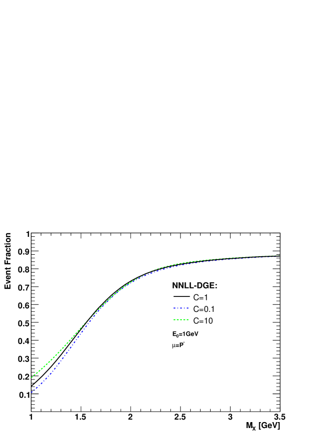
Figure 9: The event fraction $R_{\rm cut}$ within the range $P^{+}P^{-}<M_{X}^{2}$ and $E_{l}>1$ GeV, computed using Eq. (D.2) and Eq. (76), plotted as a function of the cut value $M_{X}$. Different assignments for the unknown parameter $C$, which controls the shape of the perturbative quark distribution function (see Eq. (44)) are used. In the matching coefficient the renormalization scale $\mu=P^{-}$ is chosen.

Finally, let us return to the numerical effect of the leading non-pertrbative correction in Eq. (83). As discussed above, one expects $f_{j}^{\hbox{\tiny PV}}$ to be of ${\cal O}(1)$. For $f_{3}^{\hbox{\tiny PV}}=1$ and for our default value $C=1$ the effect is very small. For example, for the experimentally–relevant cut value of $P^{+}P^{-}<M_{X}^{2}=(1.7\,{\rm GeV})^{2}$ the correction to $R_{\rm cut}$ is $\sim 0.2\%$; naturally, the effect increases significantly when lowering the cut, for example, for $P^{+}P^{-}<M_{X}^{2}=(1.4\,{\rm GeV})^{2}$ it amounts to $1.3\%$. As obvious from Eq. (83), if one assumes $C=10$ instead, the corrections are larger. In this case with $f_{3}^{\hbox{\tiny PV}}=1$ one obtains $0.8\%$ and $4.0\%$ for the two cuts, respectively. Given how small the effect from varying $f_{3}^{\hbox{\tiny PV}}$ is, and its strong correlation with the variation of $C$, we do not include it in the overall uncertainty estimate for $R_{\rm cut}$.

Parametric Uncertainty

The numerical values reported above depend on two short distance parameters, $m_{b}^{\hbox{\tiny${\overline{\rm MS}}$}}$ and $\alpha_{s}^{\hbox{\tiny${\overline{\rm MS}}$}}$. Our default values are $m_{b}^{\hbox{\tiny${\overline{\rm MS}}$}}=4.19$ GeV corresponding to a pole mass of $m_{b}\equiv m_{b}^{\hbox{\tiny PV}}=4.88$ GeV and $\alpha_{s}^{\hbox{\tiny${\overline{\rm MS}}$}}(m_{Z})=0.119$ corresponding to $\alpha_{s}^{\hbox{\tiny${\overline{\rm MS}}$}}(m_{b})=0.217$. The number of light flavors was set as $N_{f}=4$.

To estimate the uncertainty in the computed values of $R_{\rm cut}$ we repeat the calculation with different assignments of these parameters. The results are summarized in Table 4.

parameter	Event Fraction $R_{\rm cut}$ ($M_{X}=1.7$ GeV, $E_{0}=1$ GeV)	variation (%)
$\alpha_{s}^{\hbox{\tiny${\overline{\rm MS}}$}}(m_{Z})=0.115$	0.5832	$-1.8$
$\alpha_{s}^{\hbox{\tiny${\overline{\rm MS}}$}}(m_{Z})=0.119$	0.5941	default
$\alpha_{s}^{\hbox{\tiny${\overline{\rm MS}}$}}(m_{Z})=0.122$	0.5986	$0.8$
$N_{f}=3$	0.6008	$+$1.1
$N_{f}=4$	0.5941	default
$m_{b}^{\hbox{\tiny${\overline{\rm MS}}$}}=4.14$	0.5511	$-7.2$
$m_{b}^{\hbox{\tiny${\overline{\rm MS}}$}}=4.19$	0.5941	default
$m_{b}^{\hbox{\tiny${\overline{\rm MS}}$}}=4.24$	0.6325	$+6.5$

Table 4: Results of the event fraction within the range $P^{+}P^{-}<M_{X}^{2}=(1.7\,{\rm GeV})^{2}$ and $E_{l}>1$ GeV using Eq. (D.2) and Eq. (76) with different assignments of the short distance parameters.

Clearly, the largest parametric uncertainty is related to the value of the quark mass.

Uncertainty estimates for $P^{+}<P_{\max}^{+}$ cut

Let us now perform the calculation of $R_{\rm cut}$ with a cut on the small lightcone component $P^{+}$ in addition to a mild cut on the lepton energy ($E_{l}>1$ GeV). As before, the central value is obtained by numerical integration of the differential distribution computed using Eq. (D.1) with the matching of Eq. (60) over the relevant $P^{-}$ and $E_{l}$ phase space, where the renormalization scale in the matching coefficient is set to be $\mu=P^{-}$ and $C=1$. The central value computed this way for $P^{+}<0.66$ GeV and $E_{l}>1$ GeV (as in the Belle measurement [7]) is $R_{\rm cut}=0.535$.

The error analysis completely parallels the one applied for the $M_{X}$ cut. We therefore briefly summarize the results. The matching scheme uncertainty is summarized in Fig. 10. Numerical values for $P^{+}<0.66$ GeV are given in Table 5.

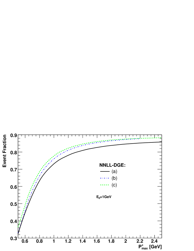
Figure 10: The event fraction $R_{\rm cut}$ within the range $P^{+}<P^{+}_{\max}$ and $E_{l}>1$ GeV, plotted as a function of the cut value $P^{+}_{\max}$. Three different matching schemes are used: (a) the partially integrated distribution with respect to $E_{l}$, namely Eqs. (157) and (D.2) with Eq. (76), numerically integrated over $P^{-}$ (full line); (b) the fully differential distribution computed by Eq. (D.1) and the matching of Eq. (60), numerically integrated over the $E_{l}$ and $P^{-}$ (dashed line); and (c) same as in (b) but with the matching of Eq. (55) (dotdashed line).

matching scheme	Event Fraction $R_{\rm cut}$ ($P^{+}<0.66$ GeV, $E_{l}>1$ GeV)	variation(%)
(a)	0.5118	$-$4.4
(b)	0.5353	default
(c)	0.5659	+5.7

Table 5: Results of the event fraction $R_{\rm cut}$ within the range $P^{+}<P^{+}_{\max}=0.66$ GeV and $E_{l}>1$ GeV using different matching schemes (see Fig. 10 and discussion next to Table 1) with the scale of the coupling in the matching coefficient set as $\mu=P^{-}$.

The renormalization scale dependence in the matching coefficient is shown in Fig. 11.

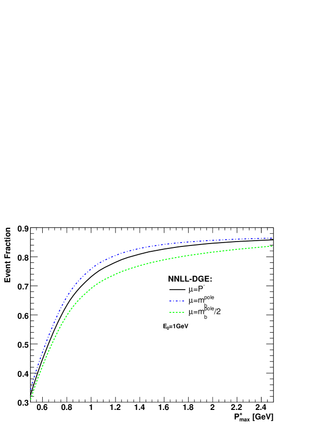
Figure 11: The event fraction $R_{\rm cut}$ within the range $P^{+}<P^{+}_{\max}$ and $E_{l}>1$ GeV, computed using Eqs. (157) and (D.2) and Eq. (76), plotted as a function of the cut value $P^{+}_{\max}$. Different assignments for the argument of the coupling in the matching coefficient are used.

The result for $R_{\rm cut}$ of $P^{+}<P_{\max}^{+}=0.66$ GeV (and $E_{l}>1$ GeV) is summarized in Table 6.

scale of $\alpha_{s}$	Event Fraction $R_{\rm cut}$ for $P^{+}<0.66$ GeV and $E_{l}>1$	variation(%)
$\mu=P^{-}$	0.5118	default
$\mu=m_{b}$	0.5385	+5.2
$\mu=m_{b}/2$	0.4847	$-$5.3

Table 6: Results of the event fraction within the range $P^{+}<0.66$ GeV and $E_{l}>1$ GeV using Eq. (D.2) and Eq. (76) with different assignments for the scale of the coupling in the matching coefficient (the $n=1$ moment).

The total uncertainty due to unknown higher–order corrections amounts to $\pm 7.8\%$, somewhat higher than the uncertainty for the $M_{X}=1.7$ GeV cut, which is 5.6%.

Next, the uncertainty in the shape of the quark distribution function is obtained by modifying $C$ between $C=0.1$ and $C=10$. The result is summarized in Fig. 12 and Table 7.

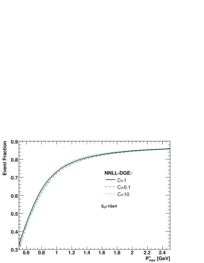
Figure 12: The event fraction $R_{\rm cut}$ within the range $P^{+}<P^{+}_{\max}$ and $E_{l}>1$ GeV, computed using Eqs. (157) and (D.2) and Eq. (76), plotted as a function of the cut value $P^{+}_{\max}$. Different assignments for the parameter $C$, which controls the shape of the perturbative quark distribution function (see Eq. (44)) are used.

$C$	Event Fraction $R_{\rm cut}$ ($P^{+}<0.66$ GeV, $E_{l}>1$ GeV)	variation (%)
$0.1$	0.4971	$-$2.9
$1$	0.5118	default
$10$	0.4909	$-$4.1

Table 7: Results of the event fraction within the range $P^{+}<P^{+}_{\max}=0.66$ GeV and $E_{l}>1$ GeV using Eq. (D.2) and Eq. (76) with different assignments of $C$ in Eq. (44).

Finally, the parametric uncertainty estimates are summarized in Table 8. The total parametric uncertainty is $\pm 12.5$.

parameter	Event Fraction $R_{\rm cut}$ ($P^{+}<0.66$ GeV, $E_{l}>1$ GeV)	variation (%)
$\alpha_{s}^{\hbox{\tiny${\overline{\rm MS}}$}}(m_{Z})=0.115$	0.4922	$-$3.8
$\alpha_{s}^{\hbox{\tiny${\overline{\rm MS}}$}}(m_{Z})=0.119$	0.5118	default
$\alpha_{s}^{\hbox{\tiny${\overline{\rm MS}}$}}(m_{Z})=0.122$	0.5209	+1.8
$N_{f}=3$	0.5207	1.7
$N_{f}=4$	0.5118	default
$m_{b}^{\hbox{\tiny${\overline{\rm MS}}$}}=4.14$	0.4513	$-$11.8
$m_{b}^{\hbox{\tiny${\overline{\rm MS}}$}}=4.19$	0.5118	default
$m_{b}^{\hbox{\tiny${\overline{\rm MS}}$}}=4.24$	0.5650	$+$10.4

Table 8: Results of the event fraction within the range $P^{+}<0.66$ GeV and $E_{l}>1$ GeV using Eq. (D.2) and Eq. (76) with different assignments of the short distance parameters.

In conclusion, when applying a $P^{+}<0.66$ cut instead of a $P^{+}P^{-}<M_{X}^{2}=(1.7\,{\rm GeV})^{2}$ cut the event fraction is reduced by $13\%-14\%$, while the theoretical uncertainty increases. This applies separately to all sources of uncertainty, namely the unknown higher–order corrections (NNLO), the shape of the quark distribution function ($C$) and the values of $\alpha_{s}$ and $m_{b}$.

4.3 Extracting $\left|V_{ub}\right|$

Let us consider first a cut on the invariant mass of the hadronic system, as well as a mild cut on the charged lepton energy, $E_{l}>E_{0}$, as in Ref. [7]. The calculation of the partial branching fraction takes the form:

$$\Delta{\cal B}(\bar{B}\longrightarrow X_{u}l\bar{\nu},P^{+}P^{-}<M_{X}^{2},\,E_{l}>E_{0})$$

$$\hskip 80.0pt=\tau_{B}\Gamma_{\hbox{\tiny total}}\left(\bar{B}\longrightarrow X_{u}l\bar{\nu}\right)R_{\rm cut}(P^{+}P^{-}<M_{X}^{2},\,E_{l}>E_{0}).$$ (84)

The total effect of the cuts amounts to the following event fraction:

$$R_{\rm cut} = \frac{\Gamma(P^{+}P^{-}<(1.7\,{\rm GeV})^{2}\,,\,E_{l}>1\,{\rm GeV})/\Gamma_{0}}{\Gamma(P^{+}P^{-}<M_{B}^{2},\,E_{l}>0)/\Gamma_{0}}$$ (85)

$$= 0.615\pm 0.035_{[\rm higher\,orders]}\pm 0.014_{[{\rm quark\,distribution}]}\pm 0.044_{[{\rm parametric}\,(m_{b}^{\hbox{\tiny${\overline{\rm MS}}$}})]}.$$

Here the central value was computed using numerical integration of the fully differential distribution, Eq. (151) with the matching of Eq. (60) where the renormalization scale was set to $\mu=P^{-}$. The theoretical error estimate was done as explained in Sec. 4.2: the uncertainty associated with higher–order corrections is $\pm 5.6\%$, the one associated with the quark distribution function (renormalons on and power correction on the soft scale) is $\pm 2.4\%$ and the parametric uncertainty (dominated by the uncertainty in $m_{b}$) is $\pm 7.4\%$.

Using Eq. (85) together with the theoretical result for the total charmless semileptonic width of Eq. (2) in Eq. (4.3) with the experimental value of the $B$ lifetime $\tau_{B}=(1.604\pm 0.011)\,{\rm ps}$, and comparing the result to the Belle measurement [7],

$$\Delta{\cal B}(\bar{B}\longrightarrow X_{u}l\bar{\nu},P^{+}P^{-}<(1.7\,{\rm GeV})^{2},\,E_{l}>1\,{\rm GeV})=1.24\cdot 10^{-3}\qquad(\pm 13.4\%)$$ (86)

we get,

$$\left|V_{ub}\right|=\Big{(}4.35\,\pm\,0.28_{[{\rm exp}]}\,\pm\,0.14_{[{\rm th-total}\,(m_{b}^{\hbox{\tiny${\overline{\rm MS}}$}})]}\,\pm\,0.22_{[{\rm th-cuts}]}\Big{)}\cdot 10^{-3},$$ (87)

where the three sources of errors quoted separately are:  (1) the total experimental error [7] on the measured BF in Eq. (86);   (2) the error on the total width, dominated by the uncertainty in $m_{b}^{\hbox{\tiny${\overline{\rm MS}}$}}$ in Eq. (13);   (3) the theory error on the event fraction associated with the hadronic invariant mass cut, computed by adding the three sources of uncertainty in Eq. (85) in quadrature.

Let us consider now the cut on the $P^{+}$ momentum as proposed in [16] and measured in Ref. [7] with $P^{+}<P_{\max}^{+}=0.66$ GeV. The calculation of the partial branching fraction takes the form:

$$\Delta{\cal B}(\bar{B}\longrightarrow X_{u}l\bar{\nu},P^{+}<P_{\max}^{+},\,E_{l}>E_{0})$$

$$\hskip 80.0pt=\tau_{B}\Gamma_{\hbox{\tiny total}}\left(\bar{B}\longrightarrow X_{u}l\bar{\nu}\right)R_{\rm cut}(P^{+}<P_{\max}^{+},\,E_{l}>E_{0}).$$ (88)

The effect of the cuts amounts to the following event fraction:

$$R_{\rm cut} = \frac{\Gamma(P^{+}<0.66\,{\rm GeV}\,,\,E_{l}>1\,{\rm GeV})/\Gamma_{0}}{\Gamma(P^{+}<M_{B},\,E_{l}>0)/\Gamma_{0}}$$ (89)

$$= 0.535\pm 0.042_{[\rm higher\,orders]}\pm 0.021_{[{\rm quark\,distribution}]}\pm 0.063_{[{\rm parametric}\,(m_{b}^{\hbox{\tiny${\overline{\rm MS}}$}})]}.$$

Comparing Eq. (4.3) to the Belle measurement [7],

$$\Delta{\cal B}(\bar{B}\longrightarrow X_{u}l\bar{\nu},P^{+}<0.66\,{\rm GeV}\,,\,E_{l}>1\,{\rm GeV})=1.10\cdot 10^{-3}\qquad(\pm 17.2\%),$$ (90)

we get,

$$\left|V_{ub}\right|=\Big{(}4.39\,\pm\,0.36_{[{\rm exp}]}\,\pm\,0.14_{[{\rm th-total}\,(m_{b}^{\hbox{\tiny${\overline{\rm MS}}$}})]}\,\pm\,0.38_{[{\rm th-cuts}]}\Big{)}\cdot 10^{-3}.$$ (91)

Comparing $\left|V_{ub}\right|$ from the $P^{+}<0.66$ GeV cut in (91) to the one from $P^{+}P^{-}<M_{X}^{2}=(1.7\,{\rm GeV})^{2}$ in (87) and with Ref. [7] we find:

• The central values of $\left|V_{ub}\right|$ we extract using the two cuts agree very well.

• Our results also agree very well with the value quoted by Belle [7] based on their own analysis of the $M_{X}$ cut, while the central value obtained there for the $P^{+}$ cut is $\sim 5\%$ higher.

• The $P^{+}$ cut is characterized by larger theoretical uncertainty; this is even more pronounced than the increase in the experimental error. The largest sources of theoretical uncertainty, for both cuts, are the value of the quark mass and the unknown NNLO corrections.

5 Conclusions

We have presented a calculation of the fully differential distribution in $\bar{B}\longrightarrow X_{u}l\bar{\nu}$ decays that relies only on resummed perturbation theory, and yet describes the meson decay spectrum with approximately correct physical support in the small–$P^{+}$ region. What makes this at all feasible is that the leading renormalon divergence of the Sudakov exponent is fully under control; the corresponding ambiguity of the resummed moments, which amounts to a global ${\cal O}(\Lambda/P^{-})$ shift, cancels out exactly upon converting to hadronic variables, a conversion that itself involves the a priori ambiguous pole-mass definition. While a regularization (Principal Value) has been arbitrarily chosen at the intermediate stage, the end result is unambiguous.

In sharp contrast, an attempt to use Sudakov resummation with fixed logarithmic accuracy — no matter how high — is bound to fail dramatically due to the unregulated renormalon divergence. An example is presented in Figure 13 that compares the DGE spectrum at $E_{l}=1.5$ GeV and $P^{-}=3.5$ GeV to that obtained by standard Sudakov resummation with LL, NLL and NNLL accuracy. Obviously, DGE makes a qualitative difference.

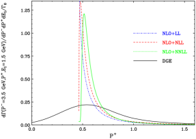
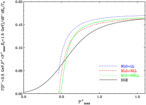
Figure 13: The differential (left) and integrated (right) spectrum based on DGE and on the fixed–logarithmic–accuracy formula of Eq. (3.2), plotted as a function of $P^{+}$. All calculations are matched to NLO. The LL, NLL and NNLL accuracy results are plotted as dotdashed, dashed and full line, respectively. The DGE curve smoothly extends below the partonic phase–space limit, filling up the region $0<P^{+}<\bar{\Lambda}$. In contrast, the three fixed–logarithmic–accuracy curves end above $\bar{\Lambda}$, at the point where the resummed results become complex owing to the Landau singularity.

It should be stressed that the detailed description of the spectrum in the $P^{+}$–peak region, and especially near the $P^{+}=0$ endpoint, is necessarily approximate and it must rely on certain assumptions. First of all, there are both perturbative and non-perturbative contributions. Using moments the latter appear as powers of ${\cal O}(n\Lambda/P^{-})$, so they are parametrically small at small $n$, but they gradually become important as $n$ increases. Uncertainties corresponding to the first and hopefully the second powers of $n\Lambda/P^{-}$ can be avoided — but not the high powers. Towards the small–$P^{+}$ endpoint ($P^{+}\longrightarrow 0$) high moments become relevant and the parametric hierarchy is lost. What dictates the details of the decay spectrum in this region is the quark distribution in the meson. Physically one expects that this distribution would differ from the one in an on-shell quark owing to the interaction between the b quark and the light degrees of freedom. It is our working assumption that these differences are small and therefore better calculation of the latter amounts to better description of the former. Eventually the difference between the two should be quantified.

Non-perturbative contributions aside, computing the on-shell decay spectrum itself within a given regularization scheme for the renormalons is still an incredible task. In Ref. [31] and in the present work we made significant progress in this direction. As we saw, the main difficulty is that the Borel sum in Eq. (3.4) is not entirely dominated by the perturbative expansion in powers of $u$; additional information on the behavior of the Borel integrand away from the origin is needed. Since the general structure of the exponent as a function of $n$ is known, the main uncertainty arises from the soft anomalous dimension function $B_{\cal S}(u)$. The cancellation of the leading renormalon ambiguity with the pole mass allows us to determine $B_{\cal S}(u=1/2)$ accurately [31]. Based on the known analytic result in the large–$\beta_{0}$ limit, we further assumed here that $B_{\cal S}(u=1)=0$ and that this function has no other zeros. We then parametrized the contribution from the region $B_{\cal S}(u\mathrel{\mathchoice{\vbox{\offinterlineskip\halign{$\m@th\displaystyle\hfil#\hfil$\cr>\crcr\sim\crcr} }}{\vbox{\offinterlineskip\halign{$\m@th\textstyle\hfil#\hfil$\cr>\crcr\sim\crcr} }}{\vbox{\offinterlineskip\halign{$\m@th\scriptstyle\hfil#\hfil$\cr>\crcr\sim\crcr} }}{\vbox{\offinterlineskip\halign{$\m@th\scriptscriptstyle\hfil#\hfil$\cr>\crcr\sim\crcr} }}}3/2)$ to facilitate uncertainty estimates. We found that approximately correct non-perturbative support properties are recovered in the Principal Value prescription if this contribution is indeed small. This is demonstrated in Fig. 8.

Under these assumptions we obtained definite predictions for the ${\bar{B}}\longrightarrow X_{s}\gamma$ [31] and $\bar{B}\longrightarrow X_{u}l\bar{\nu}$ spectra. So far comparison with experimental data has been performed for the first two central moments in ${\bar{B}}\longrightarrow X_{s}\gamma$ with varying cuts, finding very good agreement [41]. More detailed comparison of both distributions has a great potential in testing these assumptions and, eventually, in quantifying power corrections.

The fully differential $\bar{B}\longrightarrow X_{u}l\bar{\nu}$ spectrum computed here can be used to extract $|V_{ub}|$ from any experimental measurement of the partial branching fraction. The resummation employed is specifically designed to improve the determination of the partial rate in the small hadronic mass (or small $P^{+}$) region, which is the experimentally–favorable way of discriminating charm. By numerically integrating the differential spectrum over the relevant phase space we computed the fraction of events measured for a given experimental cut. Using recent measurements by Belle [7] for the branching fraction in the regions $P^{+}P^{-}<M_{X}^{2}=(1.7\,{\rm GeV})^{2}$ and $P^{+}<P^{+}_{\max}=0.66$ GeV (with $E_{l}>1\,{\rm GeV}$), we extracted $|V_{ub}|$ and analyzed the theoretical uncertainty. The final results are quoted in Eqs. (87) and (91), respectively. We find that

• The most important source of uncertainty is the value of the b quark mass. It directly influences both the calculation of the total rate and that of the event fraction associated with the cut. Better determination of the mass will therefore translate directly into better measurement of $|V_{ub}|$. One natural possibility for the b quark mass measurement is to make use of recent data on the $\bar{B}\longrightarrow X_{s}\gamma$ spectrum [12, 13] together with calculated spectrum [31].

• Another important source of uncertainty is higher–order perturbative corrections. NNLO calculation of the fully differential $\bar{B}\longrightarrow X_{u}l\bar{\nu}$ is not beyond reach. When available, it can be readily matched to the resummed spectrum. This will significantly reduce the matching scheme dependence as well as the renormalization scale dependence in the matching coefficient.

• Finally, under the assumptions discussed above, the uncertainty associated with the detailed shape of the quark distribution function is found to be quite small. This is most striking in the $M_{X}$ cut, see Fig. 9 and Table 3.

Appendix A Resummation in terms of hadronic and leptonic invariant masses

Let us choose the following kinematic variables [30], all defined at the partonic (perturbative) level:

$$x \equiv 2p_{b}\cdot k_{l}/m_{b}^{2}$$ (92)

$$y \equiv 2p_{b}\cdot q/m_{b}^{2}$$ (93)

$$z \equiv q^{2}/m_{b}^{2}$$ (94)

$$\xi \equiv 1-p_{j}^{2}/m_{b}^{2}=y-z$$ (95)

where momentum conservation implies $p_{b}=p_{j}+q$, where $p_{j}$ is the total momentum of the jet and $q=k_{l}+k_{\nu}$ is the total momentum of the leptons. The total semileptonic width into u-quark is:

$$\Gamma_{\hbox{\tiny total}}=\int_{0}^{1}dz\int_{z}^{1}dx\int_{x-z(1-1/x)}^{1}\!\!\!\!d\xi\,\frac{d\Gamma(z,\xi,x)}{dzdxd\xi}=\Gamma_{0}\,\left[1+\frac{C_{F}\alpha_{s}(m)}{\pi}\left(\frac{25}{8}-\frac{\pi^{2}}{2}\right)+\cdots\right].$$ (96)

where $\Gamma_{0}$ is given by Eq. (21).

NLO result

The perturbative expansion of the triple differential width take the form:

$$\frac{1}{\Gamma_{0}}\frac{d\Gamma(\xi,z,x)}{d\xi dzdx}={\cal V}(z,x)\delta(\xi)+{\cal R}(\xi,z,x)$$ (97)

where

$${\cal V}(z,x) = v_{0}(z,x)+\frac{C_{F}\alpha_{s}(m_{b})}{\pi}v_{1}(z,x)+\cdots,$$ (98)

$${\cal R}(\xi,z,x) = \frac{C_{F}\alpha_{s}(m_{b})}{\pi}d_{1}(\xi,z,x)+\cdots.$$ (99)

The NLO result for the virtual coefficients is:

$$v_{0}(z,x) = 12\,(z+1-x)\,(x-z)$$ (100)

$$v_{1}(z,x) = -12\left(-2\ln(1-z)^{2}-\frac{1}{3}\pi^{2}-\frac{5}{4}-{\rm Li}_{2}(z)\right)(x-z-1)(x-z)$$

$$-6\ln(1-z)(5x-5z-4)(x-z)$$

while the real–emission coefficient is:

$$d_{1}(\xi,z,x) = \bigg{\{}\frac{6\,(x-z-\xi)\,(z-x)\,t\,(z+\xi-2)}{((z+\xi)^{2}-4\,z)^{2}(1-\xi)}\times$$

$$(2\,z^{3}-10\,z^{2}+4\,z^{2}\,\xi-10\,z\,\xi+3\,\xi^{2}\,z+13\,z+\xi^{3}-3\,\xi)$$

$$\mbox{}+{\displaystyle\frac{6\,z\,t\,(z+\xi-2)\,(5-6\,z+2\,z\,\xi+\xi^{2}+2\,z^{2}-4\,\xi)}{((z+\xi)^{2}-4\,z)^{2}}}-6\,(z-x\,z-x\,\xi+x^{2})\,t$$

$$(z+\xi-2)\bigg{[}2\,z^{4}+6\,z^{3}\,\xi-10\,z^{3}+7\,z^{2}\,\xi^{2}+21\,z^{2}-28\,z^{2}\,\xi-14\,\xi^{2}\,z-10\,z$$

$$\mbox{}+4\,z\,\xi^{3}+24\,z\,\xi-5\,\xi^{2}+2\,\xi^{3}+\xi^{4}\bigg{]}\frac{1}{((z+\xi)^{2}-4\,z)^{3}}\bigg{\}}\mathrm{ln}\left({\displaystyle\frac{1+t}{1-t}}\right)$$

$$\mbox{}-{\displaystyle\frac{3\,(7\,z^{2}+4\,z\,\xi-18\,z+6\,\xi+\xi^{2})\,(x-z-\xi)\,(-z+x)}{(-1+\xi)\,((z+\xi)^{2}-4\,z)}}$$

$$\mbox{}+{\displaystyle\frac{3\,z\,(-9\,z+z\,\xi+10+\xi^{2}-3\,\xi)}{((z+\xi)^{2}-4\,z)}}+{\displaystyle\frac{3\,(z-x\,z-x\,\xi+x^{2})}{((z+\xi)^{2}-4\,z)^{2}}}\times$$

$$\hskip 30.0pt\Big{(}11\,z^{3}+17\,z^{2}\,\xi-28\,z^{2}+7\,\xi^{2}\,z+20\,z-38\,z\,\xi+10\,\xi^{2}+\xi^{3}\Big{)}$$

with $t\equiv\sqrt{(z+\xi)^{2}-4z}/(2-z-\xi)$. The $\xi\longrightarrow 1$ singular (non integrable) terms in $d_{1}$, namely

$$d_{1}^{\hbox{\tiny sing.}}=\left[\frac{3(1+z-x)(x-z)}{1-\xi}\left[-4\ln(1-\xi)+8\ln(1-z)-7\right]\right]_{*}$$ (102)

are regularized as $()_{*}$ distributions, as in Eq. (26).

Resummation

The all–order structure of the $\xi\longrightarrow 1$ singular terms in the triple differential width in the large–$\beta_{0}$ limit has been determined in Sec. 3 of Ref. [30] using the Borel technique. The result is summarized by Eq. (30) above. Sudakov resummation can now be performed by exponentiating these singular terms in moment space. Defining moments by

$$\frac{d\Gamma_{N}(z,x)}{dzdx} \equiv \frac{1}{\Gamma_{0}}\int_{x-z(1-1/x)}^{1}d\xi\xi^{N-1}\frac{d\Gamma(\xi,z,x)}{d\xi dzdx}$$

$$\simeq \frac{1}{\Gamma_{0}}\int_{0}^{1}d\xi\xi^{N-1}\left.\frac{d\Gamma(\xi,z,x)}{d\xi dzdx}\right|_{\xi\longrightarrow 1}+{\cal O}(1/N)$$

The singular terms for $\xi\longrightarrow 1$ generate terms that contain powers of $\ln N$, while ${\cal O}(1/N)$ terms are neglected. After matching the resummed distribution can terms can be obtained by the following inverse Mellin formula:

$$\frac{1}{\Gamma_{0}}\frac{d\Gamma(\xi,z,x)}{dzdxd\xi}=\int_{c-i\infty}^{c+i\infty}\frac{dN}{2\pi i}\,\left.\frac{d\Gamma_{N}(z,x)}{dzdx}\right|_{\rm matched}\,\xi^{-N}.$$ (104)

The matched moment–space result takes the form:

$$\left.\frac{d\Gamma_{N}(z,x)}{dzdx}\right|_{\rm matched}=\left[{\cal V}(\lambda,x)\,+\widetilde{\Delta D_{1}}^{N}(\lambda,x)\frac{C_{F}\alpha_{s}(m_{b})}{\pi}+{\cal O}(\alpha_{s}^{2})\right]\times$$ (105)

$$\exp\bigg{\{}\frac{C_{F}}{\beta_{0}}\int_{0}^{\infty}\frac{du}{u}\,T(u)\left(\frac{\Lambda^{2}}{m_{b}^{2}}\right)^{u}\bigg{[}B_{\cal S}(u)(1-z)^{2u}\Gamma(-2u)\left(\frac{\Gamma(N)}{\Gamma(N-2u)}-\frac{1}{\Gamma(1-2u)}\right)$$

$$\hskip 160.0pt-B_{\cal J}(u)\Gamma(-u)\left(\frac{\Gamma(N)}{\Gamma(N-u)}-\frac{1}{\Gamma(1-u)}\right)\bigg{]}\bigg{\}}$$

To perform matching at ${\cal O}(\alpha_{s})$ one needs to compute the moments at this order

$$D_{1}^{N}(\lambda,x) \equiv \frac{1}{\Gamma_{0}}\int_{x-z(1-1/x)}^{1}d\xi\xi^{N-1}\frac{d\Gamma(\xi,z,x)}{d\xi dzdx}\,d_{1}(\xi,z,x),$$ (106)

where $d_{1}(\xi,z,x)$ is given by Eq. (A). We find:

$$D_{1}^{N}(\lambda,x)\! = \!v_{0}(z,x)\bigg{\{}\frac{1}{2}\bigg{[}\Psi_{1}(N)-\frac{1}{6}\pi^{2}-(\gamma_{E}+\Psi(N))^{2}\bigg{]}$$

$$\hskip 30.0pt+\left(\frac{7}{4}-2\ln(1-z)\right)(\Psi(N)+\gamma_{E})\bigg{\}}\,+\,{\cal O}({1}/{N}).$$

These terms, including the constant for $N\longrightarrow\infty$, are reproduced by the expansion of the exponent in Eq. (105), so $\widetilde{\Delta D_{1}}^{N}(\lambda,x)$ contributes only at the level of ${\cal O}(1/N)$ corrections ($\widetilde{\Delta D_{1}}^{\infty}(\lambda,x)=0$). Therefore, Eq. (105) with the coefficients of ${\cal V}(\lambda,x)$ given by Eq. (100) can readily be expanded to predict the log-enhanced terms at ${\cal O}(\alpha_{s}^{2})$. Converting this result back to $\xi$ space, we get:

$$\left.\frac{1}{\Gamma_{0}}\frac{d\Gamma(\xi,z,x)}{dzdxd\xi}\right|_{\xi\longrightarrow 1}\!\!\!\!\! = v_{0}(z,x)+\Bigg{\{}\bigg{[}-\,\left(\frac{\ln(1-\xi)}{1-\xi}\right)_{*}+\left(-{\frac{7}{4}}+2\,\ln(1-z)\right)\,\left(\frac{1}{1-\xi}\right)_{*}\bigg{]}\,\times$$

$$v_{0}(z,x)\,+\,v_{1}(z,x)\Bigg{\}}\frac{C_{F}\alpha_{s}(m_{b})}{\pi}+\Bigg{\{}\bigg{[}\frac{C_{F}^{2}}{2}\,\left(\frac{\ln^{3}(1-\xi)}{1-\xi}\right)_{*}$$

$$+\left(\bigg{(}-3\,\ln(1-z)+{\frac{21}{8}}\bigg{)}\,C_{F}^{2}+\bigg{(}{\frac{11\,C_{A}}{8}-{\frac{N_{f}}{4}}}\bigg{)}\,C_{F}\right)\,\left(\frac{\ln^{2}(1-\xi)}{1-\xi}\right)_{*}$$

$$+\bigg{(}\bigg{(}4\,\ln(1-z)^{2}-{\frac{\pi^{2}}{6}}+{\frac{49}{16}}-7\,\ln(1-z)\bigg{)}\,C_{F}^{2}\mbox{}+\bigg{(}\bigg{(}{\frac{2}{3}}\,\ln(1-z)$$

$$-{\frac{13}{72}}\bigg{)}\,N_{f}+\bigg{(}{\frac{\pi^{2}}{12}}-{\frac{11}{3}}\,\mathrm{ln}(1-z)+{\frac{95}{144}}\bigg{)}\,C_{A}\bigg{)}\,C_{F}\bigg{)}\left(\frac{\ln(1-\xi)}{1-\xi}\right)_{*}\mbox{}$$

$$+\bigg{(}\bigg{(}-{\frac{\pi^{2}}{6}}+{\frac{1}{3}}\,\ln(1-z)\,\pi^{2}-{\frac{3}{32}}-{\frac{1}{2}}\,\zeta_{3}\bigg{)}\,C_{F}^{2}$$

$$+\left(-{\frac{\pi^{2}}{36}}-{\frac{2}{9}}\,\ln(1-z)-{\frac{1}{3}}\,\ln(1-z)^{2}+{\frac{85}{144}}\right)\,C_{F}N_{f}$$

$$\mbox{}+\bigg{(}{\frac{17}{9}}\,\ln(1-z)+{\frac{17\,\pi^{2}}{72}}+{\frac{1}{4}}\,\zeta_{3}+{\frac{11}{6}}\,\ln(1-z)^{2}-{\frac{905}{288}}$$

$$-{\frac{1}{6}}\,\ln(1-z)\,\pi^{2}\bigg{)}\,C_{F}C_{A}\bigg{)}\left(\frac{1}{1-\xi}\right)_{*}\bigg{]}v_{0}(z,x)\mbox{}+\bigg{[}-\left(\frac{\ln(1-\xi)}{1-\xi}\right)_{*}$$

$$+\bigg{(}-{\frac{7}{4}}+2\,\ln(1-z)\bigg{)}\,\left(\frac{1}{1-\xi}\right)_{*}\bigg{]}\,\,C_{F}^{2}\,v_{1}(z,x)\Bigg{\}}\left(\frac{\alpha_{s}(m_{b})}{\pi}\right)^{2}$$

Changing variable in Eq. (A) to the lightcone momenta $\rho$ and $\lambda$ we get

$$\left.\frac{1}{\Gamma_{0}}\frac{d\Gamma(\lambda,\rho,x)}{d\lambda d\rho dx}\right|_{\rho\longrightarrow 0} = v_{0}(z=1-\lambda,x)+\Bigg{\{}\bigg{[}-\,\left(\frac{\ln\rho}{\rho}\right)+\left(\ln(\lambda)-{\frac{7}{4}}\right)\left(\frac{1}{\rho}\right)\bigg{]}\,\times$$

$$v_{0}(z=1-\lambda,x)\,+\,v_{1}(z=1-\lambda,x)\Bigg{\}}\,\left(\frac{C_{F}\,\alpha_{s}(m_{b})}{\pi}\right)+\bigg{\{}\bigg{[}{\frac{1}{2}}\,C_{F}^{2}\,\left(\frac{\ln^{3}\rho}{\rho}\right)$$

$$\mbox{}+\bigg{(}-{\frac{3}{2}}\,C_{F}^{2}\,\ln(\lambda)+{\frac{21\,C_{F}^{2}}{8}}+\left({\frac{11\,C_{A}}{8}}-{\frac{N_{f}}{4}}\right)\,C_{F}\bigg{)}\,\left(\frac{\ln^{2}\rho}{\rho}\right)$$

$$+\bigg{(}-{\frac{1}{2}}\,C_{F}^{2}\,\ln(\lambda)^{2}\mbox{}+\bigg{(}-{\frac{7\,C_{F}^{2}}{4}}+\bigg{(}{\frac{N_{f}}{6}}-{\frac{11\,C_{A}}{12}}\bigg{)}\,C_{F}\bigg{)}\,\ln(\lambda)$$

$$+\bigg{(}-{\frac{\pi^{2}}{6}}+{\frac{49}{16}}\bigg{)}\,C_{F}^{2}+\bigg{(}-{\frac{13\,N_{f}}{72}}+\bigg{(}{\frac{95}{144}}+{\frac{\pi^{2}}{12}}\bigg{)}\,C_{A}\bigg{)}\,C_{F}\bigg{)}\left(\frac{\ln\rho}{\rho}\right)$$

$$+\bigg{(}{\frac{3}{2}}\,C_{F}^{2}\,\ln(\lambda)^{3}\mbox{}+\bigg{(}-{\frac{35\,C_{F}^{2}}{8}}+\left(-{\frac{11\,C_{A}}{24}}+{\frac{N_{f}}{12}}\right)\,C_{F}\bigg{)}\,\ln(\lambda)^{2}$$

$$\mbox{}+\bigg{(}\bigg{(}{\frac{\pi^{2}}{6}}+{\frac{49}{16}}\bigg{)}\,C_{F}^{2}+(-{\frac{29\,N_{f}}{72}}+\bigg{(}{\frac{367}{144}}-{\frac{\pi^{2}}{12}}\bigg{)}\,C_{A})\,C_{F}\bigg{)}\,\ln(\lambda)$$

$$\mbox{}+\bigg{(}-{\frac{\pi^{2}}{6}}-{\frac{1}{2}}\,\zeta_{3}-{\frac{3}{32}}\bigg{)}\,C_{F}^{2}+\bigg{(}\bigg{(}-{\frac{\pi^{2}}{36}}+{\frac{85}{144}}\bigg{)}\,C_{F}N_{f}$$

$$+\left({\frac{1}{4}}\,\zeta_{3}+{\frac{17\,\pi^{2}}{72}}-{\frac{905}{288}}\right)\,C_{F}C_{A}\bigg{)}\,\bigg{)}\left(\frac{1}{\rho}\right)\bigg{]}v_{0}(z=1-\lambda,x)$$

$$\mbox{}+\bigg{[}-\left(\frac{\ln\rho}{\rho}\right)+\left(\ln(\lambda)-{\frac{7}{4}}\right)\left(\frac{1}{\rho}\right)\bigg{]}\,C_{F}^{2}\,v_{1}(z=1-\lambda,x)\bigg{\}}\left(\frac{\alpha_{s}(m_{b})}{\pi}\right)^{2}$$

These logarithms agree exactly with those predicted using the variables $r$ and $\lambda$, Eq. (20) with Eq. (3.3). Note, however, that the separation into virtual and real is different when different variables are used to define the $()_{*}$ distributions.

Appendix B Calculation of the real-emission contribution at NLO in moment space

Singular part

For the singular part of Eq. (47) we get

$$K_{1}^{n\,\hbox{\tiny sing.}}(\lambda,x) = -w_{0}(\lambda,x)\int_{0}^{r_{m}}dr\left(1-r\right)^{n-1}\left[{\displaystyle\frac{\ln(r)+\frac{7}{4}}{r}}\right]_{*}$$

$$= -w_{0}(\lambda,x)\bigg{[}\frac{1}{2}\ln^{2}(r_{m})+i_{0}^{n}(r_{m})+\frac{7}{4}\Big{(}\ln(r_{m})+i_{1}^{n}(r_{m})\Big{)}\bigg{]},$$

where we applied the definition of the $()_{*}$ distribution in Eq. (26) and defined

$$i_{0}^{n}(r_{m}) \equiv \int_{0}^{r_{m}}dr\bigg{[}(1-r)^{n-1}-1\bigg{]}\frac{\ln r}{r}$$

$$= (n-1)r_{m}\bigg{[}\,_{4}F_{3}([1,1,1,2-n],[2,2,2],r_{m})\,-\,\ln(r_{m})\,_{3}F_{2}([1,1,2-n],[2,2],r_{m})\bigg{]}$$

$$= \frac{1}{2}\left[\frac{\pi^{2}}{6}-\Psi_{1}(n)+\left(\Psi(n)+\gamma_{E}\right)^{2}-\ln^{2}(r_{m})\right]\!-\!\ln(r_{m})s_{1}(n,1-r_{m})\!-\!s_{2}(n,1-r_{m})$$

and

$$i_{1}^{n}(r_{m}) \equiv \int_{0}^{r_{m}}dr\bigg{[}(1-r)^{n-1}-1\bigg{]}\frac{1}{r}$$

$$= -r_{m}\,(n-1)\,\times\,_{3}F_{2}([1,1,2-n],[2,2],r_{m})$$

$$= -\Big{[}\ln(r_{m})+\Psi(n)+\gamma_{E}\Big{]}-s_{1}(n,1-r_{m})\,,$$

where $s_{1,2}$ denote the infinite sums:

$$s_{1}(n,1-r_{m}) \equiv \sum_{k=0}^{\infty}\frac{(1-r_{m})^{n+k}}{n+k}$$

$$= \frac{(1-r_{m})^{n}}{n}\,_{2}F_{1}([1,n],[n+1],1-r_{m})=(1-r_{m})^{n}\,{\rm LerchPhi}(1-r_{m},1,n)$$

$$s_{2}(n,1-r_{m}) \equiv \sum_{k=0}^{\infty}\frac{(1-r_{m})^{n+k}}{n+k}\bigg{[}\Psi(n+k)-\Psi(n)\bigg{]}.$$

Alternative expressions, useful for small $r_{m}$, are:

$$s_{1}(n,1-r_{m}) = -\Big{(}\ln(r_{m})+\Psi(n)+\gamma_{E}\Big{)}\,-\,\sum_{k=1}^{\infty}\frac{(-r_{m})^{k}\,\Gamma(n)}{\Gamma(k+1)\,k\,\Gamma(n-k)}$$ (114)

$$s_{2}(n,1-r_{m}) = \frac{1}{2}\Big{(}\ln(r_{m})+\Psi(n)+\gamma_{E}\Big{)}^{2}+\frac{1}{12}\pi^{2}-\frac{1}{2}\Psi_{1}(n)\,+\sum_{k=1}^{\infty}\frac{(-r_{m})^{k}\,\Gamma(n)}{\Gamma(k+1)\,k^{2}\,\Gamma(n-k)}.$$

¿From the definitions of $i_{0,1}$ and Eq. (B) it follows that the first moment ($n=1$) of the singular part, which is relevant for the total width, is simply:

$$K_{1}^{n=1\,\hbox{\tiny sing.}}(\lambda,x) = -w_{0}(\lambda,x)\bigg{[}\frac{1}{2}\ln^{2}(r_{m})+\frac{7}{4}\ln(r_{m})\bigg{]}.$$ (115)

We note that $i_{0,1}^{n}(r_{m})={\cal O}(r_{m})$, so for any moment the small–$r_{m}$ limit ($x\longrightarrow 1$) is particularly simple:

$$K_{1}^{n\,\hbox{\tiny sing.}}(\lambda,x\longrightarrow 1)\longrightarrow K_{1}^{n=1\,\hbox{\tiny sing.}}(\lambda,x\longrightarrow 1).$$

For fixed $r_{m}$ the sums $s_{1,2}(n,1-r_{m})$ in Eq. (B) vanish exponentially at large $n$. Thus, in the final expression in Eqs. (B) and (B) only the square brackets contains terms that do not vanish at $n\longrightarrow\infty$. The logarithms of $r_{m}$ appearing explicitly in Eq. (B) cancel against the ones in $i_{1}$ and $i_{0}$, yielding

$$K_{1}^{n\,\hbox{\tiny sing.}}(\lambda,x) = -w_{0}(\lambda,x)\bigg{\{}\frac{1}{2}\left[\frac{\pi^{2}}{6}-\Psi_{1}(n)+\left(\Psi(n)+\gamma_{E}\right)^{2}\right]-\frac{7}{4}(\Psi(n)+\gamma_{E})$$

$$-s_{1}(n,1-r_{m})\ln(r_{m})-s_{2}(n,1-r_{m})-\frac{7}{4}s_{1}(n,1-r_{m})\bigg{\}},$$

so the $r_{m}$ dependence of $K_{1}^{n\,\hbox{\tiny sing.}}(\lambda,x)$ appears only though ${\cal O}(1/n)$ terms. The terms is the curly brackets in Eq. (B) in the first and second lines can interpreted as originating in the two following integrals, respectively,

$$K_{1}^{n\,\hbox{\tiny sing.}}(\lambda,x) = -w_{0}(\lambda,x)\bigg{\{}\int_{0}^{1}(1-r)^{n-1}\left(\frac{\ln r}{r}+\frac{7}{4}\frac{1}{r}\right)_{*}$$

$$\hskip 100.0pt-\int_{r_{m}}^{1}(1-r)^{n-1}\left(\frac{\ln r}{r}+\frac{7}{4}\frac{1}{r}\right)\bigg{\}}.$$

Regular part

Let us consider now the regular part of Eq. (3.3). The first moment ($n=1$), which is useful in calculating the integrated width, is fairly simple:

$$K_{1}^{n=1\,\,\hbox{\tiny reg.}}(\lambda,x) = 6\,{\rm Li}_{2}\left(1-{\displaystyle\frac{1-x}{\lambda}}\right)\bigg{[}8\,\lambda+36\,\lambda^{5}+232\,\lambda^{3}-190\,\lambda^{4}-90\,\lambda^{2}$$

$$\mbox{}-\bigg{(}4-196\,\lambda^{3}-76\,\lambda+225\,\lambda^{2}+40\,\lambda^{4}\bigg{)}\,(1-x)$$

$$\mbox{}+(34\,\lambda-33\,\lambda^{2}+8\,\lambda^{3}-8)\,(1-x)^{2}\bigg{]}\mbox{}-\ln\left({\displaystyle\frac{1-x}{\lambda}}\right)\,\frac{1-x}{\lambda}\,\bigg{[}216\,\lambda^{5}-1140\,\lambda^{4}$$

$$\mbox{}+84\,\lambda+1416\,\lambda^{3}-612\,\lambda^{2}-3\,\bigg{(}-199\,\lambda^{3}+211\,\lambda^{2}+2-70\,\lambda+44\,\lambda^{4}\bigg{)}\,(1-x)$$

$$\mbox{}-2\,(1-\lambda)\,\bigg{(}\lambda^{2}-2\,\lambda+2\bigg{)}\,(1-x)^{2}\bigg{]}\mbox{}+\frac{1}{6\,\lambda}\bigg{[}540\,\pi^{2}\,\lambda^{3}-216\,\pi^{2}\,\lambda^{6}-1392\,\pi^{2}\,\lambda^{4}$$

$$\mbox{}+1140\,\pi^{2}\,\lambda^{5}-48\,\pi^{2}\,\lambda^{2}\bigg{]}+(1-x)\,\bigg{[}4\,\pi^{2}-516\,\lambda-196\,\pi^{2}\,\lambda^{3}-76\,\pi^{2}\,\lambda$$

$$\mbox{}+225\,\pi^{2}\,\lambda^{2}+216\,\lambda^{4}-1140\,\lambda^{3}+1365\,\lambda^{2}+60+40\,\pi^{2}\,\lambda^{4}\bigg{]}-\frac{(1-x)^{2}}{2\,\lambda}\,\bigg{[}-624\,\lambda$$

$$\mbox{}+39+16\,\pi^{2}\,\lambda^{4}+1995\,\lambda^{2}-1812\,\lambda^{3}+372\,\lambda^{4}-16\,\pi^{2}\,\lambda-66\,\pi^{2}\,\lambda^{3}+68\,\pi^{2}\,\lambda^{2}\bigg{]}$$

$$-\frac{1}{3\,\lambda}\,(1-\lambda)\,\bigg{[}29\,\lambda^{2}-70\,\lambda+43\bigg{]}.$$

To express a general $n$-th moment of the regular part, we write

$$k_{1}^{n\,\hbox{\tiny reg.}}(\lambda,r,x)=\sum_{i=-4}^{2}f_{i}(\lambda,x)(1-r)^{i}\ln(r)+\sum_{i=-3}^{2}\tilde{f}_{i}(\lambda,x)(1-r)^{i},$$ (119)

where we consider $n$ complex with sufficiently large real part, ${\rm Re}(n)>3$, to obtain convergence of the defining moment integral in Eq. (3.3) for individual terms in the sum, and where

$$f_{-4}(\lambda,x) = \,-36\,(\lambda-6)\,(\lambda-1)^{2}\,(\lambda-1+x)^{2}$$ (120)

$$f_{-3}(\lambda,x) = \,36\,(\lambda-1)\,(3\,\lambda^{2}-17\,\lambda+9)\,x^{2}+36\,(7\,\lambda^{2}-40\,\lambda+18)\,(\lambda-1)^{2}\,x$$

$$\mbox{}+36\,(\lambda-1)^{3}\,(4\,\lambda^{2}-23\,\lambda+9)$$

$$f_{-2}(\lambda,x) = \,-6\,(19\,\lambda^{3}-102\,\lambda^{2}-34+112\,\lambda)\,x^{2}$$

$$\mbox{}-12\,(-1+\lambda)\,(29\,\lambda^{3}-159\,\lambda^{2}+148\,\lambda-38)\,x-4008\,\lambda^{3}-1608\,\lambda$$

$$+1812\,\lambda^{4}-240\,\lambda^{5}+252+3792\,\lambda^{2}$$

$$f_{-1}(\lambda,x) = \,6\,(8\,\lambda^{3}-33\,\lambda^{2}-8+34\,\lambda)\,x^{2}+6\,(-212\,\lambda^{3}+291\,\lambda^{2}-144\,\lambda+20+40\,\lambda^{4})\,x$$

$$\mbox{}+2616\,\lambda^{3}+708\,\lambda-1380\,\lambda^{4}+216\,\lambda^{5}-72-2088\,\lambda^{2}$$

$$f_{0}(\lambda,x) = \,-6\,(\lambda-1)\,(\lambda^{2}+2-2\,\lambda)\,x^{2}-6\,(-58\,\lambda^{3}-34\,\lambda+71\,\lambda^{2}+6+14\,\lambda^{4})\,x$$

$$\mbox{}-990\,\lambda^{3}+24-114\,\lambda^{5}+600\,\lambda^{4}-228\,\lambda+708\,\lambda^{2}$$

$$f_{1}(\lambda,x) = \,\,12\,(\lambda-1)\,\lambda\,(\lambda^{2}+2-2\,\lambda)\,x+6\,(\lambda-1)\,\lambda\,(6\,\lambda^{3}-19\,\lambda^{2}+18\,\lambda-6)$$

$$f_{2}(\lambda,x) = \,-6\,\lambda^{2}\,(\lambda-1)\,(\lambda^{2}+2-2\,\lambda)$$

and

$$\tilde{f}_{-3}(\lambda,x) = \,-36\,(\lambda-6)\,(\lambda-1)^{2}\,x^{2}-72\,(\lambda-6)\,(\lambda-1)^{3}\,x+216+360\,\lambda^{4}$$ (121)

$$\mbox{}-36\,\lambda^{5}+1440\,\lambda^{2}-900\,\lambda-1080\,\lambda^{3}$$

$$\tilde{f}_{-2}(\lambda,x) = \,18\,(\lambda-1)\,(5\,\lambda^{2}-27\,\lambda+12)\,x^{2}+108\,(2\,\lambda^{2}-11\,\lambda+4)\,(\lambda-1)^{2}\,x$$

$$\mbox{}+126\,\lambda^{5}-1080\,\lambda^{4}+2700\,\lambda^{3}-216-2880\,\lambda^{2}+1350\,\lambda$$

$$\tilde{f}_{-1}(\lambda,x) = \,-6\,(12\,\lambda^{3}-58\,\lambda^{2}+60\,\lambda-19)\,x^{2}$$

$$\mbox{}-6\,(\lambda-1)\,(41\,\lambda^{3}-209\,\lambda^{2}+174\,\lambda-46)\,x+162-1008\,\lambda+1302\,\lambda^{4}$$

$$\mbox{}+2472\,\lambda^{2}-2748\,\lambda^{3}-180\,\lambda^{5}$$

$$\tilde{f}_{0}(\lambda,x) = \,3\,(\lambda-1)\,(6\,\lambda^{2}-14\,\lambda+7)\,x^{2}$$

$$\mbox{}+3\,(21-120\,\lambda-210\,\lambda^{3}+262\,\lambda^{2}+44\,\lambda^{4})\,x-42+342\,\lambda-804\,\lambda^{4}$$

$$\mbox{}-1053\,\lambda^{2}+1422\,\lambda^{3}+135\,\lambda^{5}$$

$$\tilde{f}_{1}(\lambda,x) = \,\,-6\,\lambda\,(5\,\lambda-7)\,(\lambda-1)^{2}\,x-63\,\lambda+261\,\lambda^{4}+252\,\lambda^{2}-396\,\lambda^{3}-54\,\lambda^{5}$$

$$\tilde{f}_{2}(\lambda,x) = \,\,3\,\lambda^{2}\,(3\,\lambda-7)\,(\lambda-1)^{2}$$

Despite appearance $k_{1}^{n\,\hbox{\tiny reg.}}(\lambda,x)$ is regular also for $r\longrightarrow 1$ (recall that the phase space is $r<(1-x)/\lambda<1$): there are cancellations between the would-be singular terms in Eq. (119).

Performing the integration in Eq. (3.3) we obtain the following moments:

$$K_{1}^{n\,\hbox{\tiny reg.}}(\lambda,x) = \sum_{i=-4}^{2}f_{i}(\lambda,x)I_{n+i}(r_{m})+\sum_{i=-3}^{2}\tilde{f}_{i}(\lambda,x)J_{n+i}(r_{m})$$ (122)

where we define:

$$J_{n}(r_{m}) \equiv \int_{0}^{r_{m}}dr(1-r)^{n-1}=\frac{1}{n}\left(1-(1-r_{m})^{n}\right),$$ (123)

and

$$I_{n}(r_{m}) \equiv \int_{0}^{r_{m}}dr(1-r)^{n-1}\ln{r}=-\frac{1}{n^{2}}-\frac{1}{n}(\Psi(n)+\gamma_{E})+\sum_{k=1}^{\infty}\frac{(1-r_{m})^{n+k}}{k(n+k)}$$

$$= -\frac{1}{n}\bigg{[}\frac{1}{n}\left(1-(1-r_{m})^{n}\right)+(1-r_{m})^{n}\ln(r_{m})+(\Psi(n)+\gamma_{E})+\sum_{k=0}^{\infty}\frac{(1-r_{m})^{n+k}}{n+k}\bigg{]}$$

$$= \frac{1}{n}\bigg{[}i_{1}^{n}(r_{m})+\left(1-(1-r_{m})^{n}\right)\left(\ln(r_{m})-\frac{1}{n}\right)\bigg{]},$$

where $i_{1}^{n}(r_{m})$ is given in Eq. (B). Note that $K_{1}^{n\,\hbox{\tiny reg.}}(\lambda,x)$ has no singularities on the real $n$ axis, neither at positive nor negative values of $n$. This follows directly form Eq. (3.3) as the upper limit of integration obeys $r_{m}<1$. Note also that for fixed $n$ the functions $J_{n}(r_{m})$ and $I_{n}(r_{m})$ vanish in the $r_{m}\longrightarrow 0$ limit, and the leading order approximation to these functions in this limit is $n$–independent:

$$J_{n}(r_{m}) \simeq J_{n=1}(r_{m})+{\cal O}(r_{m}^{2});\qquad J_{n=1}(r_{m})=r_{m}$$ (125)

$$I_{n}(r_{m}) \simeq I_{n=1}(r_{m})+{\cal O}(r_{m}^{2});\qquad I_{n=1}(r_{m})=r_{m}(\ln(r_{m})-1).$$

Appendix C Matching coefficients for the electron–energy integrated width

Here we compute the matching coefficients $\overline{V}_{r}(\lambda,x>x_{0})$ and $\overline{\Delta K_{1}}^{n}(\lambda,x>x_{0})$ in Eq. (76), by integrating the virtual coefficients of Eqs. (22) and (23) and the real–emission moments of Eq. (3.4), respectively.

The virtual terms are:

$$\overline{V}_{r}(\lambda,x>x_{0})=\bar{w}_{0}(\lambda,x_{0})+\frac{C_{F}\alpha_{s}(m)}{\pi}\bar{w}_{1}(\lambda,x_{0})+\cdots,$$ (126)

where the LO coefficient is

$$\bar{w}_{0}(\lambda,x_{0})=\left\{\begin{array}[]{llr}\bar{w}_{0}^{a}(\lambda)=&2\,\lambda^{2}\,(3-2\,\lambda),&\lambda<1-x_{0}\\ \\ \bar{w}_{0}^{b}(\lambda,x_{0})=&4\,x_{0}^{3}+6\,\left(-{\displaystyle{3}}+2\lambda\right)\,x_{0}^{2}+12\,(1-\lambda)(2-\lambda)\,x_{0}\\ &-10-12\,\lambda^{2}+24\,\lambda,&\lambda\geq 1-x_{0}\end{array}\right.$$ (131)

and the NLO coefficient is:

$$\bar{w}_{1}(\lambda,x_{0})=\left\{\begin{array}[]{lr}\bar{w}_{1}^{a}(\lambda)&\lambda<1-x_{0}\\ \\ \bar{w}_{1}^{b}(\lambda,x_{0})&\lambda\geq 1-x_{0}\end{array}\right.$$ (135)

with

$$\bar{w}_{1}^{a}(\lambda) = 2\lambda^{2}(-3+2\lambda){\rm Li}_{2}(1-\lambda)+\lambda^{2}(4\lambda-9)\ln(\lambda)+\frac{1}{6}\lambda^{2}(4\pi^{2}+15)(-3+2\lambda)$$

$$\bar{w}_{1}^{b}(\lambda,x_{0}) = 2(1-x_{0})(2x_{0}^{2}-7x_{0}+6x_{0}\lambda-12\lambda+6\lambda^{2}+5){\rm Li}_{2}(1-\lambda)$$

$$+(1-x_{0})(-17x_{0}+4x_{0}^{2}-30\lambda+12\lambda^{2}+13+12x_{0}\lambda)\ln(\lambda)$$

$$+\frac{1}{6}(1-x_{0})(4\pi^{2}+15)(2x_{0}^{2}-7x_{0}+6x_{0}\lambda-12\lambda+6\lambda^{2}+5)$$

Eq. (131) shows that the small $\lambda$ limit is power suppressed. This property is crucial for the validity of the perturbative treatment, as the effective hard scale in the Sudakov factor is $\lambda m_{b}$.

The integration over $\widetilde{\Delta K}_{1}^{n}(\lambda,x)$ is more involved as it depends on $x$ in a non-trivial way through $r_{m}=(1-x)/\lambda$, which was the upper limit in the $r$ integration. It is convenient to arrange the polynomial dependence on $x$ in powers of $r_{m}$, namely

$$w_{0}(\lambda,x)\equiv\sum_{j=0}^{2}w_{0}^{(j)}(\lambda)\,r_{m}^{j}\,;\quad f_{i}(\lambda,x)\equiv\sum_{j=0}^{2}f^{(i,j)}(\lambda)\,r_{m}^{j}\,;\quad\tilde{f}_{i}(\lambda,x)\equiv\sum_{j=0}^{2}\tilde{f}^{(i,j)}(\lambda)\,r_{m}^{j},$$ (137)

where the coefficients are given in Tables 9 and 10,

$w_{0}^{(0)}(\lambda)$	$12\lambda^{2}(1-\lambda)$
$w_{0}^{(1)}(\lambda)$	$12\lambda^{2}(-1+2\lambda)$
$w_{0}^{(2)}(\lambda)$	$-12\lambda^{3}$

Table 9: The Born level coefficient, $w_{0}(\lambda,x)$ of Eq. (23), decomposed according to Eq. (137).

$i$	$j$	$f^{(i,j)}(\lambda)$	$\tilde{f}^{(i,j)}(\lambda)$
-4	0	$-36(\lambda-6)$ $(1-\lambda)^{2}\lambda^{3}$	0
-4	1	$72(\lambda-6)$ $(1-\lambda)^{2}\lambda^{3}$	0
-4	2	$-36(\lambda-6)$ $(1-\lambda)^{2}\lambda^{3}$	0
-3	0	$-36\lambda^{3}(1-\lambda)(4\lambda^{2}-24\lambda+15)$	$-36(\lambda-6)(1-\lambda)^{2}\lambda^{3}$
-3	1	$36\lambda^{3}(1-\lambda)(7\lambda^{2}-41\lambda+24)$	$72(\lambda-6)(1-\lambda)^{2}\lambda^{3}$
-3	2	$-36\lambda^{3}(1-\lambda)(3\lambda^{2}-17\lambda+9)$	$-36(\lambda-6)(1-\lambda)^{2}\lambda^{3}$
-2	0	$-6\lambda^{2}(8-120\lambda+311\lambda^{2}-244\lambda^{3}+40\lambda^{4})$	$-18\lambda^{3}(1-\lambda)(7\lambda^{2}-41\lambda+24)$
-2	1	$12\lambda^{2}(4+205\lambda^{2}-74\lambda-169\lambda^{3}+29\lambda^{4})$	$72\lambda^{3}(1-\lambda)(3\lambda^{2}-17\lambda+9)$
-2	2	$-6\lambda^{3}(-34+19\lambda^{3}+112\lambda-102\lambda^{2})$	$-18\lambda^{3}(1-\lambda)(5\lambda^{2}-27\lambda+12)$
-1	0	$12\lambda^{2}(4-45\lambda+116\lambda^{2}-95\lambda^{3}+18\lambda^{4})$	$-6\lambda^{2}(8-87\lambda+220\lambda^{2}-176\lambda^{3}+30\lambda^{4})$
-1	1	$-6\lambda^{2}(4+225\lambda^{2}-76\lambda-196\lambda^{3}+40\lambda^{4})$	$6\lambda^{2}(8+267\lambda^{2}-100\lambda-226\lambda^{3}+41\lambda^{4})$
-1	2	$6\lambda^{3}(-8+8\lambda^{3}+34\lambda-33\lambda^{2})$	$-6\lambda^{3}(-58\lambda^{2}+60\lambda-19+12\lambda^{3})$
0	0	$-6\lambda^{2}(8-50\lambda+108\lambda^{2}-86\lambda^{3}+19\lambda^{4})$	$3\lambda^{2}(15-109\lambda+270\lambda^{2}-224\lambda^{3}+45\lambda^{4})$
0	1	$6\lambda^{2}(2+65\lambda^{2}-26\lambda-56\lambda^{3}+14\lambda^{4})$	$-3\lambda^{2}(7+222\lambda^{2}-78\lambda-198\lambda^{3}+44\lambda^{4})$
0	2	$-6\lambda^{3}(-1+\lambda)(\lambda^{2}-2\lambda+2)$	$3\lambda^{3}(-1+\lambda)(6\lambda^{2}-14\lambda+7)$
1	0	$-6\lambda^{2}(1-\lambda)(6\lambda^{3}-17\lambda^{2}+14\lambda-2)$	$3\lambda^{2}(1-\lambda)(-1+2\lambda)(9\lambda^{2}-25\lambda+7)$
1	1	$12\lambda^{3}(1-\lambda)(\lambda^{2}-2\lambda+2)$	$6\lambda^{3}(1-\lambda)^{2}(5\lambda-7)$
1	2	0	0
2	0	$6\lambda^{3}(1-\lambda)(\lambda^{2}-2\lambda+2)$	$3\lambda^{3}(3\lambda-7)(1-\lambda)^{2}$
2	1	0	0
2	2	0	0

Table 10: The NLO matching coefficients, $f_{i}(\lambda,x)$ and $\tilde{f}_{i}(\lambda,x)$ of Eq. (120) and Eq. (121), respectively, decomposed according to Eq. (137).

and change variables from $x$ to

$$v\equiv 1-r_{m}=1-(1-x)/\lambda.$$

One then obtains:

$$\overline{\Delta K_{1}}^{n}(\lambda,x>x_{0})\equiv\int_{\max\{x_{0},1-\lambda\}}^{1}dx\widetilde{\Delta K}_{1}^{n}(\lambda,x)=\lambda\int_{\max\{v_{0},0\}}^{1}dv\widetilde{\Delta K}_{1}^{n}(\lambda,x=1-\lambda(1-v))$$ (138)

where $v_{0}\equiv v_{0}(\lambda,x_{0})\equiv 1-(1-x_{0})/\lambda$. The integration in Eq. (138) can be done analytically. Let us write the result as

$$\overline{\Delta K_{1}}^{n}(\lambda,x>x_{0})=\left\{\begin{array}[]{lr}{\cal C}_{1}^{a}(n,\lambda)={\cal C}_{1}^{b}(n,\lambda,0)&\lambda<1-x_{0}\\ \\ {\cal C}_{1}^{b}(n,\lambda,v_{0}(\lambda,x_{0}))={\cal C}_{1}^{\hbox{\tiny sing.}\,b}+{\cal C}_{1}^{\hbox{\tiny reg.}\,b}&\lambda\geq 1-x_{0}\end{array}\right..$$ (141)

The expressions for the first moment ($n=1$) are simple (see Eq. (62)):

$${\cal C}_{1}^{\hbox{\tiny sing.}\,b}(n=1,\lambda,v_{0}) = \left(-3\lambda^{2}+3\lambda^{2}v_{0}^{2}-2\lambda^{3}v_{0}^{3}+2\lambda^{3}\right)\ln^{2}(1-v_{0})$$

$$+\left((4\lambda^{3}-6\lambda^{2})v_{0}+\left(2\lambda^{3}+\frac{15}{2}\lambda^{2}\right)v_{0}^{2}-\frac{17}{3}\lambda^{3}v_{0}^{3}-\frac{3}{2}\lambda^{2}-\frac{1}{3}\lambda^{3}\right)\ln(1-v_{0})$$

$$+\frac{17}{9}\lambda^{3}v_{0}^{3}+\left(\frac{11}{6}\lambda^{3}-\frac{15}{4}\lambda^{2}\right)v_{0}^{2}+\left(-\frac{3}{2}\lambda^{2}-\frac{1}{3}\lambda^{3}\right)v_{0}+\frac{21}{4}\lambda^{2}-\frac{61}{18}\lambda^{3}\,,$$

$${\cal C}_{1}^{\hbox{\tiny reg.}\,b}(n=1,\lambda,v_{0}) = -\lambda^{2}\,v_{0}\bigg{(}-16\,\lambda\,v_{0}^{2}-66\,\lambda^{3}\,v_{0}^{2}+16\,\lambda^{4}\,v_{0}^{2}+68\,\lambda^{2}\,v_{0}^{2}-180\,\lambda\,v_{0}$$

$$+72\,\lambda^{4}\,v_{0}-390\,\lambda^{3}\,v_{0}+12\,v_{0}+471\,\lambda^{2}\,v_{0}+24\,\lambda^{4}+246\,\lambda^{2}-132\,\lambda+24$$

$$-162\,\lambda^{3}\bigg{)}{\rm Li}_{2}(v_{0})+{\displaystyle\frac{1}{6}}\lambda^{2}\,(1-v_{0})\bigg{(}12\,v_{0}^{3}\,\lambda^{2}-9\,v_{0}^{3}\,\lambda^{3}+3\,v_{0}^{3}\,\lambda^{4}-6\,v_{0}^{3}\,\lambda$$

$$+287\,\lambda^{4}\,v_{0}^{2}-1299\,\lambda^{3}\,v_{0}^{2}+1366\,\lambda^{2}\,v_{0}^{2}-434\,\lambda\,v_{0}^{2}+12\,v_{0}^{2}+377\,\lambda^{4}\,v_{0}$$

$$+3301\,\lambda^{2}\,v_{0}+264\,v_{0}-2361\,\lambda^{3}\,v_{0}-1586\,\lambda\,v_{0}+5\,\lambda^{4}+31\,\lambda^{2}+58\,\lambda-39\,\lambda^{3}$$

$$-60\bigg{)}\ln(1-v_{0})+{\displaystyle\frac{v_{0}^{4}}{24}{\lambda^{3}\,(\lambda-1)\,(61\,\lambda^{2}-146\,\lambda+92)\,}}+\frac{v_{0}^{3}}{18}\lambda^{2}\bigg{(}1229\,\lambda^{4}$$

$$-6141\,\lambda^{3}+6673\,\lambda^{2}-2048\,\lambda+129+\pi^{2}(48\,\lambda^{4}-198\,\lambda^{3}+204\,\lambda^{2}-48\,\lambda)\bigg{)}$$

$$+\frac{v_{0}^{2}}{12}\lambda^{2}\bigg{(}-385\,\lambda^{4}+144\,\pi^{2}\,\lambda^{4}+1077\,\lambda^{3}-780\,\pi^{2}\,\lambda^{3}+199\,\lambda^{2}+942\,\pi^{2}\,\lambda^{2}$$

$$-1196\,\lambda-360\,\pi^{2}\,\lambda+390+24\,\pi^{2}\bigg{)}+\frac{v_{0}}{6}\lambda^{2}\bigg{(}-233\,\lambda^{4}+24\,\pi^{2}\,\lambda^{4}+1563\,\lambda^{3}$$

$$-162\,\pi^{2}\,\lambda^{3}-2400\,\lambda^{2}+246\,\pi^{2}\,\lambda^{2}-132\,\pi^{2}\,\lambda+1368\,\lambda-303+24\,\pi^{2}\bigg{)}$$

$$+\lambda^{2}\,\bigg{(}{\displaystyle\frac{7}{72}}\,\lambda^{4}-{\displaystyle\frac{11}{24}}\,\lambda^{3}+{\displaystyle\frac{25}{9}}\,\lambda^{2}-{\displaystyle\frac{193}{18}}\,\lambda+{\displaystyle\frac{65}{6}}\bigg{)},$$

and

$$\!\!\!\!\!{\cal C}_{1}^{a}(n=1,\lambda) = \lambda^{2}\left(\frac{21}{4}-\frac{61}{18}\lambda\right)\,+\,\lambda^{2}\,\bigg{(}{\displaystyle\frac{7}{72}}\,\lambda^{4}-{\displaystyle\frac{11}{24}}\,\lambda^{3}+{\displaystyle\frac{25}{9}}\,\lambda^{2}-{\displaystyle\frac{193}{18}}\,\lambda+{\displaystyle\frac{65}{6}}\bigg{)},$$ (143)

while for general complex $n$ (with ${\rm Re}(n)>3$ i.e. ${\rm Re}(n+i)>-1$, so that convergence of the moment integral for individual terms in the sum is guaranteed) ${\cal C}_{1}^{b}(n,\lambda,v_{0}(\lambda,x_{0}))$ can be written in terms of a few known integrals:

$${\cal C}_{1}^{b}(n,\lambda,v_{0}(\lambda,x_{0}))=\sum_{j=0}^{2}\,\bigg{[}\left(K_{n,j}(v_{0})+\frac{7}{4}L_{n,j}(v_{0})+M_{n,j}(v_{0})\right)\times w_{0}^{(j)}(\lambda)$$

$$+\sum_{i=-4}^{2}f^{(i,j)}(\lambda)\frac{1}{n+i}\bigg{(}-\left(\Psi(n+i+1)+\gamma_{E}\right)P_{j}(v_{0})+\frac{1}{n+i}Q_{n+i,j}(v_{0})$$

$$\hskip 20.0pt-R_{n+i,j}(v_{0})-L_{n+i,j}(v_{0})\bigg{)}+\sum_{i=-3}^{2}\tilde{f}^{(i,j)}(\lambda)\frac{1}{n+i}\bigg{(}P_{j}(v_{0})-Q_{n+i,j}(v_{0})\bigg{)}\bigg{]}.$$

All these integrals can be expressed as power series in $v_{0}$, which is convenient for numerical evaluation:

$$P_{j}(v_{0}) \equiv \int_{v_{0}}^{1}dv(1-v)^{j}\,=\,\frac{(1-v_{0})^{j+1}}{j+1},$$ (145)

$$\bar{Q}_{n,j}(v_{0}) \equiv \int_{0}^{v0}dv(1-v)^{j}v^{n}=\sum_{k=0}^{\infty}(1-v_{0})^{j+1}v_{0}^{n+k+1}\frac{\Gamma(n+1)\Gamma(k+j+n+2)}{\Gamma(j+n+2)\Gamma(k+n+2)},$$

$$Q_{n,j}(v_{0}) \equiv \int_{v_{0}}^{1}dv(1-v)^{j}v^{n}=\frac{\Gamma(j+1)\Gamma(n+1)}{\Gamma(j+n+2)}-\bar{Q}_{n,j}(v_{0}),$$

$$R_{n,j}(v_{0}) \equiv \int_{v_{0}}^{1}dv(1-v)^{j}v^{n}\ln(1-v)\,=\,\frac{d}{dj}Q_{n,j}(v_{0}),$$

$$L_{n,j}(v_{0}) \equiv \int_{v_{0}}^{1}dv(1-v)^{j}v^{n}\sum_{k=0}^{\infty}\frac{v^{k}}{n+k}\,=\,\frac{\Gamma(n)\Gamma(j+1)}{(j+1)\Gamma(n+j+1)}$$

$$-\frac{(1-v_{0})^{j+1}v_{0}^{n}}{j+1}\sum_{k=0}^{\infty}v_{0}^{k}\left(\frac{\Gamma(n)\Gamma(k+1+j+n)}{\Gamma(j+1+n)\Gamma(k+n+1)}-\frac{1}{n+k}\right),$$

$$K_{n,j}(v_{0}) \equiv \int_{v_{0}}^{1}dv(1-v)^{j}v^{n}\ln(1-v)\sum_{k=0}^{\infty}\frac{v^{k}}{n+k}\,=\,\frac{d}{dj}L_{n,j}(v_{0})$$

$$M_{n,j}(v_{0}) \equiv \int_{v_{0}}^{1}dv(1-v)^{j}v^{n}\sum_{k=0}^{\infty}\frac{v^{k}}{n+k}\left(\Psi(n+k)-\Psi(n)\right)$$

$$= \frac{\Gamma(n)\Gamma(j+1)}{\Gamma(1+n+j)(1+j)^{2}}-\sum_{k=0}^{\infty}\frac{\bar{Q}_{n+k,j}(v_{0})}{n+k}\left(\Psi(n+k)-\Psi(n)\right),$$

These series converge within the physical region, i.e. $0\leq v_{0}<1$, and complex $n$ with ${\rm Re}(n)>3$ (which can have large imaginary part). The series expansions of $R_{n,j}(v_{0})$ and $K_{n,j}(v_{0})$ can be readily obtained by differentiating the expressions for $Q_{n,j}(v_{0})$ and $L_{n,j}(v_{0})$, respectively, with respect to $j$. For integer values of $j$, $M_{n,j}(v_{0})$ becomes a single infinite sum since $\bar{Q}_{n,j}(v_{0})$ reduces then to simple algebraic expressions:

$$\bar{Q}_{n,0} = v^{1+n}\frac{1}{1+n}$$ (146)

$$\bar{Q}_{n,1} = v^{1+n}\left[\frac{1}{1+n}-\frac{v}{2+n}\right]$$

$$\bar{Q}_{n,2} = v^{1+n}\left[\frac{v^{2}}{3+n}-\frac{2v}{2+n}+\frac{1}{1+n}\right].$$

In contrast to ${\cal C}_{1}^{b}(n,\lambda,v_{0})$, the final expression for ${\cal C}_{1}^{a}(n,\lambda)={\cal C}_{1}^{b}(n,\lambda,0)$ takes a simple form:

$${\cal C}_{1}^{a}(n,\lambda) = \lambda^{2}(\Psi(n+4)+\gamma_{E})\bigg{[}\frac{18-40\lambda-12\lambda^{3}+2\lambda^{4}+35\lambda^{2}}{n+1}+\frac{-6+4\lambda}{n}$$

$$+\frac{-6+26\lambda+18\lambda^{3}-4\lambda^{4}-35\lambda^{2}}{2+n}+2\lambda\frac{-3\lambda^{2}+4\lambda-2+\lambda^{3}}{3+n}\bigg{]}$$

$$+\lambda^{2}\bigg{[}\frac{1}{2}\frac{114\lambda-105\lambda^{2}+36\lambda^{3}-6\lambda^{4}-45}{n+1}+\frac{1}{6}\frac{-86\lambda+129}{n}$$

$$+\frac{1}{2}\frac{-66\lambda+80\lambda^{2}-44\lambda^{3}+12\lambda^{4}+21}{2+n}+\frac{1}{6}\frac{2\lambda-15\lambda^{2}+24\lambda^{3}-18\lambda^{4}+6}{3+n}\bigg{]}.$$

It follows, in particular, that the resummed width, integrated with respect to the lepton energy (no cut, i.e. $x_{0}=0$), is:

$$\frac{1}{\Gamma_{0}}\frac{d\Gamma(\lambda,r)}{d\lambda dr}=\int_{c-i\infty}^{c+i\infty}\frac{dn}{2\pi i}\,\frac{d\Gamma_{n}(\lambda)}{d\lambda}\,\left(1-{r}\right)^{-n}$$ (148)

with

$$\left.\frac{d\Gamma_{n}(\lambda)}{d\lambda}\right|_{\rm matched}\equiv\int_{1-\lambda}^{1}dx\,\left.\frac{d\Gamma_{n}(\lambda,x)}{d\lambda dx}\right|_{\rm matched}$$ (149)

$$\hskip 30.0pt=\left[\bar{w}_{0}^{a}(\lambda)\,+\left(\bar{w}_{1}^{a}(\lambda)+{\cal C}_{1}^{a}(n,\lambda)\right)\frac{C_{F}\alpha_{s}(m_{b})}{\pi}+{\cal O}(\alpha_{s}^{2})\right]\times$$

$$\hskip 50.0pt\exp\bigg{\{}\frac{C_{F}}{\beta_{0}}\int_{0}^{\infty}\frac{du}{u}\,T(u)\left(\frac{\Lambda^{2}}{m_{b}^{2}\lambda^{2}}\right)^{u}\,\bigg{[}B_{\cal S}(u)\Gamma(-2u)\left(\frac{\Gamma(n)}{\Gamma(n-2u)}-\frac{1}{\Gamma(1-2u)}\right)$$

$$\hskip 100.0pt-B_{\cal J}(u)\Gamma(-u)\left(\frac{\Gamma(n)}{\Gamma(n-u)}-\frac{1}{\Gamma(1-u)}\right)\bigg{]}\bigg{\}}.$$

where $\bar{w}_{0,1}^{a}(\lambda)$ are given in Eqs. (131) and (C).

Appendix D Phase–space integrals for partially integrated width

D.1 Partially integrated width in hadronic variables

We have seen that the resummed moments ${d\Gamma_{n}(\lambda,x)}/{d\lambda dx}$ of Eq. (55) (or Eq. (60)) where $n$ is the Mellin conjugate to $r=(P^{+}-\bar{\Lambda})/(P^{-}-\bar{\Lambda})$ can be used to compute the differential width using Eq. (4.1). Similarly, the partially integrated width with a cut $P^{+}<P_{\max}^{+}$ can be computed by

$$\frac{1}{\Gamma_{0}}\frac{d\Gamma(P^{+}<P_{\max}^{+},\,P^{-},\,E_{l})}{dP^{-}\,dE_{l}} = \frac{2}{m_{b}^{2}}\,\int_{c-i\infty}^{c+i\infty}\frac{dn}{2\pi i(n-1)}\left(1-\frac{\bar{\Lambda}}{P^{-}}\right)^{n-1}\times$$

$$\hskip 30.0pt\left(1-\frac{P_{\max}^{+}}{P^{-}}\right)^{1-n}\frac{d\Gamma_{n}(\lambda=\frac{P^{-}-\bar{\Lambda}}{m_{b}},\,x=\frac{2E_{l}}{m_{b}})}{d\lambda dx}.$$

This relation is useful in computing partially integrated widths with a variety of experimental cuts by performing integration over $E_{l}$ and $P^{-}$ as well as the inverse Mellin transform and the Principal Values Borel integration numerically.

The expression for the width with a cut on the invariant mass, in addition to a cut on the lepton energy, takes the form:

$$\frac{\Gamma(P^{+}P^{-}<M_{X}^{2},E_{l}>E_{0})}{\Gamma_{0}}=\int_{0}^{M_{B}/2}dE_{l}\,\,\theta(E_{l}>E_{0})\,\int_{M_{B}-2E_{l}}^{M_{B}}dP^{-}\,$$ (151)

$$\hskip 40.0pt\bigg{[}\theta(M_{B}-2E_{l}<M_{X}^{2}/P^{-})\,\frac{1}{\Gamma_{0}}\frac{d\Gamma(P^{+}<M_{B}-2E_{l},\,P^{-},\,E_{l})}{dP^{-}\,dE_{l}}$$

$$\hskip 65.0pt+\theta(M_{X}^{2}/P^{-}<M_{B}-2E_{l})\,\frac{1}{\Gamma_{0}}\frac{d\Gamma(P^{+}<M_{X}^{2}/P^{-},\,P^{-},\,E_{l})}{dP^{-}\,dE_{l}}\bigg{]},$$

so Eq. (D.1) is used twice, in the latter term $P_{\max}^{+}$ is set by the external invariant mass cut value $M_{X}^{2}/P^{-}$, while in the former by the actual phase–space limit $M_{B}-2E_{l}$. Note however that the integrated distribution over the entire $P^{+}$ phase space ($P^{+}<M_{B}-2E_{l}$) simply corresponds to the first moment,

$$\frac{1}{\Gamma_{0}}\frac{d\Gamma(P^{+}<M_{B}-2E_{l},\,P^{-},\,E_{l})}{dP^{-}\,dE_{l}}\,=\,\frac{2}{m_{b}^{2}}\frac{d\Gamma_{n=1}(\lambda=\frac{P^{-}-\bar{\Lambda}}{m_{b}},\,x=\frac{2E_{l}}{m_{b}})}{d\lambda\,dx},$$ (152)

and therefore need not be computed by an inverse Mellin integral; such is necessary of course for the term where the upper limit on $P^{+}$ is set by $M_{X}^{2}/P^{-}$.

When computing the phase–space integrals in Eq. (151) one should distinguish between three cases: for cuts where $M_{X}^{2}>M_{B}^{2}-2E_{0}M_{B}$ (in Fig. 4 this would correspond to $E_{l}^{(F)}<E_{0}$) the hadronic invariant–mass cut is irrelevant and

$$\frac{\Gamma(P^{+}P^{-}<M_{X}^{2},E_{l}>E_{0})}{\Gamma_{0}} = \!\!\int_{E_{0}}^{M_{B}/2}\!\!\!\!dE_{l}\int_{M_{B}-2E_{l}}^{M_{B}}\!\!\!\!\!\!\!\!dP^{-}\,\frac{1}{\Gamma_{0}}\frac{d\Gamma(P^{+}<M_{B}-2E_{l},\,P^{-},\,E_{l})}{dP^{-}\,dE_{l}}.$$ (153)

For cuts with $(M_{B}-2E_{0})^{2}<M_{X}^{2}<M_{B}^{2}-2E_{0}M_{B}$ (in Fig. 4 this would correspond to $E_{l}^{(C)}<E_{0}<E_{l}^{(F)}$):

$$\frac{\Gamma(P^{+}P^{-}<M_{X}^{2},E_{l}>E_{0})}{\Gamma_{0}}=\int_{E_{0}}^{\frac{1}{2}\left(M_{B}-{M_{X}^{2}}/{M_{B}}\right)}\!\!\!\!dE_{l}$$

$$\hskip 30.0pt\bigg{\{}\int_{M_{B}-2E_{l}}^{M_{X}^{2}/(M_{B}-2E_{l})}\!\!\!\!dP^{-}\,\frac{1}{\Gamma_{0}}\frac{d\Gamma(P^{+}<M_{B}-2E_{l},\,P^{-},\,E_{l})}{dP^{-}\,dE_{l}}$$

$$\hskip 30.0pt\,\,\,\,+\,\int_{M_{X}^{2}/(M_{B}-2E_{l})}^{M_{B}}\!\!\!\!dP^{-}\,\frac{1}{\Gamma_{0}}\frac{d\Gamma(P^{+}<M_{X}^{2}/P^{-},\,P^{-},\,E_{l})}{dP^{-}\,dE_{l}}\bigg{\}}$$

$$\hskip 30.0pt+\int_{\frac{1}{2}\left(M_{B}-{M_{X}^{2}}/{M_{B}}\right)}^{M_{B}/2}\!\!\!\!dE_{l}\int_{M_{B}-2E_{l}}^{M_{B}}\!\!\!\!dP^{-}\,\frac{1}{\Gamma_{0}}\frac{d\Gamma(P^{+}<M_{B}-2E_{l},\,P^{-},\,E_{l})}{dP^{-}\,dE_{l}}.$$ (154)

Finally, for cuts $M_{X}^{2}<(M_{B}-2E_{0})^{2}$ as in Fig. 4 where $E_{0}<E_{l}^{(C)}<E_{l}^{(F)}$:

$$\frac{\Gamma(P^{+}P^{-}<M_{X}^{2},E_{l}>E_{0})}{\Gamma_{0}}=\int_{E_{0}}^{\frac{1}{2}(M_{B}-M_{X})}\!\!\!\!dE_{l}\int_{M_{B}-2E_{l}}^{M_{B}}\!\!\!\!dP^{-}\,\frac{1}{\Gamma_{0}}\frac{d\Gamma(P^{+}<M_{X}^{2}/P^{-},\,P^{-},\,E_{l})}{dP^{-}\,dE_{l}}$$

$$\hskip 30.0pt+\int_{\frac{1}{2}(M_{B}-M_{X})}^{\frac{1}{2}\left(M_{B}-M_{X}^{2}/{M_{B}}\right)}\!\!\!\!dE_{l}\bigg{\{}\int_{M_{B}-2E_{l}}^{M_{X}^{2}/(M_{B}-2E_{l})}\!\!\!\!dP^{-}\,\frac{1}{\Gamma_{0}}\frac{d\Gamma(P^{+}<M_{B}-2E_{l},\,P^{-},\,E_{l})}{dP^{-}\,dE_{l}}$$

$$\hskip 30.0pt+\,\int_{M_{X}^{2}/(M_{B}-2E_{l})}^{M_{B}}\!\!\!\!dP^{-}\,\frac{1}{\Gamma_{0}}\frac{d\Gamma(P^{+}<M_{X}^{2}/P^{-},\,P^{-},\,E_{l})}{dP^{-}\,dE_{l}}\bigg{\}}$$

$$\hskip 30.0pt+\int_{\frac{1}{2}\left(M_{B}-{M_{X}^{2}}/{M_{B}}\right)}^{M_{B}/2}\!\!\!\!dE_{l}\int_{M_{B}-2E_{l}}^{M_{B}}\!\!\!\!dP^{-}\,\frac{1}{\Gamma_{0}}\frac{d\Gamma(P^{+}<M_{B}-2E_{l},\,P^{-},\,E_{l})}{dP^{-}\,dE_{l}}.$$ (155)

The last expression, corresponding to a stringent (charm–discriminating) hadronic–mass cut and a mild lepton–energy cut, is most useful for extracting $\left|V_{ub}\right|$.

D.2 Distributions and partial widths with lepton energy cut 

The analytic integration over the lepton energy performed in Sec. 3.5 and Appendix C can be used as an alternative to the numerical integration over $E_{l}$. Starting with the resummed distribution of Eq. (75) with $x>x_{0}$ and converting to hadronic lightcone momenta using Eq. (77) we obtain the following expression for the double differential distribution:

$$\frac{1}{\Gamma_{0}}\frac{d\Gamma(P^{-},P^{+},E_{l}>E_{0})}{dP^{-}dP^{+}} = \frac{1}{P^{-}}\,\int_{c-i\infty}^{c+i\infty}\frac{dn}{2\pi i}\,\left(1-\frac{\bar{\Lambda}}{P^{-}}\right)^{n-1}\left(1-\frac{P^{+}}{P^{-}}\right)^{-n}\!\times$$

$$\hskip 100.0pt\frac{1}{m_{b}}\frac{d\Gamma_{n}(\lambda=\frac{P^{-}-\bar{\Lambda}}{m_{b}},\,x>x_{0}=\frac{2E_{0}}{m_{b}})}{d\lambda}.$$

The corresponding integrated width with a cut on $P^{+}$ is:

$$\frac{1}{\Gamma_{0}}\frac{d\Gamma(P^{-},P^{+}<P_{\max}^{+},E_{l}>E_{0})}{dP^{-}} = \int_{c-i\infty}^{c+i\infty}\frac{dn}{2\pi i(n-1)}\,\left(1-\frac{\bar{\Lambda}}{P^{-}}\right)^{n-1}\left(1-\frac{P_{\max}^{+}}{P^{-}}\right)^{1-n}\!\!\!\!\!\!\times$$ (157)

$$\hskip 40.0pt\frac{1}{m_{b}}\frac{d\Gamma_{n}(\lambda=\frac{P^{-}-\bar{\Lambda}}{m_{b}},\,x>x_{0}=\frac{2E_{0}}{m_{b}})}{d\lambda}.$$

In order to compute the integrated width with an experimental $P_{\max}^{+}$ cut one has to sum over two contributions, one from the small $P^{-}$ region, where the experimental cut as well as the resummation are irrelevant, and one over the more important region of larger $P^{-}$ where they are relevant. The result is:

$$\frac{\Gamma(P^{+}<P_{\max}^{+},E_{l}>E_{0})}{\Gamma_{0}} = \int_{0}^{P_{\max}^{+}}dP^{-}\,\frac{d\Gamma_{n=1}(\lambda=\frac{P^{-}-\bar{\Lambda}}{m_{b}},\,x>\frac{2E_{0}}{m_{b}})}{m_{b}d\lambda}$$

$$+ \int_{P_{\max}^{+}}^{M_{B}}dP^{-}\frac{1}{\Gamma_{0}}\frac{d\Gamma(P^{-},P^{+}<P_{\max}^{+},E_{l}>E_{0})}{dP^{-}},$$

where in the second term Eq. (157) is used. Recall that the matching term in $\frac{d\Gamma_{n}(\lambda,x>x_{0})}{d\lambda}$ has different analytic expressions depending on the sign of $M_{B}-2E_{0}-P^{-}$, see Eq. (76) and below.

The double differential width of Eq. (D.2) can be readily converted into other kinematic variables, for example, the hadronic and leptonic invariant–mass distribution with lepton energy cut is:

$$\frac{1}{\Gamma_{0}}\frac{d\Gamma(M_{X}^{2},q^{2},E_{l}>E_{0})}{dM_{X}^{2}dq^{2}} = \int dP^{+}dP^{-}\,\int_{c-i\infty}^{c+i\infty}\frac{dn}{2\pi i}\,\frac{\left(1-\frac{\bar{\Lambda}}{P^{-}}\right)^{n-1}}{P^{-}}\,\left(1-\frac{P^{+}}{P^{-}}\right)^{-n}\,\times$$ (161)

$$\frac{d\Gamma_{n}(\lambda=\frac{P^{-}-\bar{\Lambda}}{m_{b}},\,x>\frac{2E_{0}}{m_{b}})}{m_{b}\,d\lambda}\delta(M_{X}^{2}-P^{+}P^{-})\,\delta(q^{2}-(M_{B}-P^{+})(M_{B}-P^{-}))$$

$$= \int_{c-i\infty}^{c+i\infty}\frac{dn}{2\pi i}\,\frac{\left(1-\frac{\bar{\Lambda}}{P^{-}}\right)^{n-1}}{(P^{-})^{2}-M_{X}^{2}}\,\left(1-\frac{M_{X}^{2}}{(P^{-})^{2}}\right)^{-n}$$

$$\left.\frac{d\Gamma_{n}(\lambda=\frac{P^{-}-\bar{\Lambda}}{m_{b}},\,x>\frac{2E_{0}}{m_{b}})}{M_{B}\,m_{b}\,d\lambda}\right|_{\begin{array}[]{l}P^{-}=E_{j}+\sqrt{E_{j}^{2}-M_{X}^{2}}\\ E_{j}=(M_{B}^{2}-M_{X}^{2}-q^{2})/(2M_{B})\end{array}}$$

Eq. (157) can also be used to obtain the partial width with a cut on the hadronic invariant mass $M_{X}^{2}$, i.e.

$$\frac{\Gamma(P^{-}P^{+}<M_{X}^{2},E_{l}>E_{0})}{\Gamma_{0}} = \int_{0}^{M_{X}}dP^{-}\,\frac{d\Gamma_{n=1}(\lambda=\frac{P^{-}-\bar{\Lambda}}{m_{b}},\,x>\frac{2E_{0}}{m_{b}})}{m_{b}d\lambda}$$

$$+ \int_{M_{X}}^{M_{B}}dP^{-}\frac{1}{\Gamma_{0}}\frac{d\Gamma(P^{-},P^{+}<M_{X}^{2}/P^{-},E_{l}>E_{0})}{dP^{-}}$$

where in the second term Eq. (157) is used.

References

- [1] A. Bornheim et al. [CLEO Collaboration], Phys. Rev. Lett. 88 (2002) 231803 [hep-ex/0202019].
- [2] A. Limosani et al. [BELLE Collaboration], Phys. Lett. B621 (2005) 28 [hep-ex/0504046].
- [3] B. Aubert et al. [BABAR Collaboration], “Measurement of the inclusive electron spectrum in charmless semileptonic B decays near the kinematic endpoint and determination of V(ub),” [hep-ex/0408075].
- [4] B. Aubert et al. [BABAR Collaboration], “Determination of V(ub) from measurements of the electron and neutrino momenta in inclusive semileptonic B decays,” [hep-ex/0506036].
- [5] H. Kakuno et al. [BELLE Collaboration], Phys. Rev. Lett. 92 (2004) 101801 [hep-ex/0311048].
- [6] B. Aubert et al. [BABAR Collaboration], “Measurement of the partial branching fraction for inclusive charmless semileptonic B decays and extraction of V(ub),” [hep-ex/0507017].
- [7] I. Bizjak et al. [BELLE Collaboration], “Measurement of the inclusive charmless semileptonic partial branching fraction of B mesons and determination of V(ub) using the full reconstruction tag,” [hep-ex/0505088].
- [8] A. F. Falk, Z. Ligeti and M. B. Wise, Phys. Lett. B406 (1997) 225 [hep-ph/9705235].
- [9] I. I. Y. Bigi, R. D. Dikeman and N. Uraltsev, Eur. Phys. J. C4 (1998) 453 [hep-ph/9706520].
- [10] M. Neubert, Phys. Rev. D49 (1994) 4623; [hep-ph/9312311]. Phys. Rev. D49 (1994) 3392 [hep-ph/9311325].
- [11] I. I. Y. Bigi, M. A. Shifman, N. G. Uraltsev and A. I. Vainshtein, Int. J. Mod. Phys. A9 (1994) 2467 [hep-ph/9312359].
- [12] K. Abe et al. [BELLE Collaboration], “Moments of the photon energy spectrum from B X/s gamma decays measured by Belle,” [hep-ex/0508005].
- [13] B. Aubert et al. [BABAR Collaboration], “Measurements of the B X/s gamma branching fraction and photon spectrum from a sum of exclusive final states,” [hep-ex/0508004].
- [14] C. W. Bauer, Z. Ligeti and M. E. Luke, Phys. Lett. B479 (2000) 395 [hep-ph/0002161].
- [15] C. W. Bauer, Z. Ligeti and M. E. Luke, Phys. Rev. D64 (2001) 113004 [hep-ph/0107074].
- [16] S. W. Bosch, B. O. Lange, M. Neubert and G. Paz, Phys. Rev. Lett. 93 (2004) 221801 [hep-ph/0403223].
- [17] B. O. Lange, M. Neubert and G. Paz, Phys. Rev. D72, 073006 (2005) [hep-ph/0504071].
- [18] B. O. Lange, M. Neubert and G. Paz, JHEP 0510, 084 (2005) [hep-ph/0508178].
- [19] B. O. Lange, “Shape-function independent relations of charmless inclusive B-decay spectra,” [hep-ph/0511098].
- [20] F. De Fazio and M. Neubert, JHEP 9906 (1999) 017 [hep-ph/9905351].
- [21] G. P. Korchemsky and G. Sterman, Phys. Lett. B340, 96 (1994) [hep-ph/9407344].
- [22] S. W. Bosch, R. J. Hill, B. O. Lange and M. Neubert, Phys. Rev. D67 (2003) 094014 [hep-ph/0301123].
- [23] U. Aglietti, G. Ricciardi and G. Ferrera, “Threshold resummed spectra in B X/u l nu decays in NLO. I, [hep-ph/0507285].
- [24] U. Aglietti and G. Ricciardi, Nucl. Phys. B587 (2000) 363 [hep-ph/0003146].
- [25] U. Aglietti, Nucl. Phys. B610 (2001) 293 [hep-ph/0104020].
- [26] C. W. Bauer and A. V. Manohar, Phys. Rev. D70 (2004) 034024 [hep-ph/0312109].
- [27] C. W. Bauer, S. Fleming, D. Pirjol and I. W. Stewart, Phys. Rev. D63 (2001) 114020 [hep-ph/0011336].
- [28] C. W. Bauer, S. Fleming and M. E. Luke, Phys. Rev. D63 (2001) 014006 [hep-ph/0005275].
- [29] A. K. Leibovich, I. Low and I. Z. Rothstein, Phys. Rev. D62 (2000) 014010 [hep-ph/0001028].
- [30] E. Gardi, JHEP 0404 (2004) 049 [hep-ph/0403249].
- [31] J. R. Andersen and E. Gardi, JHEP 0506 (2005) 030 [hep-ph/0502159].
- [32] E. Gardi and R. G. Roberts, Nucl. Phys. B653, 227 (2003) [hep-ph/0210429].
- [33] E. Gardi, JHEP 0502, 053 (2005) [hep-ph/0501257].
- [34] A. H. Hoang, Z. Ligeti and M. Luke, Phys. Rev. D71 (2005) 093007 [hep-ph/0502134].
- [35] D. Benson, I. I. Bigi and N. Uraltsev, Nucl. Phys. B710 (2005) 371 [hep-ph/0410080].
- [36] E. Gardi and J. Rathsman, Nucl. Phys. B609 (2001) 123 [hep-ph/0103217];
- [37] E. Gardi, Nucl. Phys. B622 (2002) 365 [hep-ph/0108222].
- [38] E. Gardi and J. Rathsman, Nucl. Phys. B638 (2002) 243 [hep-ph/0201019].
- [39] M. Cacciari and E. Gardi, Nucl. Phys. B664 (2003) 299 [hep-ph/0301047].
- [40] E. Gardi, “Inclusive B decay spectra and IR renormalons”, Proceedings of ‘Workshop on Continuous Advances in QCD 2004’, Minneapolis, Minnesota, 13-16 May 2004. published by World Scientific, T. Gherghetta (Ed.) [hep-ph/0407322].
- [41] E. Gardi and J. R. Andersen, “A new approach to inclusive decay spectra,” Presented at Rencontres de Moriond on QCD and High Energy Hadronic Interactions, La Thuile, Aosta Valley, Italy, 12-19 Mar 2005 [hep-ph/0504140].
-
[42]
J.J. Walsh [BaBar Coll.] “Semileptonic and EW Penguin Decay
Results from BaBar”, Talk at the XXXXth Rencontres de Moriond QCD
and Hadronic Interactions La Thuile, Italy March 12 – March 19,
2005.
http://moriond.in2p3.fr/QCD/2005/Index.html - [43] T. van Ritbergen, Phys. Lett. B454 (1999) 353 [hep-ph/9903226].
- [44] I. I. Y. Bigi, M. A. Shifman, N. G. Uraltsev and A. I. Vainshtein, Phys. Rev. D50 (1994) 2234 [hep-ph/9402360].
- [45] M. Beneke and V. M. Braun, Nucl. Phys. B426, 301 (1994) [hep-ph/9402364].
- [46] M. Beneke, V. M. Braun and V. I. Zakharov, Phys. Rev. Lett. 73 (1994) 3058 [hep-ph/9405304].
- [47] T. Lee, Phys. Rev. D56 (1997) 1091 [hep-th/9611010]; Phys. Lett. B462 (1999) 1 [hep-ph/9908225].
- [48] T. Lee, Phys. Lett. B563, 93 (2003) [hep-ph/0212034].
- [49] G. Cvetic and T. Lee, Phys. Rev. D64 (2001) 014030 [hep-ph/0101297].
- [50] A. Pineda, JHEP 0106 (2001) 022 [hep-ph/0105008].
- [51] K. Melnikov and T. v. Ritbergen, Phys. Lett. B482 (2000) 99 [hep-ph/9912391].
- [52] M. Beneke, Phys. Lett. B344, 341 (1995) [hep-ph/9408380].
- [53] T. Lee, JHEP 0310, 044 (2003) [hep-ph/0304185].
- [54] G. Cvetic, J. Phys. G 30 (2004) 863 [hep-ph/0309262].
- [55] N. Uraltsev, Int. J. Mod. Phys. A14 (1999) 4641 [hep-ph/9905520].
- [56] A. F. Falk, M. E. Luke and M. J. Savage, Phys. Rev. D53, 2491 (1996) [hep-ph/9507284].
- [57] G. Grunberg, Phys. Lett. B304, 183 (1993).
- [58] S. Moch, J. A. M. Vermaseren and A. Vogt, Nucl. Phys. B688 (2004) 101 [hep-ph/0403192].
- [59] A. Vogt, Phys. Lett. B497 (2001) 228 [hep-ph/0010146].
- [60] G. P. Korchemsky and G. Marchesini, Nucl. Phys. B406 (1993) 225 [hep-ph/9210281];
- [61] K. Melnikov and A. Mitov, Phys. Rev. D70, 034027 (2004) [hep-ph/0404143].
- [62] G. P. Korchemsky and G. Sterman, Nucl. Phys. B437 (1995) 415 [hep-ph/9411211].
- [63] M. Beneke and V. M. Braun, Nucl. Phys. B454 (1995) 253 [hep-ph/9506452].
- [64] The program used for numerical analysis is available at http://www.hep.phy.cam.ac.uk/andersen/BDK/B2U/.