Higher twist distribution amplitudes of the pion and electromagnetic form factor $F_{\pi}(Q^{2})$

Abstract

The pion electromagnetic form factor is calculated within the QCD light-cone sum rule method and using a renormalon model for the higher twist distribution amplitudes (DAs). The theoretical predictions are compared with the experimental data and constraints on the pion leading and twist-4 DAs are extracted. An upper bound on the twist-4 contribution to the form factor and estimates of effects due to higher conformal spins in the pion twist-4 DAs are obtained.

I Introduction

The leading and higher twist distribution amplitudes (DAs) of hadrons are important ingredients in investigation of various exclusive processes within QCD ER80 ; LB80 . The leading twist DAs appear in the QCD factorization formulas and describe exclusive processes with the leading power accuracy. They correspond to parton configurations of hadrons with a minimal number of constituents. The higher twist DAs are essential in computing different power-suppressed corrections, which emerge due to parton virtuality, transverse momentum, contributions of higher Fock states with a nonminimal number of hadron constituents.

The traditional method for the description of DA is founded on the conformal symmetry of the QCD Lagrangian BKM03 . Within this approach the leading and higher twist DAs are expanded over the conformal spin. It is important that any parametrization of DA based on a truncated conformal expansion is consistent with the QCD equations of motion (EOM) BF90 and is preserved by the QCD evolution to the leading logarithmic accuracy ER80 ; LB80 . Therefore, the conformal expansion provides a practical framework for modeling of hadron DAs BF90 ; CZ84 ; BB98 ; BB99 ; Ball99 ; BB03 and is widely used for investigation of numerous exclusive processes in QCD.

Because of the increasing number of parameters at higher conformal spins and practical difficulties in phenomenological applications, one has to restrict one’s self by only the first few terms in the conformal expansion of DAs. As a result, the contributions of higher conformal spins to DAs in the existing calculations are neglected. At the same time, the suppression of higher spin contributions and the convergence of conformal expansion at present experimentally accessible energy regimes is by no means obvious and may be wrong. Therefore, one needs to draw new approaches to clarify this problem.

The renormalon model proposed recently in Refs. An00 ; BGG04 pursues to test precisely this issue, that is to set a plausible upper bound for the possible contributions of higher conformal spins that so far escaped attention. The renormalon approach employs the assumption that the infrared (IR) renormalons in the leading twist coefficient functions should cancel the ultraviolet (UV) renormalons in the matrix elements of twist-4 operators in a relevant operator product expansion. Such cancellation was proved by explicit calculations in the case of the simple exclusive amplitude involving pseudoscalar and vector mesons BGG04 . It turned out that this is enough to obtain the full set of two- and three-particle twist-4 DAs of pseudoscalar and vector mesons in terms of the leading twist DAs. It is remarkable that the set of twist-4 DAs depend only on one new parameter, which can be related to the matrix element of some local operator (see Sec. II ) and estimated using the QCD sum rule. In other words, the twist-2 and twist-4 DAs of pseudoscalar and vector mesons can be determined using the same set of parameters that considerably restricts a freedom in the choice of DAs, increasing, at the same time, the predictive power and reliability of QCD results.

The renormalon calculus was employed in Ref. BGG04 , where the pion and $\rho$-meson twist-4 DAs were constructed. In the calculations the mesons asymptotic DAs were used. A generic feature of the renormalon model is that it predicts higher twist distributions that are larger at the end points compared to the asymptotic distributions, and are expected to give rise to larger higher twist effects in exclusive reactions. The main purpose of this work is to test this idea on example of the pion electromagnetic form factor (FF), that is to set an upper bound on possible twist-4 contributions to FF. To this end, we extend results of Ref. BGG04 and compute the pion higher twist DAs using the leading twist DA with two nonasymptotic terms. We apply our predictions for studying the pion form factor within the QCD light-cone sum rule (LCSR) method and extract constraints on the input parameters $b_{2}(\mu_{0}^{2})$ and $b_{4}(\mu_{0}^{2})$ at the normalization scale $\mu_{0}^{2}=1\,\,\rm{GeV}^{2}$.

This paper is structured as follows: In Sec. II we define the two– and three-particle twist-4 DAs of the pion and calculate them within the renormalon approach. In Sec. III general expressions for the FF $F_{\pi}(Q^{2})$ in the context of the QCD LCSR method with twist-6 accuracy are presented. In Sec. IV we confront our predictions with the available data on $F_{\pi}(Q^{2})$ and by this way model the pion DAs. Section V is reserved for concluding remarks.

II Higher twist DAs of the pion

The light-cone two-particle distribution amplitudes of the pion are defined through the light-cone expansion of the matrix element,

$$\left\langle 0\left|\overline{d}(x_{2})\gamma_{\nu}\gamma_{5}\left[x_{2},x_{1}\right]u(x_{1})\right|\pi^{+}(p)\right\rangle=$$

$$=if_{\pi}p_{\nu}\int_{0}^{1}due^{-iupx_{1}-i\overline{u}px_{2}}\left[\varphi^{(2)}(u,\,\mu_{F}^{2})+\Delta^{2}\varphi_{1}^{(4)}(u,\,\,\mu_{F}^{2})+O(\Delta^{4})\right]$$

$$+if_{\pi}\left(\Delta_{\nu}(p\Delta)-p_{\nu}\Delta^{2}\right)\int_{0}^{1}due^{-iupx_{1}-i\overline{u}px_{2}}\left[\varphi_{2}^{(4)}(u,\,\,\mu_{F}^{2})+O(\Delta^{4})\right],$$ (1)

where $\varphi^{(2)}(u,\,\mu_{F}^{2})=\varphi_{\pi}(u,\,\mu_{F}^{2})$ is the leading twist DA of the pion, whereas $\varphi_{1}^{(4)}(u,\,\,\mu_{F}^{2}),\,\,\varphi_{2}^{(4)}(u,\,\,\mu_{F}^{2})$ are two-particle twist-4 DAs. We use the notation $\left[x_{2},x_{1}\right]$ for the Wilson line connecting the points $x_{1}$ and $x_{2}$,

$$\left[x_{2},x_{1}\right]=P\exp\left[-ig\int_{0}^{1}dt\Delta_{\mu}A^{\mu}(x_{2}+t\Delta)\right].$$ (2)

In Eqs. (1) and (2) $\Delta=x_{1}-x_{2}$ and$\,\,\overline{u}=1-u$.

Apart from the two-particle DAs there exist the three-particle twist-4 DAs involving an extra gluon field, which we define in the form BF90 ; BGG04

$$\left\langle 0\left|\overline{d}(-z)\left[-z,vz\right]\gamma_{\nu}\gamma_{5}gG_{\mu\rho}(vz)\left[vz,z\right]u(z)\right|\pi^{+}(p)\right\rangle$$

$$=f_{\pi}\int D\alpha_{i}e^{-ipz(\alpha_{1}-\alpha_{2}+\alpha_{3}v)}\left\{\frac{p_{\nu}}{pz}(p_{\mu}z_{\rho}-p_{\rho}z_{\mu})\Phi_{\parallel}(\alpha_{1},\alpha_{2},\alpha_{3})\right.$$

$$\left.+\left[p_{\rho}\left(g_{\mu\nu}-\frac{z_{\mu}p_{\nu}}{pz}\right)-p_{\mu}\left(g_{\rho\nu}-\frac{z_{\rho}p_{\nu}}{pz}\right)\right]\Phi_{\perp}(\alpha_{1},\alpha_{2},\alpha_{3})\right\},$$ (3)

where the longitudinal momentum fraction of the gluon is $\alpha_{3}$ and the integration measure is defined as

$$\int D\alpha_{i}=\int_{0}^{1}d\alpha_{1}d\alpha_{2}d\alpha_{3}\delta(1-\alpha_{1}-\alpha_{2}-\alpha_{3}).$$ (4)

The other pair of DAs that can be obtained from Eq. (3) after the replacement $\gamma_{5}G_{\mu\rho}\to i\widetilde{G}^{\mu\rho}=\frac{i}{2}\epsilon^{\mu\rho\alpha\beta}G_{\alpha\beta},$

$$\left\langle 0\left|\overline{d}(-z)\left[-z,vz\right]\gamma_{\nu}ig\widetilde{G}_{\mu\rho}(vz)\left[vz,z\right]u(z)\right|\pi^{+}(p)\right\rangle$$

$$=f_{\pi}\int D\alpha_{i}e^{-ipz(\alpha_{1}-\alpha_{2}+\alpha_{3}v)}\left\{\frac{p_{\nu}}{pz}(p_{\mu}z_{\rho}-p_{\rho}z_{\mu})\Psi_{\parallel}(\alpha_{1},\alpha_{2},\alpha_{3})\right.$$

$$\left.+\left[p_{\rho}\left(g_{\mu\nu}-\frac{z_{\mu}p_{\nu}}{pz}\right)-p_{\mu}\left(g_{\rho\nu}-\frac{z_{\rho}p_{\nu}}{pz}\right)\right]\Psi_{\perp}(\alpha_{1},\alpha_{2},\alpha_{3})\right\}.$$ (5)

One more three-particle DA $\Xi_{\pi}(\alpha_{i})$ is introduced through the formula BGG04

$$\left\langle 0\left|\overline{d}(-z)\left[-z,vz\right]\gamma_{\nu}\gamma_{5}gD^{\alpha}G_{\alpha\rho}(vz)\left[vz,z\right]u(z)\right|\pi^{+}(p)\right\rangle$$

$$=if_{\pi}p_{\nu}p_{\rho}\int D\alpha_{i}e^{-ipz(\alpha_{1}-\alpha_{2}+\alpha_{3}v)}\Xi_{\pi}(\alpha_{1},\alpha_{2},\alpha_{3}).$$ (6)

In this work we do not consider twist-4 four quark operators and corresponding DAs.

Because of the EOM the two-particle DAs $\varphi_{1}^{(4)}(u,\,\,\mu_{F}^{2}),\,\,\varphi_{2}^{(4)}(u,\,\,\mu_{F}^{2})$ can be expressed in terms of the three-particle ones. Namely, from exact operator identities Br89 , which relate integrals over $v$ of the quark-gluon-antiquark operator in Eq. (3) to derivatives of the quark-antiquark operator (1), it follows that

$$\varphi_{2}^{(4)}(u)=\int_{0}^{u}dv\int_{0}^{v}d\alpha_{1}\int_{0}^{1-v}d\alpha_{2}\frac{1}{\alpha_{3}}\left[2\Phi_{\perp}-\Phi_{\parallel}\right](\alpha_{1},\alpha_{2},\alpha_{3}),$$

$$\varphi_{1}^{(4)}(u)+\varphi_{2}^{(4)}(u)=\frac{1}{2}\int_{0}^{u}d\alpha_{1}\int_{0}^{1-u}d\alpha_{2}\frac{\overline{u}\alpha_{1}-u\alpha_{2}}{\alpha_{3}^{2}}\left[2\Phi_{\perp}-\Phi_{\parallel}\right](\alpha_{1},\alpha_{2},\alpha_{3}),$$ (7)

where $\alpha_{3}=1-\alpha_{1}-\alpha_{2}$.

The standard method to handle meson DAs is modeling them employing the conformal expansion. Then for the leading twist pion DA we get

$$\varphi_{\pi}(u,\,\mu_{F}^{2})=\varphi_{asy}(u)\left[1+\sum_{n=2,4..}^{\infty}b_{n}(\mu_{F}^{2})C_{n}^{3/2}(u-\overline{u})\right].$$ (8)

Here $\varphi_{asy}(u)$ is the pion asymptotic DA

$$\varphi_{asy}(u)=6u\overline{u},$$

and $C_{n}^{3/2}(\xi)$ are the Gegenbauer polynomials. The functions $b_{n}(\mu_{F}^{2})$ determine the evolution of $\varphi_{\pi}(u,\,\mu_{F}^{2})$ on the factorization scale $\,\mu_{F}^{2}$,

$$b_{n}(\mu_{F}^{2})=b_{n}(\mu_{0}^{2})\left[\frac{\alpha_{\rm{S}}(\mu_{F}^{2})}{\alpha_{\rm{S}}(\mu_{0}^{2})}\right]^{\gamma_{n}/\beta_{0}},\,\,\,\,\gamma_{n}=C_{F}\left[1-\frac{2}{(n+1)(n+2)}+4\sum_{j=2}^{n+1}\frac{1}{j}\right].$$ (9)

In the above, $\gamma_{n}$ are the anomalous dimensions and $\mu_{0}^{2}$ is the normalization scale. The expansion over the conformal spin $j$ can also be performed for the higher twist DAs BB99 ; Ball99 ; BK99 ; BK01 .

The renormalon approach to the higher twist DAs is based on another idea. To explain principle points of the renormalon approach and derive relations between the pion twist two and four DAs in Ref. BGG04 , the authors considered the gauge-invariant time-ordered product of two quark currents at a small light-cone separation,

$$\left\langle 0\left|T\{\overline{d}(x_{2})\gamma_{\nu}\gamma_{5}\left[x_{2},x_{1}\right]u(x_{1})\}\right|\pi^{+}(p)\right\rangle$$

$$=if_{\pi}\int_{0}^{1}due^{-iupx_{1}-i\overline{u}px_{2}}\left[G_{1}(u,\Delta^{2},\,\mu^{2})p_{\nu}+G_{2}(u,\Delta^{2},\,\mu^{2})\left(\frac{p\Delta}{\Delta^{2}}\Delta_{\nu}-p_{\nu}\right)\right],$$ (10)

with $\left|\Delta^{2}\right|\ll 1/\Lambda^{2}$ and $\Delta^{2}<0$ playing the role of the hard scale and $\mu^{2}$ being the ultraviolet renormalization scale. This martix element is parametrized in terms of two Lorentz-invariant amplitudes $G_{1}(u,\Delta^{2},\,\mu^{2})$ and $G_{2}(u,\Delta^{2},\,\mu^{2})$, which in the light-cone limit $\Delta^{2}\to 0$ with $p\Delta$ fixed have the expansions

$$G_{i}(u,\Delta^{2})=C_{i}^{(2)}\otimes\varphi^{(2)}+\Delta^{2}\sum C_{i}^{(4)}\otimes\varphi_{i}^{(4)}+O(\Delta^{4}).$$ (11)

Here $C_{i}^{(t)}$ are the coefficient functions and $\varphi^{(t)}$ are the pion DAs, $t$ refers to twist, and the summation runs over all contributions for a given twist.

Considering in (11) the leading twist coefficient functions to all orders of $\alpha_{\rm{S}}(\mu^{2})$ and the twist-4 contribution to the leading order one gets

$$G_{1}(u,\Delta^{2})=\left[1+c_{1}\alpha_{\rm{S}}+c_{2}\alpha_{\rm{S}}^{2}+....\right]\otimes\varphi^{(2)}+\Delta^{2}\varphi_{1}^{(4)}(u,\mu_{F}^{2}),$$

$$G_{2}(u,\Delta^{2})=\left[\widetilde{c}_{1}\alpha_{\rm{S}}+\widetilde{c}_{2}\alpha_{\rm{S}}^{2}+....\right]\otimes\varphi^{(2)}+\Delta^{2}\varphi_{2}^{(4)}(u,\mu_{F}^{2}).$$ (12)

Calculation of the leading twist coefficient functions to all orders using the running coupling method gives rise to IR renormalon ambiguities in the amplitudes $G_{i}(u,\Delta^{2})$. These ambiguities are expressable in terms of the pion leading twist DA. The twist-4 DAs (3), (5), and (6) contain UV renormalon divergences, which were employed in Ref. BGG04 to compute UV renormalon ambiguities in the pion two-particle twist-4 DAs $\varphi_{i}^{(4)}(u,\mu_{F}^{2})$. These UV renormalon ambiguities cancel the IR renormalon ones in the sum of the different twists (12), in the same way as the logarithmic scale dependence is cancelled between matrix elements and coefficient functions for a given twist. As a result, the structure functions $G_{i}(u,\Delta^{2})$ are unambiguous to the twist-4 accuracy. The idea of the renormalon model for the pion twist-4 DAs is to define them by taking the functional form of the corresponding UV renormalon ambiguities and replacing the overall normalization constant by a suitable nonperturbative parameter. By this way one obtains the following relations between the DAs of the pion:

$$\Phi_{\perp}(\alpha_{1},\alpha_{2},\alpha_{3})=\frac{\delta^{2}}{6}\left[\frac{\varphi_{\pi}(\alpha_{1})}{1-\alpha_{1}}-\frac{\varphi_{\pi}(\alpha_{2})}{1-\alpha_{2}}\right],$$

$$\Phi_{\parallel}(\alpha_{1},\alpha_{2},\alpha_{3})=\frac{\delta^{2}}{3}\left[\frac{\alpha_{2}\varphi_{\pi}(\alpha_{1})}{(1-\alpha_{1})^{2}}-\frac{\alpha_{1}\varphi_{\pi}(\alpha_{2})}{(1-\alpha_{2})^{2}}\right],$$

$$\Psi_{\perp}(\alpha_{1},\alpha_{2},\alpha_{3})=\frac{\delta^{2}}{6}\left[\frac{\varphi_{\pi}(\alpha_{1})}{1-\alpha_{1}}+\frac{\varphi_{\pi}(\alpha_{2})}{1-\alpha_{2}}\right],$$

$$\Psi_{\parallel}(\alpha_{1},\alpha_{2},\alpha_{3})=-\frac{\delta^{2}}{3}\left[\frac{\alpha_{2}\varphi_{\pi}(\alpha_{1})}{(1-\alpha_{1})^{2}}+\frac{\alpha_{1}\varphi_{\pi}(\alpha_{2})}{(1-\alpha_{2})^{2}}\right],$$

$$\Xi_{\pi}(\alpha_{1},\alpha_{2},\alpha_{3})=-\frac{2\delta^{2}}{3}\left[\frac{\alpha_{2}\varphi_{\pi}(\alpha_{1})}{1-\alpha_{1}}-\frac{\alpha_{1}\varphi_{\pi}(\alpha_{2})}{1-\alpha_{2}}\right].$$ (13)

As is seen, the renormalon model for the set of twist-4 DAs depends only on one free parameter $\delta^{2}$. It is related to the matrix element of the local operator

$$\left\langle 0\left|\overline{d}\gamma_{\nu}ig\widetilde{G}_{\mu\rho}u\right|\pi^{+}(p)\right\rangle=\frac{1}{3}f_{\pi}\delta^{2}\left[p_{\rho}g_{\mu\nu}-p_{\mu}g_{\rho\nu}\right],$$

$$\delta^{2}(\mu_{0}^{2})\simeq 0.2\,\,\rm{GeV}^{2}$$ (14)

and estimated from various 2-point QCD sum rules NS94 .

In the case of the asymptotic DA, the pion twist-4 DAs were computed in Ref. BGG04 . In this paper we apply the results of Ref. BGG04 to a more general situation. To this end, we rewrite the leading twist DA (8) in the form

$$\varphi_{\pi}(u,\,\mu_{F}^{2})=\varphi_{asy}(u)\sum_{n=0}^{\infty}K_{n}(\mu_{F}^{2})u^{n}.$$ (15)

This form is more suitable for calculations and leads to compact expressions for the higher twist DAs. The DA $\varphi_{\pi}(u,\,\mu_{F}^{2})$ can also be expanded over $\overline{u}$ with the same coefficients $K_{n}(\mu_{F}^{2})$ and, hence, Eq. (15) preserves the symmetry of the distribution amplitude under the replacement $u\leftrightarrow\overline{u}$, even if this is not explicitly seen from Eq. (15).

For DAs containing two nonasymptotic terms $C_{2}^{3/2}(u-\overline{u})$ and $C_{4}^{3/2}(u-\overline{u})$, the sum (15)  runs over $n=0,1,..4$ and the coefficients $K_{n}(\mu_{F}^{2})$ are given by the equalities

$$K_{0}(\mu_{F}^{2})=1+6b_{2}(\mu_{F}^{2})+15b_{4}(\mu_{F}^{2}),\,\,K_{1}(\mu_{F}^{2})=-30\left[b_{2}(\mu_{F}^{2})+7b_{4}(\mu_{F}^{2})\right],$$

$$K_{2}(\mu_{F}^{2})=30\left[b_{2}(\mu_{F}^{2})+28b_{4}(\mu_{F}^{2})\right],\,\,K_{3}(\mu_{F}^{2})=-1260b_{4}(\mu_{F}^{2}),\,$$

$$\,K_{4}(\mu_{F}^{2})=630b_{4}(\mu_{F}^{2}).$$ (16)

Calculation of the three-particle DAs (13) is straightforward. The two-particle DAs $\varphi_{1}^{(4)}(u,\mu_{F}^{2})$ and $\varphi_{2}^{(4)}(u,\mu_{F}^{2})$ have the form

$$\varphi_{1}^{(4)}(u,\mu_{F}^{2})=\sum_{n=0}^{4}K_{n}(\mu_{F}^{2})\varphi_{n}^{1}(u),$$

$$\varphi_{2}^{(4)}(u,\mu_{F}^{2})=\sum_{n=0}^{4}K_{n}(\mu_{F}^{2})\varphi_{n}^{2}(u).$$ (17)

Their components $\varphi_{n}^{1}(u)$ and $\varphi_{n}^{2}(u)$ are given by the following expressions:

$$\varphi_{0}^{1}(u)=\delta^{2}\left\{\overline{u}\left[\ln\overline{u}-\rm{Li}_{2}(\overline{u})\right]+u\left[\ln u-\rm{Li}_{2}(u)\right]-u\overline{u}+\frac{\pi^{2}}{6}\right\},$$

$$\varphi_{1}^{1}(u)=\delta^{2}\left\{\overline{u}\left[\left(1+\frac{\overline{u}}{2}-\frac{\overline{u}^{2}}{3}\right)\ln\overline{u}-\rm{Li}_{2}(\overline{u})\right]+u\left[\left(1+\frac{u}{2}-\frac{u^{2}}{3}\right)\ln u-\rm{Li}_{2}(u)\right]\right.$$

$$\left.-\frac{5}{6}u\overline{u}+\frac{1}{2}u^{2}\overline{u}^{2}+\frac{\pi^{2}}{6}\right\},$$

$$\varphi_{2}^{1}(u)=\delta^{2}\left\{\overline{u}\left[\left(1+\overline{u}-\frac{2}{3}\overline{u}^{2}\right)\ln\overline{u}-\rm{Li}_{2}(\overline{u})\right]+u\left[\left(1+u-\frac{2}{3}u^{2}\right)\ln u-\rm{Li}_{2}(u)\right]\right.$$

$$\left.-\frac{2}{3}u\overline{u}+\frac{5}{4}u^{2}\overline{u}^{2}+\frac{\pi^{2}}{6}\right\},$$

$$\varphi_{3}^{1}(u)=\delta^{2}\left\{\overline{u}\left[\left(1+\frac{3}{2}\overline{u}-\frac{7}{6}\overline{u}^{2}+\frac{1}{4}\overline{u}^{3}-\frac{1}{10}\overline{u}^{4}\right)\ln\overline{u}-\rm{Li}_{2}(\overline{u})\right]\right.$$

$$+u\left[\left(1+\frac{3}{2}u-\frac{7}{6}u^{2}+\frac{1}{4}u^{3}-\frac{1}{10}u^{4}\right)\ln u-\rm{Li}_{2}(u)\right]$$

$$\left.-\frac{31}{60}u\overline{u}+\frac{257}{120}u^{2}\overline{u}^{2}-\frac{1}{3}u^{3}\overline{u}^{3}+\frac{\pi^{2}}{6}\right\},$$

$$\varphi_{4}^{1}(u)=\delta^{2}\left\{\overline{u}\left[\left(1+2\overline{u}-\frac{11}{6}\overline{u}^{2}+\frac{3}{4}\overline{u}^{3}-\frac{3}{10}\overline{u}^{4}\right)\ln\overline{u}-\rm{Li}_{2}(\overline{u})\right]\right.$$

$$+u\left[\left(1+2u-\frac{11}{6}u^{2}+\frac{3}{4}u^{3}-\frac{3}{10}u^{4}\right)\ln u-\rm{Li}_{2}(u)\right]$$

$$\left.-\frac{23}{60}u\overline{u}+\frac{47}{15}u^{2}\overline{u}^{2}-\frac{61}{45}u^{3}\overline{u}^{3}+\frac{\pi^{2}}{6}\right\},$$ (18)

and

$$\varphi_{0}^{2}(u)=\delta^{2}\left[u^{2}\ln u+\overline{u}^{2}\ln\overline{u}+u\overline{u}\right],$$

$$\varphi_{1}^{2}(u)=\delta^{2}\left[u^{2}\ln u+\overline{u}^{2}\ln\overline{u}+u\overline{u}+\frac{1}{2}u^{2}\overline{u}^{2}\right],$$

$$\varphi_{2}^{2}(u)=\delta^{2}\left[u^{2}\ln u+\overline{u}^{2}\ln\overline{u}+u\overline{u}+\frac{5}{6}u^{2}\overline{u}^{2}\right],$$

$$\varphi_{3}^{2}(u)=\delta^{2}\left[u^{2}\ln u+\overline{u}^{2}\ln\overline{u}+u\overline{u}+\frac{13}{12}u^{2}\overline{u}^{2}-\frac{1}{6}u^{3}\overline{u}^{3}\right],$$

$$\varphi_{4}^{2}(u)=\delta^{2}\left[u^{2}\ln u+\overline{u}^{2}\ln\overline{u}+u\overline{u}+\frac{77}{60}u^{2}\overline{u}^{2}-\frac{13}{30}u^{3}\overline{u}^{3}\right],$$ (19)

where $\rm{Li}_{a}(x)=\sum_{n=1}^{\infty}x^{n}/n^{a}$.

Figure 1: The components of the two-particle twist-4 DAs $\varphi_{n}^{1}(u)$ (a) and $-\varphi_{n}^{2}(u)$ (b) as functions of $u$. The normalization constant is chosen equal to $\delta^{2}=1$.

The functions $\varphi_{n}^{1}(u)$ and $\varphi_{n}^{2}(u)$ are shown in Fig. 1. As is seen, the shapes of the functions $\varphi_{n}^{2}(u)$ are identical to each other, difference being only in their normalization. On the contrary, the functions $\varphi_{3}^{1}(u)$ and $\varphi_{4}^{1}(u)$ differ from $\varphi_{0(1,2)}^{1}(u)$ also in their shapes and have minima at the point $u_{0}=1/2$ . With the constant $\delta^{2}(\mu_{0}^{2})$ being fixed from the QCD sum rule, the twist-4 DAs $\varphi_{1}^{(4)}(u,\mu_{F}^{2})$ and $\varphi_{2}^{(4)}(u,\mu_{F}^{2})$, as well as ones that are given by Eq. (13) depend only on the parameters $b_{2}(\mu_{0}^{2}),\,\,b_{4}(\mu_{0}^{2})$. In other words, in the framework of the renormalon approach the twist-4 DAs of the pion are determined by the function $\varphi_{\pi}(u,\mu_{F}^{2})$ unambiguously.

III The pion electromagnetic form factor within the QCD LCSR method

In this section we apply the twist-4 DAs for calculation of the pion electromagnetic form factor. We use the QCD LCSR method, which is one of the powerful tools to estimate nonperturbative components of exclusive quanities BBK89 . The LCSR expression for the pion electromagnetic FF was derived in Refs. BH94 ; Br00 . It was reanalyzed recently in Ref. Bijnen , where a sign error in the previous calculation of the twist-4 contribution to FF was corrected. Our approach to the twist-4 term leads to further improvement of the prediction for FF, because the twist-4 DAs obtained in the previous section encompass contributions arising from higher conformal spins.

It is worth noting that the renormalon technique was successfully employed for studying the light mesons electromagnetic and transition FFs A01 ; A04 ; GK98 . In the works A01 ; A04 , the power-suppressed corrections to these FFs were found using the running coupling method. The latter leads to Borel resummed hard-scattering amplitudes of the relevant subprocesses and necessitate calculation of the QCD factorization formulas applying the principal value prescription. In Refs. A01 ; A04 it was demonstrated that the running coupling method allows one to take into account both the hard and soft components of the FFs.

The LCSR method is based on the analysis of the correlation function

$$T_{\mu\nu}(p,q)=i\int d^{4}xe^{iqx}\left\langle 0\left|T\left\{j_{\mu}^{5}(0)j_{\nu}^{em}(x)\right\}\right|\pi^{+}(p)\right\rangle,$$ (20)

where $j_{\mu}^{5}=\overline{d}\gamma_{\mu}\gamma_{5}u$ and $j_{\nu}^{em}=e_{u}\overline{u}\gamma_{\nu}u+e_{d}\overline{d}\gamma_{\nu}d$ is the quark electromagnetic current. The contribution of the pion intermediate state is given by

$$T_{\mu\nu}(p,q)=2if_{\pi}(p-q)_{\mu}p_{\nu}F_{\pi}(Q^{2})\frac{1}{m_{\pi}^{2}-(p-q)^{2}}.$$ (21)

Here $f_{\pi}$ is the pion decay constant and $F_{\pi}(Q^{2})$ is the pion electromagnetic FF. Because $p^{2}=m_{\pi}^{2}$ and $q^{2}=-Q^{2}$, the correlation function (20) actually depends on one invariant variable $s=(p-q)^{2}$. For large negative values of $s$ and $q^{2}$, this correlator can be computed in QCD. In the QCD sum rule method by matchig between the dispersion relation in terms of contributions of hadronic states and the QCD calculation at Euclidean momenta, one can estimate the hadronic quantities under consideration, in our case, the pion FF $F_{\pi}(Q^{2})$. This is the common idea sharing by QCD sum rule methods, the difference being in approaches to compute the correlation function (20) within QCD.

When the $q^{2}$ and $(p-q)^{2}$ are spacelike and large, the correlation function can be expanded near the light-cone in terms of the pion DA of increasing twist. As a result contributions to $F_{\pi}(Q^{2})$ coming from the pion DAs of different twists can be found. The leading twist (twist-2) light-cone sum rule for $F_{\pi}(Q^{2})$ is (hereafter $m_{\pi}^{2}=0$) BH94

$$F_{\pi}^{(2)}(Q^{2})=\int_{u_{0}}^{1}du\varphi_{\pi}(u,\mu_{F}^{2})\exp\left[-\frac{\overline{u}Q^{2}}{uM^{2}}\right],$$ (22)

where

$$u_{0}=\frac{Q^{2}}{s_{0}+Q^{2}}.$$ (23)

In Eqs. (22) and (23) $s_{0}$ is the duality interval; $M^{2}$ is the Borel variable.

The accuracy of the LCSR (22) was improved by calculating $O(\alpha_{\rm{S}})$ correction to the twist-2 part, as well as including into consideration twist-4 and twist-6 contributions Br00 ; Bijnen . Finally, the $F_{\pi}(Q^{2})$ takes the following form:

$$F_{\pi}(Q^{2})=F_{\pi}^{(2)}(Q^{2})+F_{\pi}^{(2,\alpha_{\rm{S}})}(Q^{2})+F_{\pi}^{(4)}(Q^{2})+F_{\pi}^{(6)}(Q^{2}).$$ (24)

The details of calculations and the explicit expression for $F_{\pi}^{(2,\alpha\rm{{}_{S}})}(Q^{2})$ can be found in Ref. Br00 . Here we only remark that, namely, this contribution provides the standard QCD asymptotics $\sim\alpha_{\rm{S}}/Q^{2}$ of the form factor.

The twist-4 term $F_{\pi}^{(4)}(Q^{2})$ is given by expression

$$F_{\pi}^{(4)}(Q^{2})=\int_{u_{0}}^{1}du\frac{\widetilde{\varphi}_{4}(u,\mu_{F}^{2})}{uM^{2}}\exp\left[-\frac{\overline{u}Q^{2}}{uM^{2}}\right]+\frac{u_{0}\widetilde{\varphi}_{4}(u_{0},\mu_{F}^{2})}{Q^{2}}e^{-s_{0}/M^{2}},$$ (25)

where

$$\widetilde{\varphi}_{4}(u,\mu_{F}^{2})=2u\left[\frac{d}{du}\varphi_{2}^{(4)}(u,\mu_{F}^{2})-\overline{u}\frac{d^{2}}{du^{2}}\varphi_{2}^{(4)}(u,\mu_{F}^{2})\right].$$ (26)

The difference between Eq. (26) and the relevant formula in Ref. Bijnen is connected with the definition of the distribution amplitude $\varphi_{2}^{(4)}(u,\mu_{F}^{2})$. In fact, the twist-4 DA $g_{2\pi}(u,\mu_{F}^{2})$ used in Ref. Bijnen can be written in terms of $\varphi_{2}^{(4)}(u,\mu_{F}^{2})$

$$g_{2\pi}(u,\mu_{F}^{2})=\frac{d}{du}\varphi_{2}^{(4)}(u,\mu_{F}^{2}).$$

The factorizable twist-6 contribution to the LCSR was computed in Ref. Br00

$$F_{\pi}^{(6)}(Q^{2})=\frac{4\pi\alpha_{\rm{S}}(\mu_{R}^{2})C_{F}}{3f_{\pi}^{2}Q^{4}}\left\langle 0\left|\overline{q}q\right|0\right\rangle^{2},$$ (27)

by means of the quark condensate density.

IV Constraints on the pion DAs

The LCSR expression for the pion electromagnetic FF and the twist-4 DAs obtained in the framework of the renormalon approach can be used to extract constraints on the input parameters $b_{2}(\mu_{0}^{2})$ and $b_{4}(\mu_{0}^{2})$. In order to perform numerical computations, we need to fix values of various parameters appearing in the relevant expressions. Namely , we take the Borel parameter $M^{2}$ within the interval $0.8<M^{2}<1.5\,\,\rm{GeV}^{2}$ and accept for the factorization and renormalization scales the following value:

$$\mu_{F}^{2}=\mu_{R}^{2}=\overline{u}Q^{2}+uM^{2}.$$ (28)

For the QCD coupling $\alpha\rm{{}_{S}}(\mu_{R}^{2})$ the two-loop expression with $\Lambda_{3}=0.34\,\,\rm{GeV}$ is used. The value of the duality parameter $s_{0}=0.7\,\,\rm{GeV}^{2}$ is borrowed from Shifman-Vainshtein-Zakharov sum rule SVZ for the correlator of two $\overline{u}\gamma_{\mu}\gamma_{5}d$ currents. The normalization scale is set equal to $\mu_{0}^{2}=1\;\rm{GeV}^{2}$.

Figure 2: The dependence of the light-cone sum rule on the Borel parameter. The asymptotic DA is used. For the solid curve $Q^{2}=1\,\rm{GeV}^{2}$ , for the dashed curve $Q^{2}=4\,\rm{GeV}^{2}$, and for the dot-dashed one $Q^{2}=10\,\rm{GeV}^{2}$.

The Borel parameter dependence of the LCSR for different values of $Q^{2}$ is depicted in Fig. 2. From this figure one can conclude that the prediction for the FF is rather stable in the exploring range of $M^{2}$. In what follows we choose the Borel parameter equal to $M^{2}=1\,\,\rm{GeV}^{2}$.

Figure 3: The pion electromagnetic FF as a function of $Q^{2}$. The results are obtained employing the asymptotic DA. The solid line corresponds to the sum of the all contributions (24). The dotted line shows $O(\alpha_{\rm{S}})$ correction to the twist-2 term.

The scaled FF $Q^{2}F_{\pi}(Q^{2})$ and its different components are depicted in Fig. 3. In the calculations, the pion asymptotic DA and twist-4 DA $\varphi_{2}^{(4)}(u)$ obtained from the renormalon approach are used. As is seen at $Q^{2}\simeq 7.5\,\rm{GeV}^{2}$, the twist-4 contribution to the form factor exceeds the twist-2 one. This is important consequence of the higher conformal spin (renormalon) effects containing in the DA $\varphi_{2}^{(4)}(u)$. In Ref. Bijnen the twist-4 term was calculated employing the asymptotic, i.e. the lowest conformal spin, form of $g_{2\pi}(u,\mu_{F}^{2})$. This form leads to the combination

$$\widetilde{\varphi}_{4}(u,\mu_{F}^{2})=\frac{20}{3}\delta^{2}(\mu_{F}^{2})u\overline{u}\left[1-u(7-8u)\right],$$ (29)

with

$$\delta^{2}(\mu_{F}^{2})=\delta^{2}(\mu_{0}^{2})\left[\frac{\alpha_{\rm{S}}(\mu_{F}^{2})}{\alpha_{\rm{S}}(\mu_{0}^{2})}\right]^{8C_{F}/3\beta_{0}}.$$

Figure 4: The twist-4 term as a function of $Q^{2}$. The curve $1$ is computed using the ordinary asymptotic twist-4 DA. The twist-4 DAs obtained employing the renormalon method lead to the predictions shown by the line 2 and the broken lines. The correspondence between the lines and the parameters $b_{2}(\mu_{0}^{2}),\,\,b_{4}(\mu_{0}^{2})$ is: the line $2$, $b_{2}(\mu_{0}^{2})=0,\,\,b_{4}(\mu_{0}^{2})=0$; the dashed line, $b_{2}(\mu_{0}^{2})=0.17,\,\,b_{4}(\mu_{0}^{2})=-0.05$; the dot-dashed line, $b_{2}(\mu_{0}^{2})=0.2,\,\,b_{4}(\mu_{0}^{2})=0$.

Comparing the twist-4 contributions found in the context of the different methods, one reveals their interesting features. The corresponding predictions are plotted in Fig. 4. Here the curves $1$ and $2$ are computed using the standard asymptotic DA (see Eq. (29)) and the $\varphi_{2}^{(4)}(u)$ from the renormalon approach with $b_{2}(\mu_{0}^{2})=b_{4}(\mu_{0}^{2})=0,$ respectively. The main difference between them is that the higher conformal spin effects shift the maximum of the twist-4 term towards larger values of $Q^{2}$. This feature of the twist-4 term is more pronounced for DAs with $b_{2}(\mu_{0}^{2})\neq 0,$ $b_{4}(\mu_{0}^{2})\neq 0$ (the broken lines in Fig. 4). Indeed, if the curve $2$ takes its maximal value at $Q_{0}^{2}\simeq 6\ \rm{GeV}^{2}$, for the broken lines we find $Q_{0}^{2}\simeq 11\ \rm{GeV}^{2}$. Starting from $Q_{0}^{2}$, the twist-4 term slowly decreases, remaining larger than the standard prediction (the curve $1$). Such a modification of the asymptotic behavior is another effect of the higher conformal spins.

Calculations of Ref. Br00 ; Bijnen correspond essentially to the ”minimal” model of the twist-4 effects, where the restriction to the lowest conformal spin (a few lowest spins) probably underestimates the effect, while the renormalon model is a ”maximal” model, where these effects are probably somewhat overestimated. Therefore, the renormalon model for the twist-4 DAs allows us, for the first time, to put a theoretically justified bound on the twist-4 contribution to the pion form factor. Actually the change in absolute value of the twist-4 correction is not too dramatic, as one might expect. Thus, the ratio

$$\frac{tw4^{ren}(Q^{2})}{tw4^{stand}(Q^{2})}$$

for the values $b_{2}(\mu_{0}^{2})=b_{4}(\mu_{0}^{2})=0$ is equal to $1.25$ at $Q^{2}=10\ \rm{GeV}^{2}$ and to $2.45$ at $Q^{2}=100\ \rm{GeV}^{2}$.

In the renormalon approach, the twist-4 DAs and, hence, the twist-4 contribution to the form factor, depends on the input parameters and is not a constant background for the leading twist contribution. Therefore, performed $1\sigma$ analysis results in conclusions, which differ from those made in Ref. Bijnen . In Fig. 5 we demonstrate the results of such $1\sigma$ analysis.

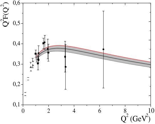
Figure 5: The $1\sigma$ region for the scaled pion FF $Q^{2}F_{\pi}(Q^{2})$. The data are taken from Refs. Beb (the circles) and Vol (the rectangles). In the $1\sigma$ analysis only the solid data points are used. For the central solid curve the input parameters are $b_{2}(\mu_{0}^{2})=0.2,\,\,b_{4}(\mu_{0}^{2})=0$.

The data points included into the fitting procedure are shown by the solid points. Here we take into account the data $Q^{2}\geq 1.18\,\,\rm{GeV}^{2}$ reported in Ref. Beb , and two new data points at $Q^{2}=1;\,\,1.6\,\,\rm{GeV}^{2}$ obtained by the $F_{\pi}$ collaboration Vol . From this analysis we extract the value of the input parameter $b_{2}(1\,\rm{GeV}^{2})$, in the case of the DA with one nonasymptotic term

$$b_{2}(1\ \rm{GeV}^{2})=0.2\pm 0.03.$$ (30)

For the pion DA with two nonasymptotic terms, we get

$$b_{2}(1\ \rm{GeV}^{2})=0.2\pm 0.03,\,\,b_{4}(1\ \rm{GeV}^{2})=-0.03\pm 0.06.$$ (31)

From Eqs. (30) and (31) it becomes evident that impact of $b_{2}(\mu_{0}^{2})$ on the numerical computations is more important than a role played by $b_{4}(\mu_{0}^{2})$. Our analysis does not exclude also DAs with two positive input parameters. But it is worth noting that in our consideration we have used the data Beb which were extracted indirectly from the pion electroproduction experiments through a model-dependent extrapolation to the pion pole. Moreover, the points $Q^{2}>2\ \rm{GeV}^{2}$ are imprecise suffering from the large errors and they are rather sparse. Correct and direct measurements of the form factor at $Q^{2}\geq 2\ \rm{GeV}^{2}$ will improve the performed analysis and allow one to put more strong constraints on the pion DAs.

In the region $1\ \rm{GeV}^{2}\leq$ $Q^{2}<10\ \rm{GeV}^{2}$, our prediction for the pion electromagnetic FF can be fitted to the following formula:

$$Q^{2}F_{\pi}(Q^{2})=(0.2227\pm 0.011)+\frac{0.5107\pm 0.0115}{Q^{2}}-\frac{0.4284\pm 0.0165}{Q^{4}},$$ (32)

where the uncertainties in the numerical coefficients are connected with the experimental errors.

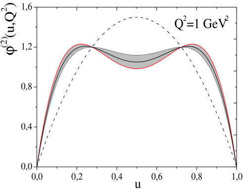
Figure 6: The pion leading twist DA extracted in this work. The scale $Q^{2}$ is fixed at $1\,\,\rm{GeV}^{2}$. For the central solid curve $b_{2}(\mu_{0}^{2})=0.2$. For comparison the asymptotic distribution amplitude is also shown (dashed curve).

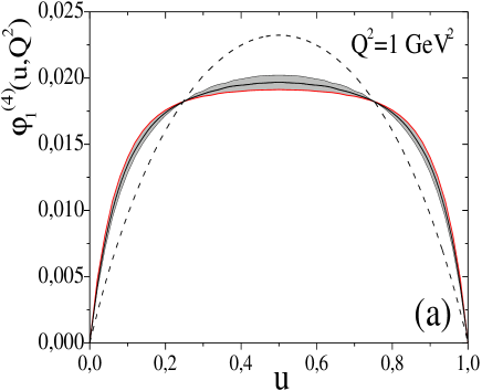
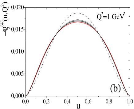
Figure 7: The two-particle twist-4 DAs $\varphi_{1}^{(4)}(u,Q^{2})$ (a), and $-\varphi_{2}^{(4)}(u,Q^{2})$ (b) obtained within the renormalon approach and using the constraint on the parameter $b_{2}(\mu_{0}^{2})$ (30). By dashed lines, for comparison, we plot the DAs obtained also within the renormalon approach, but using the pion asymptotic leading twist DA.

The pion twist-2 and two-particle twist-4 DAs calculated using the parameter (30) are shown in Figs. 6 and 7. The shaded areas in the figures are obtained varying the parameter $b_{2}(1\,\rm{GeV}^{2})$ within the allowed interval. The pion leading twist DA in the middle point $u_{0}=0.5$ takes the values

$$\varphi^{(2)}(0.5,1\ \rm{GeV}^{2})=1.05\mp 0.07,\ \varphi^{(2)}(0.5,10\ \rm{GeV}^{2})=1.18\mp 0.05.$$ (33)

This estimate is rather precise and does not contradict to the old Braun-Filyanov result,

$$\varphi^{(2)}(0.5)=1.2\pm 0.2,$$

from the second paper in Ref. BBK89 . The model DAs corresponding to Eq. (31) have the similar behavior and are not shown in the figures.

V Concluding remarks

In the present work we have used the renormalon approach to determine the pion twist-4 DAs. In this approach the higher twist DAs are expressed in terms of the leading twist DA unambiguously. This fact has allowed us to avoid expansion of the higher twist DAs over the conformal spin and, at the same time, to take into account higher conformal spin effects. Of course, the renormalon approach is not suitable to model higher spin effects in the leading twist DA. Nevertheless, it considerably restricts a possible form of the higher twist DAs.

The obtained model DAs have been employed for computation of the pion electromagnetic FF within the QCD LCSR method. For this purpose the correct expression for the twist-4 contribution to $F_{\pi}(Q^{2})$ has been used Bijnen and from comparison with the available experimental data the constraints on the input parameters $b_{2}(\mu_{0}^{2}),$ $b_{4}(\mu_{0}^{2})$ at $\mu_{0}^{2}=1\ \rm{GeV}^{2}$ have been deduced.

The pion twist-2 DA $\varphi_{\pi}(u,Q^{2})$ was an object of numerous investigations. It was modeled using the various theoretical schemes and exclusive processes (see, for example, Refs. CZ84 ; A01 ; pion ). The models found in the present work are close to ones predicted in Ref. A01 . In Ref. A01 the power-suppressed corrections to $F_{\pi}(Q^{2})$ were evaluated in the framework of the standard hard-scattering approximation and the running coupling method, which resulted in the Borel resummed FF $[Q^{2}F_{\pi}(Q^{2})]^{res}$ , whereas in the present paper we have computed the twist-4 contribution to $F_{\pi}(Q^{2})$ in the context of the LCSR method and the renormalon-inspired twist-4 DAs. The new contribution of this work is that the renormalon approach has allowed to put an upper bound on the twist-4 contribution to the sum rules and obtain estimates, for the first time, of the effects due to higher conformal spins. We have gotten similar values of the pion DA parameters compared to other studies, so the LCSR approach seems to be protected from large uncertainties coming from higher twist corrections.

Acknowledgments.

I am grateful to Prof. V. M. Braun for drawing to my attention this problem, reading the manuscript and for valuable comments. I would like also to thank Prof. J. P. Blaizot and ”European Centre for Theoretical Studies in Nuclear Physics and Related Areas” (ECT*) for hospitality in Trento, where this work was started and Prof. S. Randjbar-Daemi and members of the High Energy Section in the A. Salam ICTP, where it was completed.

References

• (1) A. V. Efremov and A. V. Radyushkin, Theor. Math. Phys. 42, 97 (1980) [Teor. Mat. Fiz. 42, 147 (1980)]; Phys. Lett. B 94, 245 (1980).
• (2) G. P. Lepage and S. J. Brodsky, Phys. Lett. B 87, 359 (1979); Phys. Rev. D 22, 2157 (1980).
• (3) V. M. Braun, G. P. Korchemsky and D. MΓΌller, Prog. Part. Nucl. Phys. 51, 311 (2003).
• (4) V. M. Braun and I. E. Filyanov, Z. Phys. CΒ 48, 239 (1990).
• (5) V. L. Chernyak and A. R. Zhitnitsky, Phys. Rep. 112, 173 (1984).
• (6) P. Ball, V. M. Braun, Y. Koike and K. Tanaka, Nucl. Phys. B529, 323 (1998).
• (7) P. Ball, V. M. Braun, Nucl. Phys. B543, 201 (1999).
• (8) P. Ball, J. High Energy Phys. 01, 010 (1999).
• (9) P. Ball, V. M. Braun and N. Kivel, Nucl. Phys. B649, 263 (2003).
• (10) J. R. Andersen, Phys. Lett. B 475, 141 (2000).
• (11) V. M. Braun, E. Gardi and S. Gottwald, Nucl. Phys. B685, 171 (2004).
• (12) I. I. Balitsky and V. M. Braun, Nucl. Phys. B311, 541 (1989).
• (13) V. M. Braun, S. E. Derkachov, G. P. Korchemsky and A. N. Manashov, Nucl. Phys. B553, 355 (1999).
• (14) V. M. Braun, G. P. Korchemsky and A. N. Manashov, Nucl. Phys. B603, 69 (2001).
• (15) V. L. Chernyak, A. R. Zhitnitsky and I. R. Zhitnitsky, Yad. Fiz. 38, 1074 (1983) [ Sov. J. Nucl. Phys. 38, 645 (1983)];
V. A. Novikov, M. A. Shifman, A. I. Vainstein, M. B. Voloshin, and V. I. Zakharov, Nucl. Phys. B237, 525 (1984).
• (16) I. I. Balitsky, V. M. Braun and A. V. Kolesnichenko, Nucl. Phys. B312, 509 (1989); V. M. Braun and I. E. Filyanov, Z. Phys. CΒ 44, 157 (1989); V. L. Chernyak and I. R. Zhitnitsky, Nucl. Phys. B345, 137 (1990).
• (17) V. Braun and I. Halperin, Phys. Lett. BΒ 328, 457 (1994).
• (18) V. M. Braun, A. Khodjamirian and M. Maul, Phys. Rev. DΒ 61, 073004 (2000).
• (19) J. Bijnens and A. Khodjamirian, Eur. Phys. J C 26, 67 (2002).
• (20) S. S. Agaev, Phys. Rev. DΒ 69, 094010 (2004).
• (21) S. S. Agaev, Phys. Rev. DΒ 64, 014007 (2001); S. S. Agaev and N. G. Stefanis, Phys. Rev. DΒ 70, 054020 (2004).
• (22) P. Gosdzinsky and N. Kivel, Nucl. Phys. B521, 274 (1998).
• (23) M. A. Shifman, A. I. Vainstein and V. I. Zakharov, Nucl. Phys. B147, 385; 448 (1979).
• (24) C. J. Bebek et al., Phys. Rev. DΒ 17, 1693 (1978).
• (25) J. Volmer et al., Phys. Rev. Lett. 86, 1713 (2001).
• (26) G. R. Farrar, K. Huleihel and H. Zhang, Nucl. Phys. B349, 655 (1991); A. Schmedding and O. Yakovlev, Phys. Rev. D 62, 116002 (2000); A. P. Bakulev, S. V. Mikhailov and N. G. Stefanis, Phys. Rev. D 67, 074012 (2003).