$J/\Psi$ and $\Psi^{\prime}$ Polarizations in Polarized Proton-Proton
Collisions at the RHIC

Abstract

We study inclusive heavy quarkonium production with definite polarizations in polarized proton-proton collisions using the non-relativistic QCD color-octet mechanism. We present results for rapidity distributions of cross sections and spin asymmetries for the production of $J/\psi$ and $\psi^{\prime}$ with specific polarizations in polarized p-p collisions at $\sqrt{s}$ = 200 GeV and 500 GeV at the RHIC within the PHENIX detector acceptance range.

I Introduction

The relativistic heavy ion collider (RHIC) at BNL is a unique facility which collides two heavy ions at $\sqrt{s}$ = 200 GeV to study the production of a quark-gluon plasma qgp and two polarized protons to study the parton spin structure of the proton spin . Measurements of heavy probes such as $J/\psi$ production and Drell-Yan production are useful tools to study the quark-gluon plasma in heavy ion collisions and to extract the polarized gluon distribution functions inside the proton in polarized p-p collisions phenix ; QWGBrambilla . Understanding the correct production mechanisms for these processes is important. Heavy quarkonium production can be described via the non-relativistic QCD (NRQCD) color-octet mechanism bodwin ; nayak .

In NRQCD the energy eigenstates of heavy quarkonium bound states $|H>$ are labelled by the quantum numbers $J^{PC}$, with an additional superscript to give the color; (1) for singlet and (8) for octet. When the Fock states are analysed then the dominant component in S-wave orthoquarkonium is the pure quark-antiquark state $|Q\bar{Q}[^{3}S^{(1)}_{1}]>$. A state with dynamical gluons, such as $|Q\bar{Q}[^{3}P^{(8)}_{J}]g>$ does contribute but only with a probability of order $v^{2}$, where $v$ is the typical velocity of the non-relativistic heavy quark (and antiquark). The other states, such as $|Q\bar{Q}[^{3}S^{(1,8)}_{1}]gg>$, $|Q\bar{Q}[^{1}S^{(8)}_{0}]g>$ and $|Q\bar{Q}[^{3}D^{(1,8)}_{J}]gg>$ contribute to the probability in even higher orders in $v$ (see later). Correspondingly the dominant states in P-wave orthoquarkonia are the states $|Q\bar{Q}[^{3}P^{(1)}_{J}]>$, and the states with dynamical gluons such as $|Q\bar{Q}[^{3}S^{(8)}_{1}]g>$ contribute with a probability of order $v^{2}$. After a $Q\bar{Q}$ is formed in a color octet state it may emit a soft gluon to transform into the singlet state $|Q\bar{Q}[^{3}P^{(1)}_{J}]>$ and then become a $J/\psi$ state by photon decay. The $Q\bar{Q}$ pair in a color octet state can also emit two long wavelength gluons and then become a $J/\psi$ state. All these low energy interactions are negligible and the non-perturbative matrix elements, labelled by the above quantum numbers, can be fitted from experiments or can be determined from lattice field theory calculations.

Using the NRQCD color octet mechanism heavy quarkonia production rates have been calculated for the p-$\bar{\rm p}$ Tevatron collider CDFoctet ; CL , for the e-p HERA collider HERAoctet , for the e⁺-e^- LEP collider LEPoctet and for fixed target experiments fixedtargetoctet . Also the recent PHENIX data for $J/\psi$ production in unpolarized p-p collisions can be explained by this same mechanism cooper .

The RHIC offers a wide variety of measurements with respect to $J/\psi$ production. They involve $J/\psi$ production (with and without definite polarizations), in unpolarized p-p, d-Au, Cu-Cu and Au-Au collisions and in polarized p-p collisions. Since the maximum transverse momentum of heavy quarkonium that can be measured at the RHIC is around 10 GeV/c, the parton fragmentation contribution to heavy quarkonium production will be very small and we will neglect it in our study. The main contributions to heavy quarkonium production at the RHIC are the parton fusion processes cooper ; pol .

The inclusive heavy quarkonium production cross section (summed over quarkonium polarization states) in unpolarized and polarized partonic collisions were calculated in CL ; fm and pol ; gm respectively. Heavy quarkonium production cross sections with definite polarizations in unpolarized partonic collisions were calculated in braaten ; CDFpolarization . In this paper we will study the inclusive rapidity distributions for heavy quarkonium production with specific polarizations in polarized p-p collisions. We will evaluate the partonic level cross sections for the processes $q\bar{q},~{}gg~{}\rightarrow~{}J/\psi(\lambda)(\psi^{\prime}(\lambda))$ in polarized p-p collisions where $\lambda$ is the helicity (polarization) of the heavy quarkonium state. This study should be regarded as a preliminary analysis of the leading order (LO) contributions to charmonium production in specific polarization states. The factorization ansatz, which separates the short-distance coefficient functions, calculable in perturbative QCD, from the long distance matrix elements, which are fitted to data, is only proved if the charmonium state is produced at a large transverse momentum nayak . Our LO analysis considers only charmonium production in the forward direction at a finite rapidity. It will be followed later by a next-to-leading (NLO) calculation where additional quark and/or gluon radiation is produced in the final state so that the charmonium state does have a finite transverse momentum. The reason we need these results is that the PHENIX collaboration at the RHIC will measure $J/\psi$ and $\psi^{\prime}$ production with definite polarizations in polarized p-p collisions at $\sqrt{s}$ = 200 GeV and 500 GeV phenix . Since polarized heavy quarkonium production at the Tevatron energy scale expt is not explained by the NRQCD color-octet mechanism CDFpolarization it will be useful to compare our results for $J/\psi$ and $\psi^{\prime}$ polarizations with the future data at the RHIC. The study of polarized heavy quarkonium production in polarized p-p collisions at the RHIC is also unique in the sense that it probes the spin transfer processes in perturbative QCD (pQCD). Note that decays from higher quarkonium states to the $J/\psi$ are ignored. We only consider direct production.

The spin projection method is used to evaluate the inclusive cross section for heavy quarkonium production (summed over polarization states) in parton fusion processes CL . However, the cross section for heavy quarkonium production with a specific polarization in the final state can involve additional matrix elements that do not contribute when the polarization is summed. This includes interference terms between partonic processes that produce heavy quark-antiquark pairs with different total angular momenta. Such interference terms cancel upon summing over polarizations. These interference terms can be calculated by using the helicity decomposition method braaten . Hence we will use the helicity decomposition method to calculate the square of the matrix elements for heavy quarkonium production with definite helicity in polarized partonic collisions. Using these results we will compute the rapidity distributions of the cross sections and spin asymmetries of heavy quarkonium production with definite helicity states in polarized p-p collisions at RHIC at $\sqrt{s}$ = 200 GeV and 500 GeV within the PHENIX detector acceptance ranges.

The paper is organized as follows. In section II we derive the partonic level cross sections for heavy quarkonium production with definite polarizations in polarized q-$\bar{\rm q}$ and g-g parton fusion processes using the helicity decomposition method within the NRQCD color-octet mechanism. In section III we present the results for the differential rapidity distributions and spin asymmetries for the $J/\psi(\lambda)$ and $\psi^{\prime}(\lambda)$ in the PHENIX detector acceptance range in polarized p-p collisions at $\sqrt{s}$ = 200 GeV and 500 GeV. We then discuss these results and give our conclusions.

II Inclusive Heavy Quarkonium Production with Definite
Helicities in Polarized Partonic Collisions

In this section we will use the NRQCD color-octet mechanism and derive the square of the matrix element for inclusive heavy quarkonium production with definite helicities in polarized partonic fusion processes. We will consider the (polarized) partonic fusion processes $q\bar{q}~{}\rightarrow~{}H(\lambda)$ and $gg~{}\rightarrow~{}H(\lambda)$ where $\lambda$ is the helicity of the produced heavy quarkonium state $H$. We will use the helicity decomposition method braaten within the NRQCD color-octet mechanism to calculate these processes where both initial and final state particles are polarized.

II.1 The $q\bar{q}$ fusion process

The production of a heavy charmonium state with helicity $\lambda$, where $\lambda=0,\pm 1$ correspond to longitudinal and transverse polarization states respectively, begins with the calculation of the production of a heavy quark anti-quark pair. The matrix element for the light quark-antiquark ($q\bar{q}$) fusion process $q(k_{1})+\bar{q}(k_{2})\rightarrow Q(p_{1})+\bar{Q}(p_{2})$ producing a heavy quark-antiquark ($Q\bar{Q}$) pair is given by

$$M_{q\bar{q}\rightarrow Q\bar{Q}}~{}=~{}\frac{g^{2}}{P^{2}}~{}\bar{v}(k_{2})\gamma_{\mu}T^{a}u(k_{1})\,\bar{u}(p_{1})\gamma^{\mu}T^{a}v(p_{2})\,,$$ (1)

where $P^{\mu}~{}=~{}p_{1}^{\mu}~{}+~{}p_{2}^{\mu}~{}=~{}k_{1}^{\mu}~{}+~{}k_{2}^{\mu}$ and $p_{1}^{\mu}=P^{\mu}/2+L^{\mu}_{j}q^{j}$ and $p_{2}^{\mu}=P^{\mu}/2-L^{\mu}_{j}q^{j}$. Here $P^{\mu}$ is the CM momentum of the pair and $q^{i}$ is their relative momentum in the CM frame. The latter vector does not have any time component so $i=1,2,3$ only. $L^{\mu}_{j}$ is the boost matrix defined in braaten with both Lorentz and three vector indices. In terms of non-relativistic heavy quark Pauli spinors ($\xi$ and $\eta$) we obtain (up to terms linear in $q$):

$$|M_{q\bar{q}\rightarrow Q\bar{Q}}|^{2}~{}=~{}\frac{g^{4}}{4m^{2}}~{}{\eta^{\prime}}^{\dagger}\sigma^{i}T^{a}{\xi^{\prime}}\,L^{\mu}_{i}\,\bar{u}(k_{1})\gamma_{\mu}T^{a}v(k_{2})\,\bar{v}(k_{2})\gamma_{\nu}T^{b}u(k_{1})\,L^{\nu}_{j}\,{\xi}^{\dagger}\sigma^{j}T^{b}{\eta}\,,$$ (2)

where $m$ is the mass of the heavy quark. For massless incoming quarks and antiquarks we have

$$u(k_{1})\bar{u}(k_{1})~{}=~{}\frac{1}{2}~{}(1+h_{1}\gamma_{5})~{}\gamma_{\mu}k_{1}^{\mu}$$

$$~{}v(k_{2})\bar{v}(k_{2})~{}=~{}\frac{1}{2}~{}(1-h_{2}\gamma_{5})~{}\gamma_{\mu}k_{2}^{\mu}\,.$$ (3)

The polarized partonic matrix element squared involves the helicity combination $(+,+)-(+,-)$ with $+,-$ denoting the helicities $h_{1}$, $h_{2}$ of the incoming partons. Then from eq. (2) we find

$$\Delta~{}|M_{q\bar{q}\rightarrow Q\bar{Q}}|^{2}~{}=~{}\frac{g^{4}}{4m^{2}}~{}{\eta^{\prime}}^{\dagger}\sigma^{i}T^{a}{\xi^{\prime}}\,{\xi}^{\dagger}\sigma^{j}T^{a}{\eta}\,~{}[2m^{2}n_{i}n_{j}~{}-~{}\delta_{ij}(k_{1}\cdot k_{2})]\,,$$ (4)

using $(k_{2}\cdot L)_{i}=-(k_{1}\cdot L)_{i}~{}=~{}m~{}n_{i}$. Here $n_{i},n_{j}$ are the components of unit three-vectors ${\bf n}_{1},{\bf n}_{2}$ which specify the polarizations of the heavy quarks and heavy antiquarks respectively in the charmonium bound state. Their $z$-components are usually chosen along the beam direction. In a frame where $\bf{P},\bf{k_{1}}$, and $\bf{k_{2}}$ are collinear, they are also collinear with the third components of ${\bf n}_{1},{\bf n}_{2}$. Taking the leading order term in an expansion in $q$ so that $P^{2}=4m^{2}$ we obtain

$$\Delta~{}|M_{q\bar{q}\rightarrow Q\bar{Q}}|^{2}~{}=~{}\frac{g^{4}}{4}~{}[n_{i}n_{j}-\delta_{ij}]~{}{\eta^{\prime}}^{\dagger}\sigma^{i}T^{a}{\xi^{\prime}}\,{\xi}^{\dagger}\sigma^{j}T^{a}{\eta}\,.$$ (5)

Averaging over the initial color (by dividing by 9), we therefore get

$$\Delta~{}|M_{q\bar{q}\rightarrow Q\bar{Q}}|^{2}~{}=~{}\frac{4\pi^{2}\alpha_{s}^{2}}{9}~{}[n_{i}n_{j}-\delta_{ij}]~{}{\eta^{\prime}}^{\dagger}\sigma^{i}T^{a}{\xi^{\prime}}{\xi}^{\dagger}\sigma^{j}T^{a}{\eta}\,.$$ (6)

The two-component spinor factors can be identified with various heavy quarkonium bound states $H(\lambda)$ with different quantum numbers as follows, (see Appendix B in braaten )

$$~{}4m^{2}~{}\eta^{\prime\dagger}\xi^{\prime}\,\xi^{\dagger}\eta~{}\equiv~{}<\chi^{\dagger}\psi\,P_{H(\lambda)}\,~{}\psi^{\dagger}\chi>~{}=~{}\frac{4}{3}m<{\cal O}^{H}_{1}(^{1}S_{0})>\,,$$

$$~{}4m^{2}~{}\eta^{\prime\dagger}T^{a}\xi^{\prime}\,\xi^{\dagger}T^{a}\eta~{}\equiv~{}<\chi^{\dagger}T^{a}\psi\,P_{H(\lambda)}\,~{}\psi^{\dagger}T^{a}\chi>~{}=~{}\frac{4}{3}m<{\cal O}^{H}_{8}(^{1}S_{0})>\,,$$

$$~{}4m^{2}~{}\eta^{\prime\dagger}\sigma^{i}\xi^{\prime}\,\xi^{\dagger}\sigma^{j}\eta~{}\equiv~{}<\chi^{\dagger}\sigma^{i}\psi\,P_{H(\lambda)}\,~{}\psi^{\dagger}\sigma^{j}\chi>~{}=~{}\frac{4}{3}U^{\dagger}_{\lambda i}U_{j\lambda}m<{\cal O}^{H}_{1}(^{3}S_{1})>\,,$$

$$~{}4m^{2}~{}\eta^{\prime\dagger}\sigma^{i}T^{a}\xi^{\prime}\,\xi^{\dagger}\sigma^{j}T^{a}\eta~{}\equiv~{}<\chi^{\dagger}\sigma^{i}T^{a}\psi\,P_{H(\lambda)}\,~{}\psi^{\dagger}\sigma^{j}T^{a}\chi>~{}=~{}\frac{4}{3}U^{\dagger}_{\lambda i}U_{j\lambda}m<{\cal O}^{H}_{8}(^{3}S_{1})>\,,$$

$$~{}4m^{2}~{}q^{n}{q^{m}}\eta^{\prime\dagger}\sigma^{i}\xi^{\prime}\,\xi^{\dagger}\sigma^{j}\eta~{}\equiv~{}<\chi^{\dagger}(-\frac{i}{2}D^{m})\sigma^{i}\psi\,P_{H(\lambda)}\,~{}\psi^{\dagger}(-\frac{i}{2}D^{n})\sigma^{j}\chi>$$

$$~{}=~{}4U^{\dagger}_{\lambda i}\,U_{j\lambda}\delta^{mn}m<{\cal O}^{H}_{1}(^{3}P_{0})>\,,$$

$$~{}4m^{2}~{}q^{n}{q^{m}}\eta^{\prime\dagger}\sigma^{i}T^{a}\xi^{\prime}\xi^{\dagger}\sigma^{j}T^{a}\eta~{}\equiv~{}<\chi^{\dagger}(-\frac{i}{2}D^{m})\sigma^{i}T^{a}\psi\,P_{H(\lambda)}~{}\psi^{\dagger}(-\frac{i}{2}D^{n})\sigma^{j}T^{a}\chi>$$

$$~{}=~{}4U^{\dagger}_{\lambda i}\,U_{j\lambda}\delta^{mn}m<{\cal O}^{H}_{8}(^{3}P_{0})>\,.$$ (7)

The helicity index $\lambda$ is a vector index in the spherical basis. The spherical basis states and cartesian basis states are related by a unitary transformation matrix $U_{\lambda i}$ which satisfies the relation

$$\sum_{i}U_{\lambda i}U^{\dagger}_{i\lambda}~{}=~{}1$$

$$\sum_{i}U_{\lambda i}n^{i}=\delta_{\lambda 0}\,,$$ (8)

where $n^{i}$ is along the z-direction. Using the above relations we finally obtain

$$\Delta|M_{q\bar{q}\rightarrow H(\lambda)}|^{2}~{}=~{}-\frac{4\pi^{2}\alpha_{s}^{2}}{27}~{}[1-\delta_{\lambda 0}]~{}<{\cal{O}}^{H}_{8}(^{3}S_{1})>\,.$$ (9)

The polarized quark-antiquark fusion process cross section is given by

$$\Delta\sigma_{q\bar{q}\rightarrow H(\lambda)}~{}=~{}-\delta(\hat{s}-4m^{2})~{}\frac{\pi^{3}\alpha_{s}^{2}}{27m^{3}}~{}[1-\delta_{\lambda 0}]~{}<{\cal{O}}^{H}_{8}(^{3}S_{1})>\,,$$ (10)

and therefore vanishes for $\lambda=0$.

II.2 The gg fusion process

The matrix element for the gluon fusion process $g(k_{1})+g(k_{2})\rightarrow Q(p_{1})+\bar{Q}(p_{2})$ after including s, t, and u channel Feynman diagrams is given by

$$M_{gg\rightarrow Q\bar{Q}}~{}=~{}-g^{2}~{}\epsilon^{a}_{\mu}(k_{1})\epsilon^{*b}_{\nu}(k_{2})~{}[(\frac{1}{6}\delta^{ab}~{}+~{}\frac{1}{2}d^{abc}T^{c})~{}S^{\mu\nu}~{}+~{}\frac{i}{2}f^{abc}T^{c}~{}F^{\mu\nu}]\,,$$ (11)

where

$$S^{\mu\nu}~{}=~{}\bar{u}(p_{1})[\frac{\gamma^{\mu}~{}({{p}\!\!\!/}_{1}-{{k}\!\!\!/}_{1}+m)~{}\gamma^{\nu}}{2p_{1}\cdot k_{1}}~{}+~{}\frac{\gamma^{\nu}~{}({{p}\!\!\!/}_{1}-{{k}\!\!\!/}_{2}+m)~{}\gamma^{\mu}}{2p_{1}\cdot k_{2}}]\,v(p_{2})$$ (12)

and

$$F^{\mu\nu}~{}=~{}\bar{u}(p_{1})[\frac{\gamma^{\mu}~{}({{p}\!\!\!/}_{1}-{{k}\!\!\!/}_{1}+m)~{}\gamma^{\nu}}{2p_{1}\cdot k_{1}}~{}-~{}\frac{\gamma^{\nu}~{}({{p}\!\!\!/}_{1}-{{k}\!\!\!/}_{2}+m)~{}\gamma^{\mu}}{2p_{1}\cdot k_{2}}$$

$$~{}+~{}\frac{2}{P^{2}}~{}V^{\mu\nu\lambda}(k_{1},k_{2},-k_{1}-k_{2})~{}\gamma_{\lambda}]v(p_{2})\,.$$ (13)

The three gluon vertex is denoted by $V^{\mu\nu\lambda}(k_{1},k_{2},k_{3})~{}=~{}[(k_{1}-k_{2})^{\lambda}g^{\mu\nu}~{}+~{}(k_{2}-k_{3})^{\mu}g^{\nu\lambda}~{}+~{}(k_{3}-k_{1})^{\nu}g^{\lambda\mu}]$. Using various identities among the spinors and boost matrices from the appendix A of braaten and after performing a considerable amount of algebra we find

$$\bar{u}(p_{1})[\frac{\gamma^{\mu}~{}{{k}\!\!\!/}_{1}~{}\gamma^{\nu}}{2p_{1}\cdot k_{1}}~{}+~{}\frac{\gamma^{\nu}{{k}\!\!\!/}_{2}~{}\gamma^{\mu}}{2p_{1}\cdot k_{2}}]v(p_{2})~{}=~{}\frac{i}{2m^{2}}(k_{1}-k_{2})_{\lambda}\epsilon^{\rho\mu\nu\lambda}P_{\rho}\xi^{\dagger}\eta$$

$$~{}+~{}\frac{(L\cdot k_{1})_{n}}{m^{3}}~{}[P^{\nu}L^{\mu}_{j}-P^{\mu}L^{\nu}_{j}+2g^{\mu\nu}(L\cdot k_{1})_{j}-(k_{1}-k_{2})^{\mu}L^{\nu}_{j}-(k_{1}-k_{2})^{\nu}L^{\mu}_{j}]~{}q^{n}\xi^{\dagger}\sigma^{j}\eta$$

$$~{}+~{}\frac{(L\cdot k_{1})_{j}}{m^{3}}~{}[P^{\mu}L^{\nu}_{n}-P^{\nu}L^{\mu}_{n}]~{}q^{n}\xi^{\dagger}\sigma^{j}\eta~{}+~{}\frac{1}{m}~{}[P^{\mu}L^{\nu}_{j}-P^{\nu}L^{\mu}_{j}]~{}\xi^{\dagger}\sigma^{j}\eta\,,$$ (14)

and

$$\bar{u}(p_{1})[\frac{\gamma^{\mu}~{}{{k}\!\!\!/}_{1}~{}\gamma^{\nu}}{2p_{1}\cdot k_{1}}~{}-~{}\frac{\gamma^{\nu}{{k}\!\!\!/}_{2}~{}\gamma^{\mu}}{2p_{1}\cdot k_{2}}]v(p_{2})~{}=~{}\frac{(L\cdot k_{1})_{n}}{2m^{4}}(k_{1}-k_{2})_{\lambda}\epsilon^{\rho\mu\nu\lambda}P_{\rho}q^{n}\xi^{\dagger}\eta$$

$$~{}-~{}\frac{(L\cdot k_{1})_{n}}{m^{3}}~{}[P^{\nu}L^{\mu}_{j}+P^{\mu}L^{\nu}_{j}]~{}q^{n}\xi^{\dagger}\sigma^{j}\eta$$

$$-\frac{1}{m}~{}[2g^{\mu\nu}(L\cdot k_{1})_{j}-(k_{1}-k_{2})^{\mu}L^{\nu}_{j}-(k_{1}-k_{2})^{\nu}L^{\mu}_{j}]~{}\xi^{\dagger}\sigma^{j}\eta$$

$$~{}+~{}\frac{2}{m}~{}[L^{\mu}_{n}L^{\nu}_{j}-L^{\nu}_{n}L^{\mu}_{j}]~{}q^{n}\xi^{\dagger}\sigma^{j}\eta\,.$$ (15)

Hence

$$S^{\mu\nu}~{}=~{}\frac{i}{2m^{2}}(k_{1}-k_{2})_{\lambda}\epsilon^{\rho\mu\nu\lambda}P_{\rho}\xi^{\dagger}\eta~{}+~{}[\frac{(L\cdot k_{1})_{j}}{m^{3}}~{}(P^{\nu}L^{\mu}_{n}-P^{\mu}L^{\nu}_{n}-2g^{\mu\nu}(L\cdot k_{1})_{n})$$

$$~{}+~{}\frac{2}{m}~{}[L^{\mu}_{n}L^{\nu}_{j}+L^{\nu}_{n}L^{\mu}_{j}]+\frac{1}{m^{3}}(L\cdot k_{1})_{n}[(k_{1}-k_{2})^{\mu}L^{\nu}_{j}+(k_{1}-k_{2})^{\nu}L^{\mu}_{j}]]~{}q^{n}\xi^{\dagger}\sigma^{j}\eta\,,$$ (16)

which is symmetric under $k_{1}\leftrightarrow k_{2}$, $\mu\leftrightarrow\nu$ because $(k_{1}\cdot L)_{i}=-(k_{2}\cdot L)_{i}$, and

$$F^{\mu\nu}~{}=~{}\frac{i(L\cdot k_{1})_{n}}{2m^{4}}(k_{1}-k_{2})_{\lambda}\epsilon^{\rho\mu\nu\lambda}P_{\rho}q^{n}\xi^{\dagger}\eta+[k_{2}^{\nu}L^{\mu}_{j}-k_{1}^{\mu}L^{\nu}_{j}]~{}\xi^{\dagger}\sigma^{j}\eta\,,$$ (17)

which is antisymmetric under the interchanges above. For an incoming gluon with a helicity $\lambda_{1}$ the square of gluon polarization vector can be written as sivers

$$\epsilon^{a}_{\mu}(k_{1},\lambda_{1})\epsilon^{*b}_{\nu}(k_{1},\lambda_{1})~{}=~{}\frac{1}{2}~{}\delta^{ab}~{}[-g_{\mu\nu}~{}+\frac{k_{1\mu}k_{2\nu}+k_{2\mu}k_{1\nu}}{k_{1}\cdot k_{2}}-i\lambda_{1}~{}\epsilon_{\mu\nu\rho\delta}\frac{k_{1}^{\rho}k_{2}^{\delta}}{k_{1}\cdot k_{2}}]\,,$$ (18)

with a similar result for the square of the second polarization vector $\epsilon^{a}_{\mu}(k_{2},\lambda_{2})\epsilon^{*b}_{\nu}(k_{2},\lambda_{2})$. Using the relation

$$\epsilon_{\mu\mu^{\prime}\alpha\beta}~{}k_{1}^{\alpha}k_{2}^{\beta}~{}=~{}2m^{2}\epsilon^{ijk}n_{k}L^{\mu}_{i}L^{\nu}_{j}\,,$$ (19)

from appendix A of braaten and choosing longitudinally polarized gluons we find that

$$~{}\Delta|M_{gg\rightarrow Q\bar{Q}}|^{2}~{}=~{}-\frac{g^{4}}{4}~{}\epsilon^{pqr}\epsilon^{p^{\prime}q^{\prime}r^{\prime}}n_{r}n_{r^{\prime}}$$

$$~{}\times[S^{ab}S^{*ab}L_{\mu p}L_{\nu p^{\prime}}S^{\mu\nu}L_{\mu^{\prime}q}L_{\nu^{\prime}q^{\prime}}S^{*\mu^{\prime}\nu^{\prime}}+F^{ab}F^{*ab}L_{\mu p}L_{\nu p^{\prime}}F^{\mu\nu}L_{\mu^{\prime}q}L_{\nu^{\prime}q^{\prime}}F^{*\mu^{\prime}\nu^{\prime}}]\,,$$ (20)

where

$$S^{ab}~{}=~{}\frac{1}{6}\delta^{ab}~{}+~{}\frac{1}{2}d^{abc}T^{c}~{}~{}~{}~{}~{}~{}~{}{\rm and}~{}~{}~{}~{}~{}~{}~{}~{}~{}F^{ab}~{}=~{}\frac{i}{2}f^{abc}T^{c}\,.$$ (21)

The cross terms between $S$ and $F$ vanish because

$$S^{ab}F^{*ab}~{}=~{}0~{}=~{}S^{*ab}F^{ab}\,,$$ (22)

due to their symmetry properties. Using various properties of the $L^{\mu}_{i}$ matrices from appendix A of braaten and performing some lengthy algebra we finally obtain, after averaging over the initial color (by dividing by 64),

$$\Delta|M_{gg\rightarrow Q\bar{Q}}|^{2}~{}=~{}-\frac{\pi^{2}\alpha_{s}^{2}}{9}~{}[\eta^{\prime\dagger}\xi^{\prime}\xi^{\dagger}\eta+\frac{1}{m^{2}}[(n\cdot q)n_{j}q^{\prime}_{j^{\prime}}+(n\cdot q^{\prime})n_{j^{\prime}}q_{j}-\frac{3}{2}(n\cdot q)(n\cdot q^{\prime})n_{j}n_{j^{\prime}}$$

$$-(n\times q^{\prime})_{j}(n\times q)_{j^{\prime}}]\eta^{\prime\dagger}\sigma^{j^{\prime}}\xi^{\prime}\xi^{\dagger}\sigma^{j}\eta+\frac{15}{8}\eta^{\prime\dagger}T^{a}\xi^{\prime}\xi^{\dagger}T^{a}\eta+\frac{15}{8m^{2}}[(n\cdot q)n_{j}q^{\prime}_{j^{\prime}}+(n\cdot q^{\prime})n_{j^{\prime}}q_{j}$$

$$-\frac{3}{2}(n\cdot q)(n\cdot q^{\prime})n_{j}n_{j^{\prime}}-(n\times q^{\prime})_{j}(n\times q)_{j^{\prime}}]\eta^{\prime\dagger}\sigma^{j^{\prime}}T^{a}\xi^{\prime}\xi^{\dagger}\sigma^{j}T^{a}\eta$$

$$+\frac{27}{8m^{2}}~{}(n\cdot q)(n\cdot q^{\prime})\eta^{\prime\dagger}T^{a}\xi^{\prime}\xi^{\dagger}T^{a}\eta]\,.$$ (23)

After identifying the different bound states as given in eq. (7) and then using eq. (8) we obtain

$$\Delta|M_{gg\rightarrow H(\lambda)}|^{2}~{}=~{}-\frac{\pi^{2}\alpha_{s}^{2}}{27}~{}[<{\cal O}^{H}_{1}(^{1}S_{0})>~{}+~{}\frac{15}{8}<{\cal O}^{H}_{8}(^{1}S_{0})>$$

$$+\frac{3}{m^{2}}(\frac{1}{2}\delta_{\lambda 0}-1)[<{\cal O}^{H}_{1}(^{3}P_{0})>+\frac{15}{8}<{\cal O}^{H}_{8}(^{3}P_{0})>]~{}+~{}\frac{81}{8m^{2}}<{\cal O}^{H}_{8}(^{1}P_{1})>]\,.$$ (24)

Hence the partonic level inclusive cross sections for heavy quarkonium production with definite helicities $\lambda$ in polarized g-g collisions are given by

$$\Delta\sigma_{gg\rightarrow H(\lambda)}~{}=~{}-\delta(\hat{s}-4m^{2})~{}\frac{\pi^{3}\alpha_{s}^{2}}{108m^{3}}~{}[<{\cal O}^{H}_{1}(^{1}S_{0})>~{}+~{}\frac{15}{8}<{\cal O}^{H}_{8}(^{1}S_{0})>$$

$$+\frac{3}{m^{2}}(\frac{1}{2}\delta_{\lambda 0}-1)~{}[<{\cal O}^{H}_{1}(^{3}P_{0})>~{}+~{}\frac{15}{8}<{\cal O}^{H}_{8}(^{3}P_{0})>]~{}+~{}\frac{81}{8m^{2}}<{\cal O}^{H}_{8}(^{1}P_{1})>]\,.$$ (25)

III Results and Discussion

Using the formulae derived above we compute the LO rapidity distributions and spin asymmetries for the heavy charmonium systems $J/\psi$ and $\psi^{\prime}$ in longitudinally polarized proton-proton collisions at RHIC. This provides interesting information on the polarization state of these heavy charmonium states. In terms of the heavy quark relative velocity $v$, the non-perturbative matrix elements for ${\cal O}_{8}(^{3}P_{J})$ and ${\cal O}_{8}(^{3}S_{1})$ production scale like $v^{7}$ and for ${\cal O}_{8}(^{1}S_{0})$ production scales like $v^{6}$ whereas those for ${\cal O}_{8}(^{1}P_{1})$, ${\cal O}_{1}(^{1}S_{0})$, production scale like $v^{10}$ and ${\cal O}_{1}(^{3}P_{J})$ production scale like $v^{11}$ braaten ; bodwin . Hence we will not include the latter contributions as they are expected to be small. In particular this means that contributions from processes in which the $Q\bar{Q}$ pair is produced in color-singlet states are not included. Folding eqs. (10), (25) with parton densities we find the following cross sections in longitudinally polarized proton-proton collisions

$$\Delta\sigma_{(pp\rightarrow J/\psi(\lambda)(\psi^{\prime}(\lambda)))}~{}=~{}\frac{\pi^{3}\alpha_{s}^{2}}{27sm^{3}}~{}\int_{4m^{2}/s}^{1}\frac{dx_{1}}{x_{1}}~{}[\Delta f_{q}(x_{1},2m)~{}\Delta f_{\bar{q}}(\frac{4m^{2}}{x_{1}s},2m)$$

$$~{}\times~{}(\delta_{\lambda 0}-1)\,<{\cal{O}}^{J/\psi(\psi^{\prime})}_{8}(^{3}S_{1})>~{}+~{}\frac{15}{32}~{}\Delta f_{g}(x_{1},2m)~{}\Delta f_{g}(\frac{4m^{2}}{x_{1}s},2m)$$

$$~{}\times~{}[\frac{9}{m^{2}}(1-\frac{1}{2}\delta_{\lambda 0})<{\cal O}^{J/\psi(\psi^{\prime})}_{8}(^{3}P_{0})>~{}-~{}<{\cal O}^{J/\psi(\psi^{\prime})}_{8}(^{1}S_{0})>]]\,,$$ (26)

where $\Delta f(x,Q)(\Delta g(x,Q))$ denote the polarized quark (gluon) distribution functions inside the proton at the scale $Q$. The corresponding production cross sections for unpolarized proton-proton collisions are braaten :

$$\sigma_{(pp\rightarrow J/\psi(\lambda)(\psi^{\prime}(\lambda)))}~{}=~{}\frac{\pi^{3}\alpha_{s}^{2}}{27sm^{3}}~{}\int_{4m^{2}/s}^{1}\frac{dx_{1}}{x_{1}}~{}[f_{q}(x_{1},2m)~{}f_{\bar{q}}(\frac{4m^{2}}{x_{1}s},2m)$$

$$~{}\times~{}(1-\delta_{\lambda 0})~{}<{\cal{O}}^{J/\psi(\psi^{\prime})}_{8}(^{3}S_{1})>~{}+~{}\frac{15}{32}~{}f_{g}(x_{1},2m)~{}f_{g}(\frac{4m^{2}}{x_{1}s},2m)$$

$$~{}\times~{}[\frac{9}{m^{2}}(1-\frac{2}{3}\delta_{\lambda 0})<{\cal O}^{J/\psi(\psi^{\prime})}_{8}(^{3}P_{0})>~{}+~{}<{\cal O}^{J/\psi(\psi^{\prime})}_{8}(^{1}S_{0})>]]\,.$$ (27)

The spin asymmetry $A_{LL}(\lambda)$ is given by the ratio of the above cross sections

$$A_{LL}(\lambda)~{}=~{}\frac{d\Delta\sigma(\lambda)}{d\sigma(\lambda)}\,.$$ (28)

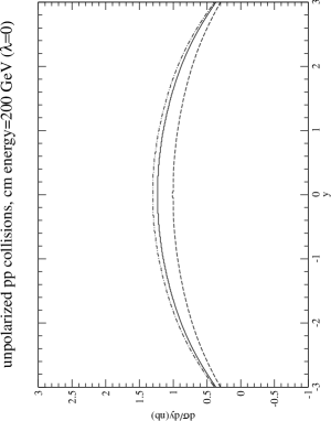
Figure 1: Differential rapidity distributions for $J/\psi$ production at $\sqrt{s}$ = 200 GeV. The solid, dashed and dot-dashed lines, each to be multiplied by a scale factor of 200, are for unpolarized p-p collisions with $J/\psi$ helicities $\lambda$ = 0 in scenarios 1, 2 and 3 respectively.

We begin with a discussion of the rapidity distribution for $J/\psi$ production. Color octet contributions have been obtained from an analysis of charmonium transverse momenta differential cross section data from the Fermilab Tevatron, see BK and CL . In particular central values are known for $<{\cal{O}}^{J/\psi}_{8}(^{3}S_{1})>$ and the combination

$$M^{J/\psi}(^{1}S_{0}^{(8)},{}^{3}P_{0}^{(8)})=<{\cal{O}}^{J/\psi}_{8}(^{1}S_{0})>+3.5<{\cal{O}}^{J/\psi}_{8}(^{3}P_{0})>/m^{2}\,,$$ (29)

together with reasonable error ranges from both statistical and theoretical uncertainties. Measurements of the polarized cross sections should allow one to determine the individual values for these contributions. All we can do at present is assume plausible values to guide experimental investigations.

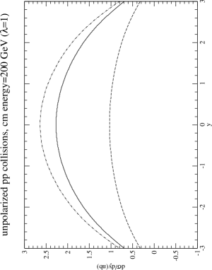
Figure 2: Differential rapidity distributions for $J/\psi$ production at $\sqrt{s}$ = 200 GeV. The solid, dashed and dot-dashed lines, each to be multiplied by a scale factor of 200, are for unpolarized p-p collisions with $J/\psi$ helicities $\lambda$ = 1 in scenarios 1, 2 and 3 respectively.

Therefore we choose three scenarios.
1.  $<{\cal{O}}^{J/\psi}_{8}(^{1}S_{0})>$ and $<{\cal{O}}^{J/\psi}_{8}(^{3}P_{0})>/m^{2}$ are roughly equal, so we set both to 0.0087 GeV³.
2.  $<{\cal{O}}^{J/\psi}_{8}(^{1}S_{0})>$ is much larger than $<{\cal{O}}^{J/\psi}_{8}(^{3}P_{0})>/m^{2}$ so we set the former to 0.039 GeV³ and the latter to zero.
3.  $<{\cal{O}}^{J/\psi}_{8}(^{1}S_{0})>$ is much smaller than $<{\cal{O}}^{J/\psi}_{8}(^{3}P_{0})>/m^{2}$ so we set the former to zero and the latter to 0.01125 GeV³.
In all three cases $M^{J/\psi}(^{1}S_{0}^{(8)},{}^{3}P_{0}^{(8)})\approx 0.039\,{\rm GeV}^{3}$, which is the central value in BK for GRV leading order (LO) parton densities grv95 . We also take $<{\cal{O}}^{J/\psi}_{8}(^{3}S_{1})>=0.0112\,{\rm GeV}^{3}$ in agreement with the value in BK . Note that these values can still vary up and down by approximately fifty percent.

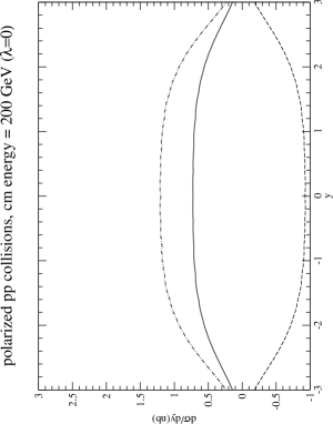
Figure 3: Differential rapidity distributions for $J/\psi$ production at $\sqrt{s}$ = 200 GeV. The solid, dashed and dot-dashed lines are for polarized p-p collisions with $J/\psi$ helicities $\lambda$ = 0 in scenarios 1, 2 and 3 respectively.

The central arm (forward arm) electron (muon) detector at the PHENIX experiment covers the $J/\psi$ rapidity range $-0.5<~{}y~{}<0.5$ ($1<~{}|y|~{}<2$). We will present our differential rapidity distributions and spin asymmetries for $J/\psi$ and $\psi^{\prime}$ production with helicities $\lambda$ = 1 and 0 in unpolarized and polarized p-p collisions at $\sqrt{s}$ = 200 GeV and 500 GeV in the above detector acceptance ranges.

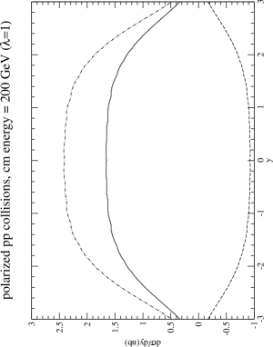
Figure 4: Differential rapidity distributions for $J/\psi$ production at $\sqrt{s}$ = 200 GeV. The solid, dashed and dot-dashed lines are for polarized p-p collisions with $J/\psi$ helicities $\lambda$ = 1 in scenarios 1, 2 and 3 respectively.

We take the charm quark mass $m$=1.5 GeV and the mass factorization scale equal to $2m$. Several groups have produced polarized parton density sets GS ,grsv and blbo . We choose the GRV unpolarized LO parton densities grv98 and the GRSV grsv polarized densities. The latter authors have a standard scenario and a valence scenario. For simplicity we choose the former. Therefore we always use the LO four flavour sets (for the u, d, s and g partons) and we set $n_{f}=4$ in the one-loop running coupling constant and the parton densities. For both parton density sets we use $\Lambda^{\rm LO}_{4}=175$ MeV, so that $\alpha_{s}^{\rm LO}(m_{Z})=0.121$ at the mass of the Z.

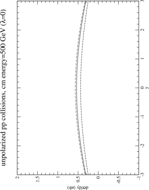
Figure 5: Differential rapidity distributions for $J/\psi$ production at $\sqrt{s}$ = 500 GeV. The solid, dashed and dot-dashed lines, each to be multiplied by a scale factor of 1000, are for unpolarized p-p collisions with $J/\psi$ helicities $\lambda$ = 0 in scenarios 1, 2 and 3 respectively.

We first choose helicity $\lambda=0$ which eliminates contributions from $<{\cal{O}}^{J/\psi}_{8}(^{3}S_{1})>$ in eqns. (26) and (27). Note that this contribution only appears in the quark-antiquark channel. In Fig. 1 we present the rapidity differential distributions for $J/\psi$ production with $\lambda=0$ in unpolarized p-p collisions at $\sqrt{s}$ = 200 GeV. The solid, dashed and dot-dashed lines, each to be multiplied by 200, are the differential distributions for the scenarios 1, 2 and 3 respectively. As expected there is very little difference between them. Note that the $y$ axis is taken from -1 to +3 as in the case of the polarized plots, which will be shown shortly. Fig. 2 contains the corresponding distributions when $\lambda=1$. Now $<{\cal{O}}^{J/\psi}_{8}(^{3}S_{1})>$ contributes to eqn. (27) and is responsible for the tiny difference between the results for the second scenarios (the dashed lines). From this we conclude that the gluon-gluon contributions completely dominate the quark-antiquark contribution for this cm energy. The larger differences between the other results are due to the changes in the prefactors multiplying the octet contributions in eqn. (27).

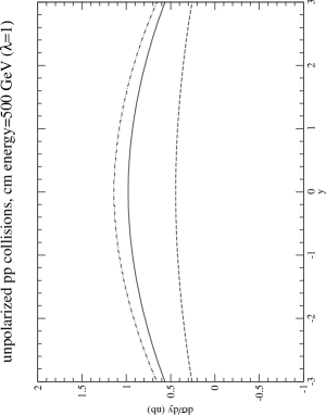
Figure 6: Differential rapidity distributions for $J/\psi$ production at $\sqrt{s}$ = 500 GeV. The solid, dashed and dot-dashed lines, each to be multiplied by a scale factor of 1000, are for unpolarized p-p collisions with $J/\psi$ helicities $\lambda$ = 1 in scenarios 1, 2 and 3 respectively.

We now give the corresponding results for longitudinally polarized p-p collisions at the same cm energy using eqn. (26). Fig. 3 has $\lambda=0$ and Fig. 4 has $\lambda=1$. In both cases scenario 2, where $<{\cal{O}}^{J/\psi}_{8}(^{3}P_{0})>/m^{2}=\,0$, yields, as expected from the signs in eqn. (26), negative results. We conclude that the polarized results are at least a factor of 200 lower then the unpolarized ones but they could be much smaller due to cancellations between the color octet contributions in eqn. (26) and could possibly be negative.

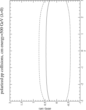
Figure 7: Differential rapidity distributions for $J/\psi$ production at $\sqrt{s}$ = 500 GeV. The solid, dashed and dot-dashed lines are for polarized p-p collisions with $J/\psi$ helicities $\lambda$ = 0 in scenarios 1, 2 and 3 respectively.

In Figs. 5 - 8 we repeat the plots in Figs. 1 - 4 but for $\sqrt{s}=500$ GeV. This time we divide the unpolarized values by 1000 so that they fit on the same scales as the polarized ones. Also we choose the $y$-axis from -1 to +2 so that the polarized and unpolarized plots can be easily compared. The comments we made earlier about Figs. 1 - 4 are also valid for these plots. Here we see that that the polarized values are at least a factor of 1000 times smaller than the unpolarized ones, which is due to the rapid rise of the unpolarized gluon density at small $x$, but again they could be even smaller due to cancellations between the color octet contributions.

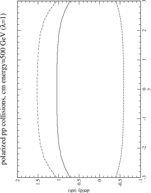
Figure 8: Differential rapidity distributions for $J/\psi$ production at $\sqrt{s}$ = 500 GeV. The solid, dashed and dot-dashed lines are for polarized p-p collisions with $J/\psi$ helicities $\lambda$ = 1 in scenarios 1, 2 and 3 respectively.

For completeness we give in Fig.9 the rapidity distributions for the spin asymmetry $A_{LL}$ defined in eq. (28) for $J/\psi$ production in p-p collisions at $\sqrt{s}$ = 200 GeV. This is for the scenario 1. The solid and dotted lines are for helicities $\lambda=1$ and 0 respectively. We see that the ratios are rather flat over the central rapidity range. For scenario 2 $A_{LL}$ is negative and roughly the same in absolute value. For scenario 3 $A_{LL}$ is positive and about the same. Therefore we do not show the latter two cases.

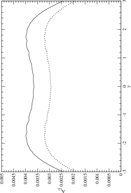
Figure 9: Differential rapidity distributions for $A_{LL}$ at $\sqrt{s}$ = 200 GeV in scenario 1. The solid and dotted lines are for helicities $\lambda=1$ and 0 respectively.

Finally Fig. 10 contains the rapidity distributions of the spin asymmetries $A_{LL}$ for $J/\psi$ production in p-p collisions at $\sqrt{s}$ = 500 GeV. The solid and dotted lines are the spin asymmetries for helicities $\lambda=1$ and 0 respectively. The ratio is also rather flat and smaller than in Fig. 9, which is due to the increase in the unpolarized gluon density at small $x$. We do not give the plots for scenarios 2 and 3 as they are similar in absolute magnitude.

Let us now consider $\psi^{\prime}$ production. Central values for $<{\cal{O}}^{\psi^{\prime}}_{8}(^{3}S_{1})>$ and the combination

$$M^{\psi^{\prime}}(^{1}S_{0}^{(8)},{}^{3}P_{0}^{(8)})=<{\cal{O}}^{\psi^{\prime}}_{8}(^{1}S_{0})>+3.5<{\cal{O}}^{\psi^{\prime}}_{8}(^{3}P_{0})>/m^{2}\,,$$ (30)

together with reasonable error ranges from both statistical and theoretical uncertainties are given in BK . However we note that only the former, equal to 0.0046 GeV³, is derived from data analysis while the latter is not. The data were simply not good enough so it was assumed that the ratios of the above color combinations are the same for the $J/\psi$ and $\psi^{\prime}$ respectively. However we have seen that the contribution from $<{\cal{O}}^{\psi^{\prime}}_{8}(^{3}S_{1})>$ in the quark-antiquark channel is completely negligible compared to the other color octet contributions from the gluon-gluon channel in this energy range. Hence we only need to look at the ratios in BK to determine the reduction factor for the rapidity distributions for $\psi^{\prime}$ production. This is 3.5 so all plots given above in Figs. 1 - 8 can be used for $\psi^{\prime}$ production by simply dividing them by this number. The $A_{LL}$ ratio plots in Figs. 9 and 10 are not affected since this factor cancels between the numerator and denominator.

In this paper we have calculated inclusive production cross sections and spin asymmetries for heavy quarkonium states with definite helicities in polarized proton-proton collisions using the non-relativistic QCD color-octet mechanism. We have presented the LO results for $J/\psi$ and $\psi^{\prime}$ rapidity differential distributions with definite helicities in polarized p-p collisions at $\sqrt{s}$ = 200 GeV and 500 GeV at the RHIC within the PHENIX detector acceptance range. One can see from the figures that the contributions from the $\lambda=\pm 1$ states dominate. This is explained by the fact that the RHIC is a p-p collider so the contribution from the quark-antiquark channel is small compared to the contribution from the gluon-gluon channel and the coefficient in front of the $<{\cal{O}}^{\psi^{\prime}}_{8}(^{3}P_{0})>$ term in eqn. (26) is larger for $\lambda=1$ than for $\lambda=0$. The PHENIX experiment should be able to measure these spin asymmetries. The study of heavy quarkonium production with definite helicities in polarized p-p collisions is unique because it tests the spin transfer processes in perturbative QCD. As Tevatron data for heavy quarkonium polarization expt is not explained by the color octet mechanism CDFpolarization , it will be interesting to compare these theoretical results with the future experimental data at RHIC to test the NRQCD color octet heavy quarkonium production mechanism with respect to polarization. A calculation of the $p_{T}$ distribution in heavy quarkonium production with definite polarization states in polarized p-p collisions at RHIC should also show interesting features.

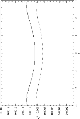
Figure 10: Differential rapidity distributions for $A_{LL}$ at $\sqrt{s}$ = 500 GeV in scenario 1. The solid and dotted lines are for helicities $\lambda=1$ and 0 respectively.