CERN-PH-TH/2005-173, UMN–TH–2416/05, FTPI–MINN–05/43, ACT-09-05, MIFP-05-23

On the Higgs Mass in the CMSSM

John Ellis¹, Dimitri Nanopoulos², Keith A. Olive³ and Yudi Santoso^{4 1}TH Division, PH Department, CERN, Geneva, Switzerland
²George P. and Cynthia W. Mitchell Institute for Fundamental Physics,
Texas A&M University, College Station, TX 77843, USA;
Astroparticle Physics Group, Houston Advanced Research Center (HARC), Mitchell Campus, Woodlands, TX 77381, USA;
Academy of Athens, Division of Natural Sciences, 28 Panepistimiou Avenue, Athens 10679, Greece
³William I. Fine Theoretical Physics Institute,
University of Minnesota, Minneapolis, MN 55455, USA
⁴Department of Physics and Astronomy, University of Victoria,
Victoria, BC, V8P 1A1, Canada;
Perimeter Institute of Theoretical Physics, Waterloo, ON, N2J 2W9, Canada

Abstract

We estimate the mass of the lightest neutral Higgs boson $h$ in the minimal supersymmetric extension of the Standard Model with universal soft supersymmetry-breaking masses (CMSSM), subject to the available accelerator and astrophysical constraints. For $m_{t}=174.3$ GeV, we find that $114~{}{\rm GeV}<m_{h}<127$ GeV and a peak in the $\tan\beta$ distribution $\simeq 55$. We observe two distinct peaks in the distribution of $m_{h}$ values, corresponding to two different regions of the CMSSM parameter space. Values of $m_{h}<119$ GeV correspond to small values of the gaugino mass $m_{1/2}$ and the soft trilinear supersymmetry-breaking parameter $A_{0}$, lying along coannihilation strips, and most of the allowed parameter sets are consistent with a supersymmetric interpretation of the possibly discrepancy in $g_{\mu}-2$. On the other hand, values of $m_{h}>119$ GeV may correspond to much larger values of $m_{1/2}$ and $A_{0}$, lying in rapid-annihilation funnels. The favoured ranges of $m_{h}$ vary with $m_{t}$, the two peaks being more clearly separated for $m_{t}=178$ GeV and merging for $m_{t}=172.7$ GeV. If the $g_{\mu}-2$ constraint is imposed, the mode of the $m_{h}$ distribution is quite stable, being $\sim 117$ GeV for all the studied values of $m_{t}$.

CERN-PH-TH/2005-173

September 2005

1 Introduction

One of the characteristic predictions of the minimal supersymmetric extension of the Standard Model (MSSM) is the mass of the lightest neutral Higgs boson $h$, which is expected to be $m_{h}\mathrel{\raise 1.29167pt\hbox{$<$\kern-7.5pt\lower 4.30554pt\hbox{$\sim$}}}150$ GeV [1]. This is very consistent with the range $m_{h}\mathrel{\raise 1.29167pt\hbox{$<$\kern-7.5pt\lower 4.30554pt\hbox{$\sim$}}}200$ GeV that is favoured by global analyses of the available precision electroweak data [2]. Various studies have shown that the lightest neutral MSSM Higgs boson is very likely to be discovered at the LHC, and possibly at the Fermilab Tevatron collider. It is therefore interesting to attempt to refine the MSSM prediction for $m_{h}$, and to consider what one would learn from a measurement of the $h$ mass [3].

We study these questions within the constrained version of the MSSM (CMSSM), in which the soft supersymmetry-breaking scalar masses $m_{0}$ and gaugino masses $m_{1/2}$ are each assumed to be universal at some GUT input scale, as are the trilinear soft supersymmetry-breaking parameters $A_{0}$. We impose on the CMSSM the available phenomenological constraints from accelerator experiments, astrophysics and cosmology [4, 5], treating the supersymmetric interpretation of the anomalous magnetic moment of the muon, $g_{\mu}-2$, as an optional constraint, and interpreting the WMAP range for the cold dark matter density [6] as an upper bound: $\Omega_{\chi}h^{2}<0.129$.

We base our study on a statistical sampling of the CMSSM parameter space that is uniform in the $(m_{1/2},m_{0})$ plane for 100 GeV $<m_{1/2}<2$ TeV, $m_{0}<2$ TeV, $|A_{0}/m_{1/2}|<3$, $2<\tan\beta<58$ and $\mu>0$, assuming initially that $m_{t}=174.3$ GeV [7] and discussing later other possible values of $m_{t}$. We began with a random sample of over 320,000 CMSSM points: requiring the lightest supersymmetric particle (LSP) to be a neutralino brought the number down to somewhat over 260,000. As seen in Fig. 1(a), before imposing the various phenomenological constraints we find that $m_{h}$  is distributed between very low values $<110$ GeV and an upper limit $\sim 128$ GeV, with a single peak at $\sim 120$ GeV. The drop-off in the count at low $m_{h}$ is mainly related to our choice of a uniform measure in the CMSSM input parameters: because of the logarithmic dependence of $m_{h}$ on $m_{1/2}$ and $m_{0}$, low values of $m_{h}$ only occur at low values of $m_{1/2},m_{0}$ and $\tan\beta$. (We recall that $m_{h}$ evolves quickly as $m_{1/2}$ is increased at low $m_{1/2}$ and more slowly at large $m_{1/2}$.) The fall-off at large $m_{h}$ is largely due to our choice of 2 TeV as the upper limit on $m_{1/2}$. Extending this upper limit would slowly push the peak in Fig. 1(a) to the right, and the count at the peak would grow rapidly. Once again, because of the logarithmic dependence of $m_{h}$ on $m_{1/2}$, even a modest change in the position of the peak would require increasing the upper limit on $m_{1/2}$ substantially.

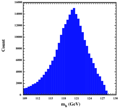
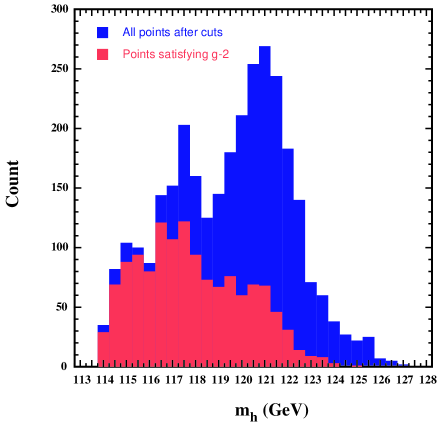
Figure 1: The distribution of the mass of the lightest neutral Higgs boson, $m_{h}$, in the CMSSM (a) before applying the accelerator cuts and the WMAP relic density constraint, and (b) after applying these constraints. In the latter case, the red (light) histogram shows the points favoured by the optional $g_{\mu}-2$ constraint. We assume $m_{t}=174.3$ GeV in both panels.

We next apply a series of constraints, including the LEP lower limit on the chargino mass of 104 GeV, $b\to s\gamma$ [9] and the limit on $\Omega_{\chi}h^{2}$ that was discussed above, as well as the the direct experimental limit on $m_{h}$ of $\sim 114$ GeV [10] . The most severe cut on the sample, by far, is that due to the relic density, which for most points exceeds the WMAP upper limit. When all cuts are applied our sample is reduced to 3075 points, which are plotted in Fig. 1(b). Most of the range in $m_{h}$ is still available after imposing the various phenomenological constraints, as seen in Fig. 1(b). However, we see that the distribution of $m_{h}$ within this range exhibits significant structures, with peaks at $m_{h}\simeq 121$ and $117$ GeV, and a dip at $m_{h}\simeq 119$ GeV.

In the rest of this paper, we explain the origins of these features, describe the domains of the CMSSM parameter space that populate these peaks in the $m_{h}$ distribution, and discuss the effects of imposing the optional $g_{\mu}-2$ constraint [12] and varying $m_{t}$. The peaked structures in $\tan\beta$ and $m_{h}$ reflect different processes that might reduce the density of supersymmetric relics $\chi$ into the range allowed by WMAP and other observations : either coannihilations with sleptons, most importantly the lighter stau: ${\tilde{\tau}}_{1}$ [14], or rapid annihilations: $\chi\chi$ via the heavier neutral Higgs bosons $A,H$ [15], or (exceptionally) rapid annihilations: $\chi\chi$ via the lightest neutral Higgs bosons $h$ [16].

The structures in the $m_{h}$ distribution imply that, once $m_{t}$ is better known from Tevatron and/or LHC measurements and assuming the CMSSM framework , a measurement of $m_{h}$ at the LHC or Tevatron might enable one to estimate ranges for the values of $m_{1/2},A_{0}$ and $\tan\beta$, even if sparticles themselves are not yet discovered. If sparticles are discovered, confronting their masses with the ranges inferred from $m_{h}$ will be a crucial test of the CMSSM framework.

2 Effects of Phenomenological Constraints on the CMSSM Parameter Space

As already mentioned, we have sampled uniformly the $(m_{1/2},m_{0})$ plane for $m_{1/2},m_{0}<2$ TeV, $|A_{0}/m_{1/2}|<3$, $2<\tan\beta<58$ and $\mu>0$ , assuming $m_{t}=174.3$ GeV as our default . As $\tan\beta$ is increased, there is an increasing fraction of sample points that do not yield consistent electroweak vacua. Nevertheless, the consistent solutions are distributed quite smoothly in $\tan\beta$ before applying the accelerator and cosmological cuts, as seen in panel (a) of Fig. 2. However, after applying the cuts, the distribution in $\tan\beta$ is far from uniform, as seen in panel (b) of Fig. 2. The distribution of allowed models is sharply peaked towards large $\tan\beta$, with a relatively small tail surviving below $\tan\beta\sim 20$. This observation holds for both the general sample and the $(g_{\mu}-2)$-friendly subsample , shown as the light (red) shaded histogram in panel (b).

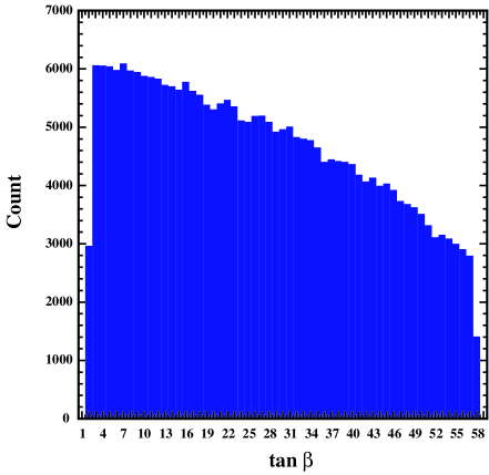
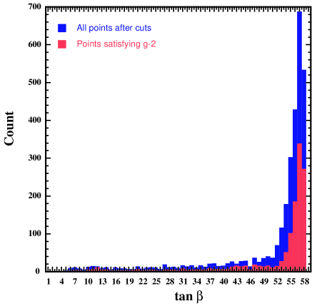
Figure 2: (a) The distribution in $\tan\beta$ of the sample points shown in Fig. 1(a), before the accelerator and WMAP constraints are applied, and (b) their distribution after applying these phenomenological constraints. In the latter, we see that the distribution of $g_{\mu}-2$-friendly points (coloured red/grey) is similar to that of the total sample.

The preference for large $\tan\beta$ is an understandable consequence of the interplay of the various accelerator and cosmological constraints. For example, the cosmological upper limit on the supersymmetric relic density in the coannihilation region imposes an upper limit on $m_{1/2}$ that is significantly relaxed at large $\tan\beta$, in particular by rapid $\chi\chi\to A,H$ annihilation. Moreover, the funnels due to the rapid-annihilation processes $\chi\chi\to H,A$ are broader than the coannihilation strips that define the acceptable cosmological regions at lower $\tan\beta$. We also note that the range of small values of $m_{1/2}$ that is excluded by the experimental lower limit on $m_{h}$ diminishes as $\tan\beta$ increases, and recall that the predominance of high $\tan\beta$ in satisfying constraints was clearly seen in a likelihood analysis [17] when comparing regions of high likelihood for $\tan\beta=10$ and 50.

Panel (a) of Fig. 3 displays the allowed points in the $(A_{0},\tan\beta)$ plane. We see that they gather into three clusters: one centered around $A_{0}=0$ that extends to small values of $\tan\beta$, and two at large values of $|A_{0}|$ that are concentrated at larger $\tan\beta$, particularly for $A_{0}<0$. As seen in panel (b) of Fig. 3, these accumulations populate different regions of $m_{h}$. Specifically, the points with $m_{h}\in(114,119)$ GeV, which populate the low-mass peak in Fig. 1(b), have relatively low values of $A_{0}$, most of which are negative. On the other hand, points with $A_{0}<-2$ TeV generally have $m_{h}\in(119,122)$ GeV and points with $A_{0}>1$ TeV have $m_{h}\in(122,127)$ GeV. Between these wings, there are addditionally some low-$|A_{0}|$ points with $m_{h}\in(119,124)$ GeV. Thus, the higher-mass peak in Fig. 1(b) receives contributions from all regions of $A_{0}$. We also see in Fig. 1(b) that essentially all the low-mass points are $(g_{\mu}-2)$-friendly (shaded red/grey), that only some of the high-mass points with $A_{0}>-2$ TeV are $(g_{\mu}-2)$-friendly, and that none of the points with $A_{0}<-2$ TeV are $(g_{\mu}-2)$-friendly.

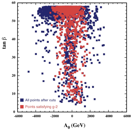
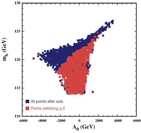
Figure 3: (a) The distribution in the $(A_{0},\tan\beta)$ plane of the sample points shown in Fig. 1(b) that survive the accelerator and WMAP constraints, and (b) a scatter plot of these points in the $(A_{0},m_{h})$ plane. The $(g_{\mu}-2)$-friendly points are coloured red (grey).

3 Interpretation of Features in the $m_{h}$ Distribution

The origins of many of these features can be understood qualitatively by referring to the various $(m_{1/2},m_{0})$ planes displayed in Fig. 2 of [18] for different values of $\tan\beta$ and $A_{0}$. Updated planes for the case $\tan\beta=55$, whose importance can be seen from panel (b) of Fig. 2 and panel (a) of Fig. 3, are shown in Fig. 4. When $\tan\beta\mathrel{\raise 1.29167pt\hbox{$<$\kern-7.5pt\lower 4.30554pt\hbox{$\sim$}}}45$ and $\mu>0$ as assumed here, the regions allowed by WMAP and the other constraints are essentially narrow coannihilation strips that decrease in width as $m_{1/2}$ increases, terminating when $m_{1/2}\sim 1000$ GeV. In most of these regions, $|A_{0}|\mathrel{\raise 1.29167pt\hbox{$<$\kern-7.5pt\lower 4.30554pt\hbox{$\sim$}}}1000$ GeV also, so these points populate the central $A_{0}\sim 0$ region in Fig. 3(b). Therefore, they provide the majority of the models in the low-mass peak in Fig. 1(b), but also a tail extending under the higher-mass peak, as seen in panel (b) of Fig. 3. These coannihilation strips are also the dominant features for $\tan\beta=55$ when $A_{0}>0$, as seen in panel (a) of Fig. 4 by the two examples for $A_{0}=+m_{1/2},+2m_{1/2}$.

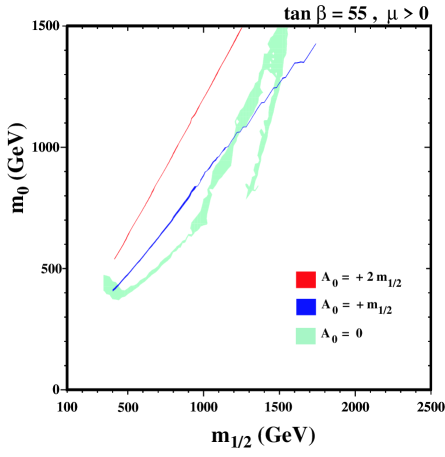
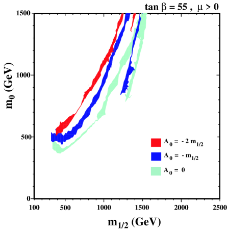
Figure 4: Regions in the $(m_{1/2},m_{0})$ planes for $\tan\beta=55$, as calculated for $m_{t}=174.3$ GeV using the latest version of the SSARD code [19]. Note the narrow coannihilation strips for $A_{0}>0$ in panel (a) and the broader rapid-annihilation funnels for $A_{0}<0$ shown in panel (b).

However, a second class of features is visible in Fig. 2 of [18] when $\tan\beta\mathrel{\raise 1.29167pt\hbox{$>$\kern-7.5pt\lower 4.30554pt\hbox{$\sim$}}}50$, namely rapid-annihilation funnels at large $m_{1/2}$, as updated in panels (a, b) of Fig. 4 for $A_{0}=0,-m_{1/2},-2m_{1/2}$. These funnel regions populate the high-mass peak in Fig. 1(b). The funnels are typically broader than the coannihilation strips, and therefore have a larger weighting in the constant-density sampling of the $(m_{1/2},m_{0})$ plane that we have made in this paper. As a result, the larger values of $\tan\beta$ have a strong weight in the sample of models surviving the accelerator and WMAP constraints that we showed in Fig. 2. We recall that we retain in our analysis points whose relic density $\Omega_{\chi}h^{2}$ falls below the range favoured by WMAP [6], which typically have slightly lower values of $m_{0}$ than along the coannihilation strips, while remaining within the region where the LSP is the lightest neutralino $\chi$, and lie inside the rapid-annihilation funnels. Restricting our plots to points with $\Omega_{\chi}$ within the WMAP range would reduce the statistics in our plots, but not alter their basic features. The weight of the rapid-annihilation points could be diminished if one used a different sampling procedure, e.g., if one gave less weight to regions of parameter space with large $m_{1/2}$ and/or $m_{0}$, and hence $|A_{0}|$, as might be motivated by fine-tuning considerations. However, the ‘twin-peak’ structure of the $m_{h}$ distribution would survive any smooth reweighting of parameter space.

The rapid-annihilation funnels are responsible for the dense cluster of models at large $\tan\beta$ and $A_{0}<-2$ TeV in panel (a) of Fig. 3, which have $m_{h}>119$ GeV as seen in panel (b) of Fig. 3, and hence populate the higher peak in the Higgs mass distribution in Fig. 1. It is also clear from Figs. 1 and 3 that the basic feature of a doubly-peaked Higgs mass distribution linked to different ranges of $A_{0}$ would also survive any smooth reweighting of the parameter space.

As discussed in [18] and seen in Fig. 4, the locations of the rapid-annihilation funnels are very sensitive to $A_{0}$, reflecting the sensitivity of $m_{A,H}$ to this parameter (among others). Starting from the $A_{0}=0$ case where the funnel extends above $m_{1/2}\sim 1000$ GeV for $m_{t}=174.3$ GeV, the funnel moves to smaller $m_{1/2}$ as $A_{0}$ decreases and merges progressively with the coannihilation strip. On the other hand, no funnels are visible for $A_{0}$ sufficiently $>0$. The WMAP regions for $A_{0}=\pm 2m_{1/2}$ provide points in Fig. 3 with extreme positive and negative values of $A_{0}$, respectively. The different breadths of these regions explain the asymmetry in panel (b) of Fig. 3, in particular. Indeed, for $A_{0}>0$ these points are simply continuations of the coannihilation strips. As seen in Fig. 3, some of these points are $(g_{\mu}-2)$-friendly, and provide the tail under the high-mass peak in Fig. 1.

We now consider the $(m_{1/2},A_{0})$ planes shown in Fig. 5, where panel (a) shows the combination of all vales of $\tan\beta$, and panel (b) shows only models with $\tan\beta>50$. These panels update analogous plots in [18], and display significant differences due to the reduction in $m_{t}$ from 178 GeV to 174.3 GeV and improvements in the treatment of vacuum stability requirements. Previously, we had seen a clear separation between ‘fins’ at $A_{0}\sim\pm 1.5m_{1/2}$ and a ‘torso’ at $A_{0}\sim 0$, which has vanished apart (possibly) from a vestigial fin at $A_{0}>2$ TeV that is more visible at large $\tan\beta$. We also note the ap pearance of a small ‘head’ with a ‘tooth’ at $m_{1/2}\mathrel{\raise 1.29167pt\hbox{$<$\kern-7.5pt\lower 4.30554pt\hbox{$\sim$}}}150$ GeV and $A_{0}\sim 0$, which is due to points with $m_{\chi}\sim m_{h}/2$, whose relic density falls within the WMAP range thanks to rapid annihilation through the light CMSSM Higgs pole [16]. These points have $m_{\chi^{\pm}}$ very close to the LEP lower limit, and might be accessible to the Tevatron.

We see in panel (a) of Fig. 5 that the points with $m_{h}<119$ GeV (darker blue/black and red/grey colours) cluster at $m_{1/2},A_{0}<1$ TeV and $A_{0}>-3$ TeV. Almost all these points make a supersymmetric contribution to $g_{\mu}-2$ that could explain the possible discrepancy between experiment and the Standard Model calculation based on $e^{+}e^{-}$ data (indicated in red/grey). On the other hand, only a small fraction of the models with $m_{h}>119$ GeV (pale colours) are compatible with this supersymmetric interpretation of $g_{\mu}-2$ (pink/light grey). As seen in panel (b) of Fig. 5, all the parameter sets with $\tan\beta>50$ have $m_{h}>119$ GeV. The $(g_{\mu}-2)$-friendly points are concentrated at $m_{1/2}\mathrel{\hbox to0.0pt{\raise 2.15277pt\hbox{$<$}\hss}{\lower 2.15277pt\hbox{$\sim$}}}1$ TeV.

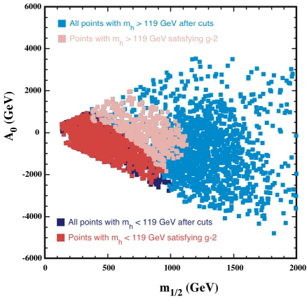
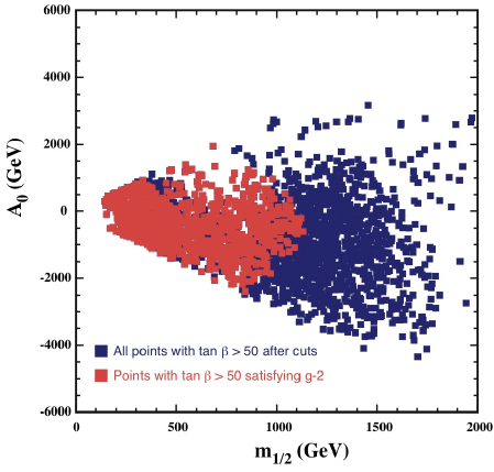
Figure 5: (a) The distribution in the $(m_{1/2},A_{0})$ plane of the points shown in Fig. 1(b) that satisfy the accelerator and WMAP constraints, separated into the low-$m_{h}$ region (blue points) and the high-$m_{h}$ region (red points). (b) The distribution in the $(m_{1/2},A_{0})$ plane of points with $\tan\beta>50$.

This analysis can be used as a diagnostic tool when the Higgs boson is discovered at the Tevatron or the LHC, at least within the CMSSM framework and assuming that $m_{t}=174.3$ GeV. This framework would be invalidated if $m_{h}>127$ GeV. On the other hand, if the Higgs boson is discovered with a mass $m_{h}<119$ GeV, one can infer from Fig. 5(a) that both $m_{1/2}$ and $A_{0}$ must be small, and that supersymmetry is likely to lie along a coannihilation strip. On the other hand, if $m_{h}>119$ GeV, supersymmetry may well have chosen a rapid-annihilation funnel.

4 Potential Impact of $g_{\mu}-2$

We now comment further on the potential impact of imposing the $g_{\mu}-2$ constraint [12], which we treat as optional. We see in Fig. 1(b) that this constraint would suppress the high-$m_{h}$ peak, while retaining most of the low-$m_{h}$ models. The suppression of the high-$m_{h}$ peak is a consequence of the removal of points with large $m_{1/2}$ and/or $m_{0}$ that would make a very small contribution to $g_{\mu}-2$, many of which are in the rapid-annihilation funnels. A similar effect reduces also the upper part of the low-$m_{h}$ peak, but the coannihilation strips would be less affected by the $g_{\mu}-2$ constraint. On the other hand, as seen in Fig. 2, imposing the $g_{\mu}-2$ constraint would not alter the statistical preference for large $\tan\beta$. As we see in Fig. 3, imposing the $g_{\mu}-2$ constraint would disfavour models with large negative $A_{0}$, as well as many with large positive $A_{0}$, but some models with large $\tan\beta$ and a small $A_{0}$ would survive.

5 Dependence on $m_{t}$

In all the above, we have assumed that $m_{t}=174.3$ GeV [7]. The central value was formerly 178 GeV [20], and the current central value is $m_{t}=172.7\pm 2.9$ GeV [21], following significant evolution during recent months. In view of this and the remaining experimental uncertainty, we have also considered the dependence of the above analysis on $m_{t}$. We recall that $\Delta m_{h}\sim 1$ GeV for $\Delta m_{t}=1$ GeV in theoretical calculations, and that the parameter regions allowed by WMAP vary quite considerably with $m_{t}$, particularly in the rapid-annihilation funnel region, as seen in Fig. 1 of [18]. Specifically, this region moves to smaller (larger) $m_{1/2}$ for smaller (larger) $m_{t}$. As was already mentioned, the coannihilation strips mainly populate the low-mass peak in Fig. 1 whereas the high-mass peak is largely due to the rapid-annihilation funnels. Accordingly, we would expect these peaks to be more separated at large $m_{t}$ than at smaller values. Precisely this effect is seen in the two panels of Fig. 6. We see in panel (a) that the upper peak in Fig. 1(b) shifts upwards by $\sim 4$ GeV if $m_{t}=178$ GeV [20], and is very clearly separated from the low-mass peak. Correspondingly, the upper limit on $m_{h}$ increases to 130 GeV. On the other hand, we see in panel (b) of Fig. 6 that the two peaks merge for $m_{t}=172.7$ GeV [21], and the upper limit on $m_{h}$ decreases to 126 GeV. Likewise, many of the other features discussed previously in this paper become more (less) pronounced for larger (smaller) $m_{t}$.

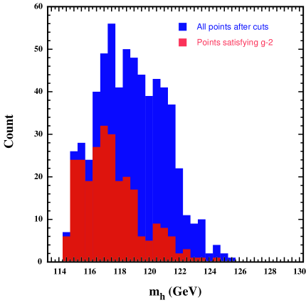
Figure 6: As for panel (b) of Fig. 1, but assuming (a) $m_{t}=178$ GeV and (b) $m_{t}=172.7$ GeV.

By the time the Higgs boson is discovered, we expect $m_{t}$ to be known with considerably greater precision than the present uncertainty $\delta m_{t}\simeq 2.9$ GeV. Once $m_{t}$ is known with an accuracy $\delta m_{t}\mathrel{\raise 1.29167pt\hbox{$<$\kern-7.5pt\lower 4.30554pt\hbox{$\sim$}}}2$ GeV, and assuming that the accuracy of theoretical calculations in the CMSSM can be brought to the same level, there will be no theoretical ambiguity between the Higgs mass peaks, and diagnosis of the supersymmetric parameters will indeed be possible along the lines discussed in the previous Section.

As in the case $m_{t}=174.3$ GeV shown in panel (a) of Fig. 1, for $m_{t}=178$ GeV the effect of imposing the $g_{\mu}-2$ constraint would also be to remove the high-mass peak, leaving a plateau extending from $m_{t}\sim 118$ GeV to $\sim 127$ GeV. The low-mass-peak would also be reduced, but most of the intermediate plateau for $m_{t}=178$ GeV would survive the $g_{\mu}-2$ constraint. In the case of $m_{t}=172.7$ GeV shown in panel (b), there is a more pronounced peak at $m_{t}\sim 117$ GeV and a tail extending to $\sim 124$ GeV. It is striking that, whatever the value of $m_{t}$, the mode of the $m_{h}$ distribution is relatively stable at $\sim 117$ GeV and that the upper limit on $m_{h}$ also remains relatively stable around 125 GeV, if the $g_{\mu}-2$ constraint is imposed.

6 Conclusions

We have shown that the available experimental and cosmological constraints on the CMSSM allow only a limited range of $m_{h}$. If $m_{t}=174.3$ GeV, this is $<127$ GeV without the $g_{\mu}-2$ constraint and $<124$ GeV if it is imposed. If $g_{\mu}-2$ is not imposed, we find twin peaks in the $m_{h}$ distribution at $m_{h}\sim 117,121$ GeV. The upper bound and the lower peak are quite insensitive to variations in $m_{t}$, whereas the upper peak is sensitive, and merges with the lower peak for low $m_{t}$. Large values of $\tan\beta\sim 55$ are favoured by our analysis, whether the $g_{\mu}-2$ constraint is applied, or not.

We have also shown in this paper that the mass of the lightest CMSSM Higgs boson may be a useful diagnostic tool for identifying the most likely regions of the CMSSM parameter space, even if sparticles are not (yet) discovered. This is because the CMSSM is divided into distinct coannihilation and rapid-annihilation regions, and measuring $m_{h}$ could provide us with a hint which alternative is chosen by Nature.

References

- [1] Y. Okada, M. Yamaguchi and T. Yanagida, Prog. Theor. Phys. 85 (1991) 1; Phys. Lett. B 262 (1991) 54; H. E. Haber and R. Hempfling, Phys. Rev. Lett. 66 (1991) 1815; J. R. Ellis, G. Ridolfi and F. Zwirner, Phys. Lett. B 257 (1991) 83; Phys. Lett. B 262 (1991) 477; A. Yamada, Phys. Lett. B 263, 233 (1991); M. Drees and M. M. Nojiri, Phys. Rev. D 45 (1992) 2482; P. H. Chankowski, S. Pokorski and J. Rosiek, Phys. Lett. B 274 (1992) 191; Phys. Lett. B 286 (1992) 307; A. Dabelstein, Z. Phys. C 67 (1995) 495 [arXiv:hep-ph/9409375]; M. Carena, J. R. Ellis, A. Pilaftsis and C. E. M. Wagner, Nucl. Phys. B 586 (2000) 92 [arXiv:hep-ph/0003180]; A. Katsikatsou, A. B. Lahanas, D. V. Nanopoulos and V. C. Spanos, Phys. Lett. B 501 (2001) 69 [arXiv:hep-ph/0011370].
-
[2]
G. Altarelli and M. W. Grunewald,
Phys. Rept. 403-404 (2004) 189
[arXiv:hep-ph/0404165].
updated in:
S. de Jong, talk given at EPS HEPP 2005, Lisbon, Portugal, July 2005, see:
http://lepewwg.web.cern.ch/LEPEWWG/misc/. - [3] J. R. Ellis, G. Ganis, D. V. Nanopoulos and K. A. Olive, Phys. Lett. B 502 (2001) 171 [arXiv:hep-ph/0009355].
- [4] J. Ellis, J.S. Hagelin, D.V. Nanopoulos, K.A. Olive and M. Srednicki, Nucl. Phys. B238 (1984) 453; see also H. Goldberg, Phys. Rev. Lett. 50 (1983) 1419.
- [5] J. R. Ellis, K. A. Olive, Y. Santoso and V. C. Spanos, Phys. Lett. B 565, 176 (2003) [arXiv:hep-ph/0303043]; H. Baer and C. Balazs, JCAP 0305, 006 (2003) [arXiv:hep-ph/0303114]; A. B. Lahanas and D. V. Nanopoulos, Phys. Lett. B 568, 55 (2003) [arXiv:hep-ph/0303130]; U. Chattopadhyay, A. Corsetti and P. Nath, Phys. Rev. D 68, 035005 (2003) [arXiv:hep-ph/0303201]; C. Munoz, arXiv:hep-ph/0309346; R. Arnowitt, B. Dutta and B. Hu, arXiv:hep-ph/0310103.
-
[6]
C. Bennett et al.,
Astrophys. J. Suppl. 148 (2003) 1,
astro-ph/0302207;
D. Spergel et al. [WMAP Collaboration], Astrophys. J. Suppl. 148 (2003) 175, astro-ph/0302209. - [7] CDF Collaboration, D0 Collaboration and Tevatron Electroweak Working Group, arXiv:hep-ex/0507006.
- [8] S. Heinemeyer, W. Hollik and G. Weiglein, Comp. Phys. Comm. 124 2000 76, hep-ph/9812320; Eur. Phys. J. C 9 (1999) 343, hep-ph/9812472. The codes are accessible via www.feynhiggs.de .
- [9] R. Barate et al. [ALEPH Collaboration], Phys. Lett. B 429 (1998) 169; S. Chen et al. [CLEO Collaboration], Phys. Rev. Lett. 87 (2001) 251807, hep-ex/0108032; P. Koppenburg et al. [Belle Collaboration], Phys. Rev. Lett. 93 (2004) 061803, hep-ex/0403004; K. Abe et al. [Belle Collaboration], Phys. Lett. B 511 (2001) 151, hep-ex/0103042; B. Aubert et al. [BABAR Collaboration], hep-ex/0207074; hep-ex/0207076; see also www.slac.stanford.edu/xorg/hfag/; C. Degrassi, P. Gambino and G. F. Giudice, JHEP 0012 (2000) 009 [arXiv:hep-ph/0009337]; M. Carena, D. Garcia, U. Nierste and C. E. Wagner, Phys. Lett. B 499 (2001) 141 [arXiv:hep-ph/0010003]; P. Gambino and M. Misiak, Nucl. Phys. B 611 (2001) 338; D. A. Demir and K. A. Olive, Phys. Rev. D 65 (2002) 034007 [arXiv:hep-ph/0107329]; T. Hurth, arXiv:hep-ph/0212304.
-
[10]
LEP Higgs Working Group for Higgs boson searches, OPAL Collaboration,
ALEPH Collaboration, DELPHI Collaboration and L3
Collaboration,
Phys. Lett. B 565 (2003) 61 [arXiv:hep-ex/0306033].
Search for neutral Higgs bosons at LEP, paper submitted to
ICHEP04, Beijing,
LHWG-NOTE-2004-01, ALEPH-2004-008, DELPHI-2004-042, L3-NOTE-2820,
OPAL-TN-744,
http://lephiggs.web.cern.ch/LEPHIGGS/papers/August2004_MSSM/index.html. - [11] J. R. Ellis, K. A. Olive and Y. Santoso, Phys. Lett. B 539 (2002) 107 [arXiv:hep-ph/0204192].
- [12] G. W. Bennett et al. [Muon g-2 Collaboration], Phys. Rev. Lett. 92 (2004) 161802 [arXiv:hep-ex/0401008]; M. Davier, S. Eidelman, A. Hocker and Z. Zhang, Eur. Phys. J. C 31 (2003) 503 [arXiv:hep-ph/0308213]; K. Hagiwara, A. D. Martin, D. Nomura and T. Teubner, arXiv:hep-ph/0312250; J. F. de Trocóniz and F. J. Ynduráin, arXiv:hep-ph/0402285; K. Melnikov and A. Vainshtein, arXiv:hep-ph/0312226; M. Passera, arXiv:hep-ph/0411168; A. Hocker, hep-ph/0410081.
- [13] C. Boehm, A. Djouadi and M. Drees, Phys. Rev. D 62 (2000) 035012 [arXiv:hep-ph/9911496]; J. R. Ellis, K. A. Olive and Y. Santoso, Astropart. Phys. 18 (2003) 395 [arXiv:hep-ph/0112113].
- [14] J. Ellis, T. Falk, and K.A. Olive, Phys. Lett. B444 (1998) 367 [arXiv:hep-ph/9810360]; J. Ellis, T. Falk, K.A. Olive, and M. Srednicki, Astr. Part. Phys. 13 (2000) 181 [Erratum-ibid. 15 (2001) 413] [arXiv:hep-ph/9905481]; R. Arnowitt, B. Dutta and Y. Santoso, Nucl. Phys. B 606 (2001) 59 [arXiv:hep-ph/0102181].
- [15] M. Drees and M. M. Nojiri, Phys. Rev. D 47 (1993) 376 [arXiv:hep-ph/9207234]; H. Baer and M. Brhlik, Phys. Rev. D 53 (1996) 597 [arXiv:hep-ph/9508321]; A. B. Lahanas, D. V. Nanopoulos and V. C. Spanos, Phys. Rev. D 62 (2000) 023515 [arXiv:hep-ph/9909497]; Mod. Phys. Lett. A 16 (2001) 1229 [arXiv:hep-ph/0009065]; H. Baer, M. Brhlik, M. A. Diaz, J. Ferrandis, P. Mercadante, P. Quintana and X. Tata, Phys. Rev. D 63 (2001) 015007 [arXiv:hep-ph/0005027]; J. R. Ellis, T. Falk, G. Ganis, K. A. Olive and M. Srednicki, Phys. Lett. B 510 (2001) 236 [arXiv:hep-ph/0102098].
- [16] A. Djouadi, M. Drees and J. L. Kneur, Phys. Lett. B 624 (2005) 60 [arXiv:hep-ph/0504090].
- [17] J. R. Ellis, K. A. Olive, Y. Santoso and V. C. Spanos, Phys. Rev. D 69 (2004) 095004 [arXiv:hep-ph/0310356].
- [18] J. R. Ellis, S. Heinemeyer, K. A. Olive and G. Weiglein, JHEP 0502 (2005) 013 [arXiv:hep-ph/0411216].
- [19] Information about this code is available from K. A. Olive: it contains important contributions from T. Falk, G. Ganis, J. McDonald, K. A. Olive, Y. Santoso and M. Srednicki.
-
[20]
V. Abazov et al. [D0 Collaboration],
Nature 429 (2004) 638,
hep-ex/0406031;
CDF Collaboration, D0 Collaboration and Tevatron Electroweak Working Group, hep-ex/0404010. - [21] CDF Collaboration, D0 Collaboration and Tevatron Electroweak Working Group, arXiv:hep-ex/0507091.