Paramagnetic Meissner Effect and Finite Spin Susceptibility
in an Asymmetric Superconductor

Abstract

A general analysis of Meissner effect and spin susceptibility of a uniform superconductor in an asymmetric two-component fermion system is presented in nonrelativistic field theory approach. We found that, the pairing mechanism dominates the magnetization property of superconductivity, and the asymmetry enhances the paramagnetism of the system. At the turning point from BCS to breached pairing superconductivity, the Meissner mass squared and spin susceptibility are divergent at zero temperature. In the breached pairing state induced by chemical potential difference and mass difference between the two kinds of fermions, the system goes from paramagnetism to diamagnetism, when the mass ratio of the two species increases.

I Introduction

It is well-known that there are two fundamental features of an electromagnetic superconductor, the zero resistance and the perfect diamagnetism. The latter is also called Meissner effectfetter . The key quantity describing the Meissner effect is the Meissner mass or penetration depth. In the language of gauge field theory, the Meissner mass is the mass of the electromagnetic field obtained through the spontaneous breaking of local $U(1)$ gauge symmetry, i.e., the Anderson-Higgs mechanismweinberg . Recently, the study on superconductivity is extended to color $SU(3)$ gauge field of Quantum Chromodynamics (QCD) at finite temperature and baryon densitycscreview .

In the linear response theory, the Meissner effect is defined in the static and long wave limit $\omega\rightarrow 0,\vec{\bf q}\rightarrow 0$ of the external magnetic potential $\vec{\bf A}(\vec{\bf q})$. From the microscopic BCS theory the electric current density can be expressed as fetter

$$\vec{\bf j}(\vec{\bf q})=-\vec{\bf A}(\vec{\bf q})\frac{ne^{2}}{mc}\left(1+\frac{\hbar^{2}}{3\pi^{2}mn}\int_{0}^{\infty}dpp^{4}\frac{\partial f(\epsilon_{\Delta})}{\partial\epsilon_{\Delta}}\right)\ ,$$ (1)

where $m,e,p$ and $n$ are respectively the mass, electric charge, momentum and density of electrons, $\epsilon_{\Delta}=\sqrt{(p^{2}/2m-\mu)^{2}+\Delta^{2}}$ is the quasi-particle energy with electric chemical potential $\mu$ and energy gap $\Delta$, and $f(x)$ the fermion distribution function. Since ${\partial f(\epsilon_{\Delta})}/{\partial\epsilon_{\Delta}}\leq 0$, the second term in the bracket on the right hand side is a paramagnetic one and cancels partially the diamagnetism characterized by the first term. However, the total Meissner mass squared keeps positive in normal superconductor with BCS pairing mechanism. At zero temperature, due to the limit ${\partial f(\epsilon_{\Delta})}/{\partial\epsilon_{\Delta}}\rightarrow-\delta(\epsilon_{\Delta})$, the second term in (1) disappears automatically, and there is no paramagnetic part. In addition to the perfect diamagnetism, the Meissner effect includes also the property of magnetic flux expulsion upon cooling through the critical temperature corresponding to the thermodynamic critical field.

Another quantity to describe the magnetization property of a superconductor is the spin susceptibility. Since an electron carries a Bohr magneton, a cold free electron gas exhibits Pauli paramagnetismfetter . However, at zero temperature the spin susceptibility $\chi$ of a metallic superconductor is zero, it does not possess Pauli paramagnetism. The physical picture is clear: The two electrons in a Cooper pair carry opposite spin. From the microscopic BCS theory, the spin susceptibility of a superconductor can be written asfetter

$$\frac{\chi}{\chi_{P}}=\frac{2}{3\pi^{2}}\frac{\epsilon_{F}}{n}\int_{0}^{\infty}dpp^{2}\left(-\frac{\partial f(\epsilon_{\Delta})}{\partial\epsilon_{\Delta}}\right)\ ,$$ (2)

where $\chi_{P}$ is the Pauli susceptibility of a normal electron gas, and $\epsilon_{F}$ the electron energy at the Fermi surface. Due to the above mentioned limit of ${\partial f(\epsilon_{\Delta})}/{\partial\epsilon_{\Delta}}$, the spin susceptibility of BCS type superconductor is zero at $T=0$. At finite temperature, $\chi$ is nonzero because of the thermo excitation in the superconductor.

The above discussed diamagnetic Meissner mass and zero spin susceptibility are only for normal BCS superconductor where the two fermions participating in a Cooper pair are symmetric, i.e., they have the same chemical potential, the same mass, and in turn the same Fermi surface. In many physical cases, however, the difference in chemical potentials, or number densities, or masses of the two kinds of fermions results in mismatched Fermi surfaces. Such physical systems can be realized in, for instance, a superconductor in an external magnetic fieldsarma or a strong spin-exchange fieldfulde ; larkin ; takada , an electronic gas with two species of electrons from different bandsliu , a superconductor with overlapping bandssuhl ; kondo , a system of trapped ions with dipolar interactionscirac , a mixture of two species of fermionic cold atoms with different densities and/or massesliu ; caldas , an isospin asymmetric nuclear matter with proton-neutron pairingsedrakian , and a neutral quark matter in dense QCDschafer ; alford ; rajagopal ; steiner ; alford2 ; huang ; abuki ; ruster ; blaschke ; shovkovy ; huang2 ; alford3 . In the study on superconductivity in an external magnetic field, Sarma sarma found an interesting spatial uniform state where there exist gapless modes. However, compared with the fully gapped BCS state, the Sarma state is energetically unfavored and therefore instable. A spatial non-uniform ground state where the order parameter has crystalline structure was also proposed for such type of superconductors by Fulde and Ferrell and Larkin and Ovchinnikov, the so-called LOFF state. In this ground state, the translational and the rotational symmetries of the system are spontaneously broken. Recently, the above spatial uniform ground state prompted new interest due to the work of Liu and Wilczekliu . They considered a system of two species of fermions with a large mass difference. The stability of the state has been discussed in many paperswu ; liu2 ; forbes ; shovkovy ; huang2 . It is now accepted that the Sarma instability can be avoided by two possible ways, finite difference in number densities of the two speciesforbes ; huang2 or a proper momentum structure of the attractive interaction between fermionsforbes . In these states, the dispersion relation of one branch of the quasi-particles has two zero points at momenta $p_{1}$ and $p_{2}$, and at these two points it needs no energy for quasi-particle excitations. The superfluid Fermi liquid phase in the regions $p<p_{1}$ and $p>p_{2}$ is breached by a normal Fermi liquid phase in the region $p_{1}<p<p_{2}$. The temperature behavior of such a breached pairing (BP) state is very different from that of a BCS state, the temperature corresponding to the maximum gap is not zero but finitesedrakian ; liao ; huang2 .

Since the dispersion relation controls the Meissner mass and the spin susceptibility, as shown above, it is natural to guess that the change in $\epsilon_{\Delta}$ in breached pairing superconductor will modify the Meissner effect and spin susceptibility significantly. Recently, it is found that the Meissner mass squared of some gluons in two flavor neutral color superconductor are negativehuang3 ; huang4 , which indicates that the quark matter in breached pairing state exhibits a paramagnetic Meissner effect (PME). In condensed matter physics, PME was observed first in high temperature superconductors such as ceramic samples of $Bi_{2}Sr_{2}CaCu_{2}O_{8+\delta}$svedlindh ; braunisch , and later in conventional superconductors such as Nbthompson ; kosti ; araujo ; barbara . It was suggested that the paramagnetic response might be a manifestation of $d$-wave superconductivityrice . However, it seems that it is not necessarily to do anything with the $d$-wave analysis for the PME in conventional superconductorskosti . It is now widely accepted that the PME in these materials is most likely due to extrinsic mesoscopic or nanoscale disorderlang . In this paper, we will investigate the Meissner effect and spin susceptibility in an asymmetric two-component fermion system in nonrelativistic case, and try to prove that the Meissner effect and spin susceptibility of a superconductor is dominated by the pairing mechanism, and the paramagnetism and nonzero spin susceptibility are universal phenomena of superconductors with mismatched Fermi surfaces. We will model the pairing interaction by a four-fermion point coupling, which is appropriate for both electronic system, cold fermionic atom gas, nuclear matter and dense quark matter. Since our purpose is a general analysis for the Meissner effect and magnetization property, we will neglect the inner structures of fermions like spin, isospin, flavor, and color, which are important and bring much abundance while are not central for pairing.

The paper is organized as follows. In Section II, we review the BCS theory in a symmetric fermion system and show how to calculate the Meissner mass and spin susceptibility in a nonrelativistic field theory approach. In section III, we extend the investigation to an asymmetric two-component fermion system with mismatched Fermi surfaces and derive the universal formula of Meissner mass squared and spin susceptibility. We then consider two kinds of mismatched Fermi surfaces induced by chemical potential difference and mass difference in Sections IV and V. In Section VI, we apply our general discussion to a relativistic system with spin structure and, as an example, reobtain the 8th gluon Meissner mass in neutral color superconductor. We summarize in Section VII. We use the natural unit of $c=\hbar=1$ through the paper.

II Symmetric Fermion System

In this section we review the BCS theory, the Meissner effect and the spin susceptibility in a symmetric fermion system in a field theory approach. We start with a system containing two species of fermions represented by $a$ and $b$, described by the following nonrelativistic Lagrangian density with a four-fermion interaction,

$${\cal L}=\sum_{i=a,b}\bar{\psi}_{i}(x)\left(-\frac{\partial}{\partial\tau}+\frac{\nabla^{2}}{2m}+\mu\right)\psi_{i}(x)+g\bar{\psi}_{a}(x)\bar{\psi}_{b}(x)\psi_{b}(x)\psi_{a}(x)\ ,$$ (3)

where $\psi(x),\bar{\psi}(x)$ are fermion fields for the two species, and the coupling constant $g$ is positive to keep the interaction attractive. For the symmetric system, the two species have the same mass $m$ and chemical potential $\mu$.

The key quantity to describe a thermodynamic system is the partition function which can be defined as

$$Z=\int[d\psi_{a}][d\bar{\psi}_{a}][d\psi_{b}][d\bar{\psi}_{b}]e^{\int d\tau\int d^{3}x{\cal L}}$$ (4)

in the imaginary time ($\tau$) formulism of finite temperature field theory. According to the standard BCS approach, we introduce the order parameter $\Delta(x)$ of superconductivity phase transition and its complex conjugate $\Delta^{*}(x)$,

$$\Delta(x)=g\big{\langle}\psi_{b}(x)\psi_{a}(x)\big{\rangle}\ ,\ \ \ \Delta^{*}(x)=g\big{\langle}\bar{\psi}_{a}(x)\bar{\psi}_{b}(x)\big{\rangle}\ ,$$ (5)

where the symbol $\langle\ \rangle$ means ensemble average. Since we focus in this paper on uniform and isotropic superconductor, we take the condensate to be $x$-independent and real in the following. Introducing the Nambu-Gorkov spacefetter defined as

$$\Psi=\left(\begin{array}[]{c}\psi_{a}\\ \bar{\psi}_{b}\end{array}\right)\ ,\ \ \ \bar{\Psi}=\left(\begin{array}[]{cc}\bar{\psi_{a}}&\psi_{b}\end{array}\right)\ ,$$ (6)

the partition function in mean field approximation can be written as

$$Z_{MF}=\int[d\Psi][d\bar{\Psi}]e^{\int d\tau\int d^{3}x\left(\bar{\Psi}{\cal G}^{-1}\Psi-|\Delta|^{2}/g\right)}$$ (7)

with the inverse of the mean field fermion propagator

$${\cal G}^{-1}=\left(\begin{array}[]{cc}-\frac{\partial}{\partial\tau}+\frac{\nabla^{2}}{2m}+\mu&\Delta\\ \Delta^{*}&-\frac{\partial}{\partial\tau}-\frac{\nabla^{2}}{2m}-\mu\end{array}\right)\ .$$ (8)

Taking the Gaussian integration in path integral (7) and then the Fourier transformation, the thermodynamic potential of the system can be expressed as

$$\Omega=\frac{\Delta^{2}}{g}-T\sum_{n}\int\frac{d^{3}\vec{\bf p}}{(2\pi)^{3}}Tr\ln{\cal G}^{-1}(i\omega_{n},\vec{\bf p})$$ (9)

in momentum space, where $\sum_{n}$ is the fermion frequency summation in the imaginary time formulism. The first term is the mean field contribution, and the second term comes from the quasi-particle excitations with the inverse of the propagator

$${\cal G}^{-1}(i\omega_{n},\vec{\bf p})=\left(\begin{array}[]{cc}i\omega_{n}-\epsilon_{p}&\Delta\\ \Delta&i\omega_{n}+\epsilon_{p}\end{array}\right)$$ (10)

in terms of momentum and frequency $\omega_{n}=(2n+1)\pi T$, where $\epsilon_{p}=\frac{{\bf p}^{2}}{2m}-\mu$ is the fermion energy.

To determine the order parameter, the occupation number of fermions, the Meissner mass, and the spin susceptibility as functions of temperature and chemical potential, we need to know the fermion propagator itself. Using matrix technics it can be easily evaluated as

$${\cal G}(i\omega_{n},\vec{\bf p})=\left(\begin{array}[]{cc}{\cal G}_{11}(i\omega_{n},\vec{\bf p})&{\cal G}_{12}(i\omega_{n},\vec{\bf p})\\ {\cal G}_{21}(i\omega_{n},\vec{\bf p})&{\cal G}_{22}(i\omega_{n},\vec{\bf p})\end{array}\right)\ ,$$ (11)

with the elements

$${\cal G}_{11}={i\omega_{n}+\epsilon_{p}\over(i\omega_{n})^{2}-\epsilon_{\Delta}^{2}}\ ,\ \ \ {\cal G}_{22}={i\omega_{n}-\epsilon_{p}\over(i\omega_{n})^{2}-\epsilon_{\Delta}^{2}}\ ,\ \ \ {\cal G}_{12}={-\Delta\over(i\omega_{n})^{2}-\epsilon_{\Delta}^{2}}\ ,\ \ \ {\cal G}_{21}={-\Delta\over(i\omega_{n})^{2}-\epsilon_{\Delta}^{2}}\ ,$$ (12)

where $\epsilon_{\Delta}=\sqrt{\epsilon_{p}^{2}+\Delta^{2}}$ is the quasi-particle energy. The excitation spectra $\omega_{\pm}({\bf p})$ can be read directly from the poles of the fermion propagator,

$$\omega_{\pm}(\vec{\bf p})=\pm\epsilon_{\Delta}\ .$$ (13)

It is easy to see that these excitations are all gapped with minimal excitation energy $\Delta$.

The fermion occupation numbers $n_{a}=\langle\psi_{a}^{+}\psi_{a}\rangle,n_{b}=\langle\psi_{b}^{+}\psi_{b}\rangle$ can be either calculated from the derivative of the thermodynamic potential with respect to the chemical potential, or equivalently, obtained directly from the diagonal elements of the fermion propagator matrix,

$$n_{a}(\vec{\bf p})=T\sum_{n}{\cal G}_{11}(i\omega_{n},\vec{\bf p})\ ,\ \ \ n_{b}(\vec{\bf p})=-T\sum_{n}{\cal G}_{22}(i\omega_{n},\vec{\bf p})\ .$$ (14)

After the Matsubara frequency summation, one has

$$n_{a}(\vec{\bf p})=n_{b}(\vec{\bf p})=\frac{1}{2}\left(1-\frac{\epsilon_{p}}{\epsilon_{\Delta}}\right)+\frac{\epsilon_{p}}{\epsilon_{\Delta}}f(\epsilon_{\Delta})\ .$$ (15)

At zero temperature, the fermion distribution function $f(\epsilon_{\Delta})$ goes to zero, the occupation numbers are reduced to

$$n_{a}(\vec{\bf p})=n_{b}(\vec{\bf p})=\frac{1}{2}\left(1-\frac{\epsilon_{p}}{\epsilon_{\Delta}}\right)\ .$$ (16)

The gap equation which determines the gap parameter $\Delta$ as a function of $T$ and $\mu$ self-consistently can be expressed in terms of the non-diagonal elements of the fermion propagator matrix,

$$\Delta=gT\sum_{n}\int\frac{d^{3}\vec{\bf p}}{(2\pi)^{3}}{\cal G}_{12}(i\omega_{n},\vec{\bf p})\ ,$$ (17)

which is equivalent to the minimum of the thermodynamic potential,

$$\frac{\partial\Omega}{\partial\Delta}=0\ .$$ (18)

After the Matsubara frequency summation, the gap equation reads

$$\Delta(1-gI_{\Delta})=0$$ (19)

with the function

$$I_{\Delta}=\frac{1}{2}\int\frac{d^{3}\vec{\bf p}}{(2\pi)^{3}}\frac{1-2f(\epsilon_{\Delta})}{\epsilon_{\Delta}}\ .$$ (20)

It is easy to see that there are two solutions of the gap equation (19): One is $\Delta=0$ which describes the symmetry phase, and the other is $\Delta\neq 0$ determined by $1-gI_{\Delta}=0$ which characterizes the symmetry breaking phase.

II.1 Meissner Effect

We show now how to calculate the Meissner mass in terms of the thermodynamic potential. Suppose the fermion field carries electric charge $e$ and couples to a magnetic potential $\vec{\bf A}$. In mean field approximation, the magnetic potential is treated as an external and static potential, and the thermodynamic potential $\Omega(\vec{\bf A})$ of the system can be expanded in powers of $\vec{\bf A}$,

$$\Omega(\vec{\bf A})=\Omega(0)+\frac{1}{2}M_{ij}^{2}A_{i}A_{j}+\ldots\ ,$$ (21)

with the coefficient

$$M^{2}_{ij}=\frac{\partial^{2}\Omega(\vec{\bf A})}{\partial A_{i}\partial A_{j}}\Big{|}_{\vec{\bf A}=0}\ .$$ (22)

Since the thermodynamic potential is just the effective potential of the field system, the coefficients $M^{2}_{ij}$ can be defined as the components of the Meissner mass squared tensor. If the ground state of the system is isotropic, one has $M^{2}_{ij}=0$ for $i\neq j$ and $M^{2}_{11}=M^{2}_{22}=M^{2}_{33}$, and the Meissner mass squared $M^{2}$ can be defined asfukushima ; hong

$$M^{2}=\frac{1}{3}\sum_{i=1}^{3}\frac{\partial^{2}\Omega(\vec{\bf A})}{\partial A_{i}\partial A_{i}}\Big{|}_{\vec{\bf A}=0}\ .$$ (23)

In our model of four-fermion point interaction (3), the thermodynamic potential in the presence of external and static magnetic potential $\vec{\bf A}$ can be expressed as

$$\Omega(\vec{\bf A})=\frac{\Delta^{2}}{g}-T\sum_{n}\int\frac{d^{3}\vec{\bf p}}{(2\pi)^{3}}Tr\ln{\cal G}_{A}^{-1}(i\omega_{n},\vec{\bf p})$$ (24)

where the $\vec{\bf A}$-dependent propagator is defined as

$${\cal G}_{A}^{-1}(i\omega_{n},\vec{\bf p})=\left(\begin{array}[]{cc}i\omega_{n}-\epsilon_{p}^{+}&\Delta\\ \Delta&i\omega_{n}+\epsilon_{p}^{-}\end{array}\right)\ ,$$ (25)

with the fermion energies $\epsilon_{p}^{\pm}={(\vec{\bf p}\pm e\vec{\bf A})^{2}\over 2m}-\mu$. To extract the Meissner mass squared, we expand the propagator ${\cal G}_{A}^{-1}$,

$${\cal G}_{A}^{-1}={\cal G}^{-1}-\frac{e}{m}\vec{\bf p}\cdot\vec{\bf A}-\frac{e^{2}A^{2}}{2m}\tau_{3}\ ,$$ (26)

and its contribution to the thermodynamic potential,

$$Tr\ln{\cal G}_{A}^{-1}=Tr\ln{\cal G}^{-1}-\frac{e}{m}\vec{\bf p}\cdot\vec{\bf A}Tr{\cal G}-\frac{e^{2}}{2m}A^{2}Tr\left({\cal G}\tau_{3}\right)-\frac{e^{2}}{2m^{2}}(\vec{\bf p}\cdot\vec{\bf A})^{2}Tr\left({\cal G}{\cal G}\right)+\cdots$$ (27)

in powers of $\vec{\bf A}$, where ${\cal G}(i\omega_{n},p)$ is the propagator matrix (11) in the absence of magnetic field. After the momentum integration, the linear term in $\vec{\bf A}$ vanishes, and the Meissner mass squared $M^{2}$ can be read from the coefficient of the quadratic term in $A^{2}$ of the thermodynamic potential $\Omega(A)$,

$$M^{2}=\frac{e^{2}T}{m}\sum_{n}\int\frac{d^{3}\vec{\bf p}}{(2\pi)^{3}}\left({\cal G}_{11}-{\cal G}_{22}\right)+\frac{e^{2}T}{m^{2}}\sum_{n}\int\frac{d^{3}\vec{\bf p}}{(2\pi)^{3}}\frac{p^{2}}{3}\left({\cal G}_{11}{\cal G}_{11}+{\cal G}_{22}{\cal G}_{22}+2{\cal G}_{12}{\cal G}_{21}\right)\ .$$ (28)

From the comparison with the fermion occupation numbers (14), the first term on the right hand side is proportional to the total number density $n$,

$$\frac{e^{2}T}{m}\sum_{n}\int\frac{d^{3}\vec{\bf p}}{(2\pi)^{3}}\left({\cal G}_{11}-{\cal G}_{22}\right)=\frac{ne^{2}}{m}$$ (29)

with the definition

$$n=\int{d^{3}\vec{\bf p}\over(2\pi)^{3}}\left(n_{a}(\vec{\bf p})+n_{b}(\vec{\bf p})\right)\ .$$ (30)

Employing the Matsubara frequency summation $\sum_{n}{\cal G}{\cal G}$ calculated in Appendix A for the second term, we recover the well-known Meissner mass squared shown in text booksfetter ,

$$M^{2}=\frac{ne^{2}}{m}\left(1+\frac{1}{3\pi^{2}mn}\int_{0}^{\infty}dpp^{4}\frac{\partial f(\epsilon_{\Delta})}{\partial\epsilon_{\Delta}}\right)=\frac{n_{s}e^{2}}{m}$$ (31)

with $n_{s}$ defined as

$$n_{s}=n-\frac{1}{3\pi^{2}m}\int_{0}^{\infty}dpp^{4}\left(-\frac{\partial f(\epsilon_{\Delta})}{\partial\epsilon_{\Delta}}\right)\ .$$ (32)

The effective density $n_{s}$ is positive at any temperature and chemical potential, which means diamagnetic superconductor for any symmetric fermion system. At low temperature limit and in the approach to the phase transition line of superconductivity, $n_{s}$ behaviors asfetter

$$\frac{n_{s}}{n} = 1-\sqrt{\frac{2\pi\Delta_{0}}{T}}e^{-\Delta_{0}/T}\ ,\ \ \ \ T\rightarrow 0$$

$$\frac{n_{s}}{n} = 2(1-\frac{T}{T_{c}})\ ,\ \ \ T\rightarrow T_{c}\ ,$$ (33)

where $\Delta_{0}$ is the order parameter calculated by the gap equation (19) at zero temperature, and $T_{c}$ the critical temperature determined by $1-gI_{0}(T_{c})=0$. It is also necessary to note that the Meissner mass squared (31) satisfies the renormalization condition

$$M^{2}(\Delta=0)=0\ .$$ (34)

II.2 Spin Susceptibility

Assuming the thermodynamic potential in the presence of a constant magnetic field $B$ to be $\Omega(B)$, the magnetic moment ${\cal M}$ and the spin susceptibility $\chi$ of the system are defined as

$${\cal M}=-\frac{\partial\Omega(B)}{\partial B}\Big{|}_{B=0}\ ,\ \ \ \chi=-\frac{\partial^{2}\Omega(B)}{\partial B^{2}}\Big{|}_{B=0}\ .$$ (35)

In our model, the thermodynamic potential $\Omega(B)$ in mean field approximation can be expressed as

$$\Omega(B)=\frac{\Delta^{2}}{g}-T\sum_{n}\int\frac{d^{3}\vec{\bf p}}{(2\pi)^{3}}Tr\ln{\cal G}_{B}^{-1}(i\omega_{n},\vec{\bf p})\ ,$$ (36)

where the $B$-dependent propagator is defined as

$${\cal G}_{B}^{-1}(i\omega_{n},\vec{\bf p})=\left(\begin{array}[]{cc}i\omega_{n}-\epsilon_{p}^{\uparrow}&\Delta\\ \Delta&i\omega_{n}+\epsilon_{p}^{\downarrow}\end{array}\right)$$ (37)

with the spin-up and spin-down fermion energies $\epsilon_{p}^{\uparrow}=\frac{p^{2}}{2m}-\mu+\mu_{0}B$ and $\epsilon_{p}^{\downarrow}=\frac{p^{2}}{2m}-\mu-\mu_{0}B$, where $\mu_{0}$ is some elementary magneton such as the Bohr magneton or the nucleon magneton.

To extract the magnetic moment and spin susceptibility from the expansion of $\Omega(B)$ in powers of $B$, we take the similar way used for the discussion of Meissner effect in the last subsection. We expand the propagator

$${\cal G}_{B}^{-1}={\cal G}^{-1}-\mu_{0}B\ ,$$ (38)

and its contribution to the thermodynamic potential

$$Tr\ln{\cal G}_{B}^{-1}=Tr\ln{\cal G}^{-1}-\mu_{0}BTr{\cal G}-{1\over 2}(\mu_{0}B)^{2}Tr\left({\cal G}{\cal G}\right)+\cdots$$ (39)

in powers of $B$. Substituting them into the thermodynamic potential, we obtain from the linear term in $B$ the magnetic moment ${\cal M}$

$${\cal M}=-\mu_{0}T\sum_{n}\int\frac{d^{3}\vec{\bf p}}{(2\pi)^{3}}\left({\cal G}_{11}+{\cal G}_{22}\right)=\mu_{0}(n_{b}-n_{a})=0\ ,$$ (40)

and from the quadratic term the spin susceptibilityfetter

$$\chi=-\mu_{0}^{2}T\sum_{n}\int\frac{d^{3}\vec{\bf p}}{(2\pi)^{3}}\left({\cal G}_{11}{\cal G}_{11}+{\cal G}_{22}{\cal G}_{22}+2{\cal G}_{12}{\cal G}_{21}\right)=-\frac{\mu_{0}^{2}}{2\pi^{2}}\int_{0}^{\infty}dpp^{2}\frac{\partial f(\epsilon_{\Delta})}{\partial\epsilon_{\Delta}}\ ,$$ (41)

where we have used again the Matsubara frequency summation of $\sum_{n}{\cal G}{\cal G}$ shown in Appendix A. It is easy to see that $\chi=0$ at $T=0$ and $\chi=\chi_{P}={3\mu_{0}^{2}n\over 2\epsilon_{F}}$ at $T=T_{c}$.

III Asymmetric Fermion System

We discuss now the fermion pairing mechanism, and the Meissner effect and spin susceptibility in an asymmetric fermion system, using the same approach for the symmetric system in Section II . Our asymmetric two-component system with different masses $m_{a},m_{b}$ and different chemical potentials $\mu_{a},\mu_{b}$ is defined through the Lagrangian density

$${\cal L}=\sum_{i=a,b}\bar{\psi}_{i}(x)\left[-\frac{\partial}{\partial\tau}+\frac{\nabla^{2}}{2m_{i}}+\mu_{i}\right]\psi_{i}(x)+g\bar{\psi}_{a}(x)\bar{\psi}_{b}(x)\psi_{b}(x)\psi_{a}(x)\ .$$ (42)

The thermodynamic potential of the system in mean field approximation is just the same as (9) for the symmetric system, but the matrix elements of the fermion propagator in Nambu-Gorkov space are different,

$${\cal G}_{11}={i\omega_{n}-\epsilon_{A}+\epsilon_{S}\over(i\omega_{n}-\epsilon_{A})^{2}-\epsilon_{\Delta}^{2}}\ ,\ \ \ {\cal G}_{22}={i\omega_{n}-\epsilon_{A}-\epsilon_{S}\over(i\omega_{n}-\epsilon_{A})^{2}-\epsilon_{\Delta}^{2}}\ ,$$

$${\cal G}_{12}={-\Delta\over(i\omega_{n}-\epsilon_{A})^{2}-\epsilon_{\Delta}^{2}}\ ,\ \ \ {\cal G}_{21}={-\Delta\over(i\omega_{n}-\epsilon_{A})^{2}-\epsilon_{\Delta}^{2}}\ ,$$ (43)

where $\epsilon_{S}$ and $\epsilon_{A}$ are defined as $\epsilon_{S}=\frac{\epsilon_{p}^{a}+\epsilon_{p}^{b}}{2}$, $\epsilon_{A}=\frac{\epsilon_{p}^{a}-\epsilon_{p}^{b}}{2}$ with the fermion energies $\epsilon_{p}^{a}={p^{2}\over 2m_{a}}-\mu_{a}$ and $\epsilon_{p}^{b}={p^{2}\over 2m_{b}}-\mu_{b}$, and $\epsilon_{\Delta}=\sqrt{\epsilon_{S}^{2}+\Delta^{2}}$ is the quasi-particle energy. The dispersion relations $\omega_{\pm}(p)$ can be read from the poles of the fermion propagator,

$$\omega_{\pm}(\vec{\bf p})=\epsilon_{A}\pm\epsilon_{\Delta}\ .$$ (44)

Without losing generality we can choose $\epsilon_{A}>0$ in the following. Different from the BCS mechanism for the symmetric fermion system, while one branch of the excitations $\omega_{+}$ in the asymmetric system is always gapped, the other one $\omega_{-}$ can cross the momentum axis and become gapless at the momenta $p_{1}$ and $p_{2}$, where $p_{1}$ and $p_{2}$ satisfy the equation $\omega_{-}(p)=0$ and $p_{F}^{a}<p_{1}<p_{2}<p_{F}^{b}$ with $p_{F}^{a}$ and $p_{F}^{b}$ the Fermi momenta of the two species.

The phenomena of gapless excitation is directly related to the breached pairing mechanism. The occupation numbers for fermions $a$ and $b$ defined in (14) become now

$$n_{a}(\vec{\bf p}) = \frac{1}{2}\left(1-\frac{\epsilon_{S}}{\epsilon_{\Delta}}\right)f(\omega_{-})+\frac{1}{2}\left(1+\frac{\epsilon_{S}}{\epsilon_{\Delta}}\right)f(\omega_{+})\ ,$$

$$n_{b}(\vec{\bf p}) = -\frac{1}{2}\left(1+\frac{\epsilon_{S}}{\epsilon_{\Delta}}\right)f(\omega_{-})-\frac{1}{2}\left(1-\frac{\epsilon_{S}}{\epsilon_{\Delta}}\right)f(\omega_{+})+1\ .$$ (45)

At zero temperature, they are reduced to

$$n_{a}(\vec{\bf p}) = \frac{1}{2}\left(1-\frac{\epsilon_{S}}{\epsilon_{\Delta}}\right)\theta(\epsilon_{\Delta}-\epsilon_{A})\ ,$$

$$n_{b}(\vec{\bf p}) = 1-\frac{1}{2}\left(1+\frac{\epsilon_{S}}{\epsilon_{\Delta}}\right)\theta(\epsilon_{\Delta}-\epsilon_{A})\ .$$ (46)

If there is no breached pairing, namely $\epsilon_{\Delta}>\epsilon_{A}$, the two species have the same occupation number

$$n_{a}(\vec{\bf p})=n_{b}(\vec{\bf p})=\frac{1}{2}\left(1-\frac{\epsilon_{S}}{\epsilon_{\Delta}}\right)\ ,$$ (47)

which comes back to the result (16) for $m_{a}=m_{b}$ and $\mu_{a}=\mu_{b}$. However, when the breached pairing happens, the result (47) is valid only in the momentum regions $p<p_{1}$ and $p>p_{2}$, and in the breached pairing $p_{1}<p<p_{2}$, we have

$$n_{a}(\vec{\bf p})=0\ ,\ \ \ n_{b}(\vec{\bf p})=1\ .$$ (48)

In this case, the pairing between fermions is breached by the region $p_{1}<p<p_{2}$, the system is in normal Fermi liquid state in the region $p_{1}<p<p_{2}$ and superconductivity state in the regions $p<p_{1}$ and $p>p_{2}$.

For the asymmetric system, the gap parameter $\Delta$ is still determined through the self-consistent equation (19), but the function $I_{\Delta}$ is changed to

$$I_{\Delta}=\frac{1}{2}\int\frac{d^{3}\vec{\bf p}}{(2\pi)^{3}}\frac{f(\omega_{-})-f(\omega_{+})}{\epsilon_{\Delta}}\ .$$ (49)

III.1 Meissner Effect

Suppose the fermions $a$ and $b$ carry electric charges $eQ_{a}$ and $eQ_{b}$ respectively, the thermodynamic potential in the presence of a magnetic potential $\vec{\bf A}$ in mean field approximation is still in the form of (24), but the propagator matrix is now a little bit different,

$${\cal G}_{A}^{-1}(i\omega_{n},\vec{\bf p})=\left(\begin{array}[]{cc}i\omega_{n}-\epsilon_{p}^{a+}&\Delta\\ \Delta&i\omega_{n}+\epsilon_{p}^{b-}\end{array}\right)={\cal G}^{-1}-e\Gamma_{1}\vec{\bf p}\cdot\vec{\bf A}-{e^{2}\over 2}\Gamma_{2}A^{2}$$ (50)

with the fermion energies $\epsilon_{p}^{a+}={(\vec{\bf p}+eQ_{a}\vec{\bf A})^{2}\over 2m_{a}}-\mu_{a}$, $\epsilon_{p}^{b-}={(\vec{\bf p}-eQ_{b}\vec{\bf A})^{2}\over 2m_{b}}-\mu_{b}$, and matrices $\Gamma_{1}$ and $\Gamma_{2}$ defined as

$$\Gamma_{1}=\left(\begin{array}[]{cc}\frac{Q_{a}}{m_{a}}&0\\ 0&\frac{Q_{b}}{m_{b}}\end{array}\right)\ ,\ \ \ \ \Gamma_{2}=\left(\begin{array}[]{cc}\frac{Q_{a}^{2}}{m_{a}}&0\\ 0&-\frac{Q_{b}^{2}}{m_{b}}\end{array}\right)\ .$$ (51)

Taking again the expansion of $Tr\ln{\cal G}_{A}^{-1}$ in powers of $\vec{\bf A}$,

$$Tr\ln{\cal G}_{A}^{-1}=Tr\ln{\cal G}^{-1}-e\vec{\bf p}\cdot\vec{\bf A}Tr\left({\cal G}\Gamma_{1}\right)-{e^{2}\over 2}A^{2}Tr\left({\cal G}\Gamma_{2}\right)-\frac{e^{2}}{2}(\vec{\bf p}\cdot\vec{\bf A})^{2}Tr\left({\cal G}\Gamma_{1}{\cal G}\Gamma_{1}\right)+\cdots\ ,$$ (52)

the Meissner mass squared $M^{2}$ can be extracted from the quadratic term in $\vec{\bf A}$ of $\Omega(\vec{\bf A})$,

$$M^{2} = M_{D}^{2}+M_{P}^{2}\ ,$$

$$M_{D}^{2} = e^{2}T\sum_{n}\int\frac{d^{3}\vec{\bf p}}{(2\pi)^{3}}\left(\frac{Q_{a}^{2}}{m_{a}}{\cal G}_{11}-\frac{Q_{b}^{2}}{m_{b}}{\cal G}_{22}\right)\ ,$$

$$M_{P}^{2} = e^{2}T\sum_{n}\int\frac{d^{3}\vec{\bf p}}{(2\pi)^{3}}\frac{p^{2}}{3}\left(\frac{Q_{a}^{2}}{m_{a}^{2}}{\cal G}_{11}{\cal G}_{11}+\frac{Q_{b}^{2}}{m_{b}^{2}}{\cal G}_{22}{\cal G}_{22}+\frac{2Q_{a}Q_{b}}{m_{a}m_{b}}{\cal G}_{12}{\cal G}_{21}\right)\ .$$ (53)

The diamagnetic part is related to the number densities,

$$M_{D}^{2}=\left(\frac{n_{a}Q_{a}^{2}}{m_{a}}+\frac{n_{b}Q_{b}^{2}}{m_{b}}\right)e^{2}\ ,$$ (54)

and the paramagnetic term can, with the help of the frequency summations in Appendix A, be expressed as

$$M_{P}^{2}=e^{2}\int{d^{3}\vec{\bf p}\over(2\pi)^{3}}{p^{2}\over 3}\Bigg{[}\left({Q_{a}\over m_{a}}-{Q_{b}\over m_{b}}\right)^{2}u_{p}^{2}v_{p}^{2}{f(\omega_{+})-f(\omega_{-})\over\epsilon_{\Delta}}+\left({Q_{a}\over m_{a}}u_{p}^{2}+{Q_{b}\over m_{b}}v_{p}^{2}\right)^{2}f^{\prime}(\omega_{+})+\left({Q_{a}\over m_{a}}v_{p}^{2}+{Q_{b}\over m_{b}}u_{p}^{2}\right)^{2}f^{\prime}(\omega_{-})\Bigg{]}\ ,$$ (55)

with the definitions

$$u_{p}^{2}={1\over 2}\left(1+{\epsilon_{S}\over\epsilon_{\Delta}}\right)\ ,\ \ \ v_{p}^{2}={1\over 2}\left(1-{\epsilon_{S}\over\epsilon_{\Delta}}\right)=1-u_{p}^{2}\ .$$ (56)

The first term in the square bracket of (55) is a new term resulted fully from the asymmetric property of the system. Since $f(\omega_{+})<f(\omega_{-})$ at any momentum, it is always negative. We see that the asymmetry between the paired fermions enhances the paramagnetism of the system. The second and third terms are negative due to the property $f^{\prime}(x)<0$ for any $x$, they together will be reduced to the paramagnetic part of $M^{2}$ (31), if we come back to the symmetric system. At zero temperature, we have the limit $f(x)\rightarrow\theta(-x)$ and $f^{\prime}(x)\rightarrow-\delta(x)$, the second term vanishes due to $-\delta(\omega_{+})\rightarrow 0$, and the third term disappears only in normal superconductor but keeps negative in breached pairing state because of the property $f^{\prime}(\omega_{-})\rightarrow-\delta(\epsilon_{\Delta}-\epsilon_{A})\neq 0$.

In the following two sections we will discuss in detail the paramagnetism of breached pairing superconductors induced by chemical potential difference and mass difference between the two paired fermions. Here we just point out a singularity of the Meissner mass squared at zero temperature in general case. At the turning point from gapped excitation to gapless excitation where the two roots $p_{1}$ and $p_{2}$ of $\omega_{-}(p)=0$ coincide, $p_{1}=p_{2}$, the momentum integration of the third term of (55) goes to infinity, since $\int dp\delta(\omega_{-})\rightarrow\int d\omega_{-}\left({d\omega_{-}\over dp}\right)^{-1}\delta(\omega_{-})\rightarrow\infty$ due to ${d\omega_{-}\over dp}\rightarrow 0$ at $p_{1}=p_{2}$, and then the total Meissner mass squared becomes negative infinity at this point.

It is easy to check that there is still the renormalization condition for the total Meissner mass squared,

$$M^{2}(\Delta=0)=M^{2}(T=T_{c})=0$$ (57)

at the critical temperature $T_{c}$.

III.2 Spin Susceptibility

As shown in Section II, the magnetic moment ${\cal M}$ and spin susceptibility $\chi$ are, respectively, the coefficients of the linear and quadratic terms in the magnetic field $B$ in the thermodynamic potential $\Omega(B)$. For the asymmetric system, the fermion energies in the $B$-dependent propagator matrix (37) are defined as $\epsilon_{p}^{a\uparrow}=\frac{p^{2}}{2m_{a}}-\mu_{a}+\mu_{0}g_{a}B$, and $\epsilon_{p}^{b\downarrow}=\frac{p^{2}}{2m_{b}}-\mu_{b}-\mu_{0}g_{b}B$, where $g_{a}$ and $g_{b}$ are constants related to the quantum numbers of angular momentum of species $a$ and $b$.

Expanding the propagator

$${\cal G}_{B}^{-1}={\cal G}^{-1}-\mu_{0}B\Gamma_{3},$$ (58)

and

$$Tr\ln{\cal G}_{B}^{-1}=Tr\ln{\cal G}^{-1}-\mu_{0}BTr({\cal G}\Gamma_{3})-{1\over 2}(\mu_{0}B)^{2}Tr({\cal G}\Gamma_{3}{\cal G}\Gamma_{3})+\cdots$$ (59)

in powers of $B$ with the matrix

$$\Gamma_{3}=\left(\begin{array}[]{cc}g_{a}&0\\ 0&g_{b}\end{array}\right)\ ,$$ (60)

we obtain from the expansion of $\Omega(B)$ the magnetic moment

$${\cal M}=-\mu_{0}T\sum_{n}\int\frac{d^{3}\vec{\bf p}}{(2\pi)^{3}}\left(g_{a}{\cal G}_{11}+g_{b}{\cal G}_{22}\right)=\mu_{0}(g_{b}n_{b}-g_{a}n_{a})\ ,$$ (61)

and the spin susceptibility

$$\chi = -\mu_{0}^{2}T\sum_{n}\int\frac{d^{3}\vec{\bf p}}{(2\pi)^{3}}\left(g_{a}^{2}{\cal G}_{11}{\cal G}_{11}+g_{b}^{2}{\cal G}_{22}{\cal G}_{22}+2g_{a}g_{b}{\cal G}_{12}{\cal G}_{21}\right)$$ (62)

$$= -\mu_{0}^{2}\int{d^{3}\vec{\bf p}\over(2\pi)^{3}}\left[(g_{a}-g_{b})^{2}u_{p}^{2}v_{p}^{2}{f(\omega_{+})-f(\omega_{-})\over\epsilon_{\Delta}}+\left(g_{a}u_{p}^{2}+g_{b}v_{p}^{2}\right)^{2}f^{\prime}(\omega_{+})+\left(g_{a}v_{p}^{2}+g_{b}u_{p}^{2}\right)^{2}f^{\prime}(\omega_{-})\right]\ ,$$

where we have again taken into account the frequency summations listed in Appendix A. Similar to the discussion for the Meissner mass, the first term here is new and fully due to the asymmetry property between the two species, and $\chi$ is divergent at zero temperature at the turning point from gapped to gapless excitations due to the behavior of the term with $f^{\prime}(\omega_{-})$ in the limit $T\rightarrow 0$.

We now turn to the details of the Meissner effect and spin susceptibility in breached pairing state induced by chemical potential difference and mass difference between the two paired fermions.

IV Only Chemical Potential Difference

We first discuss the Meissner effect and spin susceptibility induced by chemical potential difference only. It is convenient to replace the chemical potentials of the two species $\mu_{a}$ and $\mu_{b}$ by their average $\bar{\mu}$ and difference $\delta\mu$ defined as

$$\bar{\mu}=\frac{\mu_{a}+\mu_{b}}{2}\ ,\ \ \ \delta\mu=\frac{\mu_{b}-\mu_{a}}{2}\ .$$ (63)

Without losing generality, we can set $\delta\mu>0$. With $\bar{\mu}$ and $\delta\mu$, the dispersion relation of the elementary excitations can be written as

$$\omega_{\pm}(\vec{\bf p})=\delta\mu\pm\sqrt{\left(\frac{p^{2}}{2m}-\bar{\mu}\right)^{2}+\Delta^{2}}\ .$$ (64)

It is easy to see that only under the constraint

$$\Delta<\delta\mu\ ,$$ (65)

there is breached pairing in the momentum region $p_{1}<p<p_{2}$ with

$$p_{1}=\sqrt{2m\left(\bar{\mu}-\sqrt{\delta\mu^{2}-\Delta^{2}}\right)}\ ,\ \ \ p_{2}=\sqrt{2m\left(\bar{\mu}+\sqrt{\delta\mu^{2}-\Delta^{2}}\right)}\ .$$ (66)

IV.1 Meissner Effect

For simplicity, we set $Q_{a}=Q_{b}=1$. In this case the diamagnetic and paramagnetic parts of the Meissner mass squared take the form

$$M^{2}_{D} = \frac{ne^{2}}{m}\ ,$$ (67)

$$M_{P}^{2} = \frac{e^{2}}{m^{2}}\int_{0}^{\infty}dp\frac{p^{4}}{6\pi^{2}}\left[f^{\prime}(\epsilon_{\Delta}-\delta\mu)+f^{\prime}(\epsilon_{\Delta}+\delta\mu)\right]\ .$$

At zero temperature, the paramagnetic part is evaluated as

$$M^{2}_{P}=-\frac{e^{2}}{m^{2}}\int_{0}^{\infty}dp\frac{p^{4}}{6\pi^{2}}\delta\left(\epsilon_{\Delta}-\delta\mu\right)\ .$$ (68)

It is easy to see that only in the breached pairing state, namely, $\Delta<\delta\mu$, $M_{P}^{2}$ is nonzero. After the momentum integration, the total Meissner mass squared can be expressed as

$$M^{2}=\frac{ne^{2}}{m}\left(1-\eta\frac{\delta\mu\theta(\delta\mu-\Delta)}{\sqrt{\delta\mu^{2}-\Delta^{2}}}\right)\ ,$$ (69)

with the parameter $\eta$ defined as

$$\eta=\frac{p_{1}^{3}+p_{2}^{3}}{6\pi^{2}n}\ ,$$ (70)

and the total fermion density

$$n=\frac{p_{1}^{3}+p_{2}^{3}}{6\pi^{2}}+\frac{1}{\pi^{2}}\left(-\int_{0}^{p_{1}}dpp^{2}u_{p}^{2}+\int_{p_{2}}^{\infty}dpp^{2}v_{p}^{2}\right)\ .$$ (71)

From the definition of $u_{p}^{2}$ and $v_{p}^{2}$ and their relation to the occupation numbers $n_{a}(p)$ and $n_{b}(p)$, the first and second integrations in (71) are, respectively, the upper and lower shadow regions of $n_{a}(p)$ and $n_{b}(p)$ in three dimensional case, shown diagrammatically in Fig.1. Since $n_{a}(p_{1})=n_{b}(p_{1})>1/2$ and $n_{a}(p_{2})=n_{b}(p_{2})<1/2$, the contribution of the shadow regions to the total fermion density $n$ is much smaller compared with the term $(p_{1}^{3}+p_{2}^{3})/6\pi^{2}$ and we have approximately,

$$\eta\simeq 1\ ,\ \ \ M^{2}\simeq{ne^{2}\over m}\left(1-{\delta\mu\theta(\delta\mu-\Delta)\over\sqrt{\delta\mu^{2}-\Delta^{2}}}\right)\ ,$$ (72)

which means global paramagnetism in the asymmetric fermion system, if the breached pairing happens.

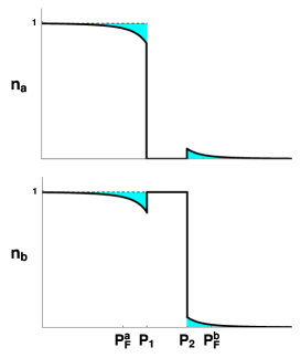
Figure 1: The schematic occupation numbers $n_{a}$ and $n_{b}$ as functions of momentum. $p_{F}^{a}$ and $p_{F}^{b}$ are Fermi momenta of species $a$ and $b$, and $p_{1}$ and $p_{2}$ are the two roots of the dispersion equation $\omega_{-}({\bf p})=0$. The pairing state is breached by the normal fermion liquid state in the region $p_{1}<p<p_{2}$.

IV.2 Spin Susceptibility

We take $g_{a}=g_{b}=1$ for simplicity. While the magnetic moment ${\cal M}$ disappears automatically for normal superconductor, it is no longer zero in the breached pairing superconductor,

$${\cal M}=\mu_{0}(n_{b}-n_{a})=\mu_{0}\frac{p_{2}^{3}-p_{1}^{3}}{6\pi^{2}}\ .$$ (73)

The physical picture is clear: while the paired fermions in the region $p<p_{1}$ and $p>p_{2}$ have no contribution to the magnetic moment, the unpaired fermions in the region $p_{1}<p<p_{2}$ do contribute to ${\cal M}$.

The spin susceptibility in this case is reduced from (62) to

$$\chi=-\mu_{0}^{2}\int_{0}^{\infty}dp\frac{p^{2}}{2\pi^{2}}\left(f^{\prime}(\epsilon_{\Delta}-\delta\mu)+f^{\prime}(\epsilon_{\Delta}+\delta\mu)\right).$$ (74)

At zero temperature, it is nonzero only in the breached pairing state characterized by $\Delta<\delta\mu$,

$$\chi=\frac{\mu_{0}^{2}m}{2\pi^{2}}\frac{\delta\mu}{\sqrt{\delta\mu^{2}-\Delta^{2}}}(p_{1}+p_{2})\ .$$ (75)

From the comparison with the Pauli susceptibility $\chi_{P}$, we have the relation

$${\chi\over\chi_{P}}\sim{\delta\mu\over\sqrt{\delta\mu^{2}-\Delta^{2}}}\ .$$ (76)

V Both Chemical Potential Difference and Mass Difference

We now consider the magnetization property of the superconductor with both chemical potential difference and mass difference between the paired fermions. To simplify the calculation, we still take $Q_{a}=Q_{b}=1$ and $g_{a}=g_{b}=1$. From the dispersion relations

$$\omega_{\pm}(\vec{\bf p})={p^{2}\over 2m_{A}}+\delta\mu\pm\sqrt{\left({p^{2}\over 2m_{S}}-\bar{\mu}\right)^{2}+\Delta^{2}}$$ (77)

with the reduced masses $m_{A}={2m_{a}m_{b}\over m_{b}-m_{a}}$ and $m_{S}={2m_{a}m_{b}\over m_{a}+m_{b}}$, the condition for the system to be in breached pairing state is

$$\Delta<\Delta_{c}=\frac{|m_{b}\mu_{b}-m_{a}\mu_{a}|}{2\sqrt{m_{a}m_{b}}}={|\lambda\mu_{b}-\mu_{a}|\over 2\sqrt{\lambda}}\ ,$$ (78)

where $\lambda=m_{b}/m_{a}$ is the mass ratio, and the corresponding region of breached pairing is located at $p_{1}<p<p_{2}$ in momentum space with

$$p_{1}=\sqrt{m_{a}\left[(\mu_{a}+\lambda\mu_{b})-\sqrt{(\mu_{a}-\lambda\mu_{b})^{2}-4\lambda\Delta^{2}}\right]}\ ,$$

$$p_{2}=\sqrt{m_{a}\left[(\mu_{a}+\lambda\mu_{b})+\sqrt{(\mu_{a}-\lambda\mu_{b})^{2}-4\lambda\Delta^{2}}\right]}\ .$$ (79)

V.1 Meissner Effect

We now calculate analytically the Meissner mass squared at zero temperature. When there is no breached pairing, we have from the general expressions (III.1) to (55),

$$M^{2}=\frac{(\lambda+1)ne^{2}}{2\lambda m_{a}}-\frac{(\lambda-1)^{2}e^{2}}{\lambda^{2}m_{a}^{2}}\int_{0}^{\infty}dp\frac{p^{4}}{6\pi^{2}}\frac{u_{p}^{2}v_{p}^{2}}{\epsilon_{\Delta}}\ .$$ (80)

In the state with breached pairing, taking into account the relation

$${\partial\omega_{-}(p)\over\partial p}=p\left({u_{p}^{2}\over m_{b}}-{v_{p}^{2}\over m_{a}}\right)={p\over\lambda m_{a}}\left(u_{p}^{2}-\lambda v_{p}^{2}\right)$$ (81)

for the integrated function with $f^{\prime}(\omega_{-})$ in (55), the total Meissner mass squared in the breached pairing superconductor can be written as

$$M^{2} = \frac{e^{2}}{6\lambda m_{a}\pi^{2}}\Bigg{[}p_{1}^{3}\left(\lambda-\frac{\left[1+(\lambda-1)v_{1}^{2}\right]^{2}}{|1-(\lambda+1)v_{1}^{2}|}\right)+p_{2}^{3}\left(1-\frac{\left[1+(\lambda-1)v_{2}^{2}\right]^{2}}{|1-(\lambda+1)v_{2}^{2}|}\right)$$ (82)

$$- 3(\lambda+1)\left(\int_{0}^{p_{1}}dpp^{2}u_{p}^{2}-\int_{p_{2}}^{\infty}dpp^{2}v_{p}^{2}\right)-2(\lambda-1)\Bigg{(}\int_{0}^{p_{1}}dpp^{2}\frac{\epsilon_{A}-\delta\mu}{\epsilon_{\Delta}}u_{p}^{2}v_{p}^{2}+\int_{p_{2}}^{\infty}dpp^{2}\frac{\epsilon_{A}-\delta\mu}{\epsilon_{\Delta}}u_{p}^{2}v_{p}^{2}\Bigg{)}\Bigg{]}$$

with the shorthand notations $v_{1}^{2}=v_{p_{1}}^{2}$ and $v_{2}^{2}=v_{p_{2}}^{2}$.

It is easy to check that for $\lambda=1$, we recover the result obtained in Section IV for the case with only chemical potential difference. For $\lambda>1$, we again take the approximation of neglecting the integration terms in (82). Considering the relation

$$1-{\left(1+(\lambda-1)v_{2}^{2}\right)^{2}\over|1-(\lambda+1)v_{2}^{2}|}\leq 0$$ (83)

for any $\lambda$, the sign of $M^{2}$ depends on the quantity

$$\beta(\lambda,v_{1}^{2})=\lambda-{\left(1+(\lambda-1)v_{1}^{2}\right)^{2}\over|1-(\lambda+1)v_{1}^{2}|}\ .$$ (84)

Fig.2 shows $\beta$ as a function of $v_{1}^{2}$ at $\lambda=2$ and $\lambda=10$. Taking into account the condition $v_{1}^{2}=n_{a}(p_{1})=n_{b}(p_{1})>1/2$, we focus on the behavior of $\beta$ in the region of $v_{1}^{2}>1/2$. At $\lambda=2$, $\beta$ is negative in this region and results in negative Meissner mass squared and paramagnetism of the system, which is continued with the conclusion in Section IV. However, at $\lambda=10$, $\beta$ becomes positive in the interesting region, the Meissner mass squared tends to be positive and the system tends to be diamagnetism. In fact, for very large $\lambda$, $v_{2}^{2}$ becomes extremely smallcaldas , and $1-\left(1+(\lambda-1)v_{2}^{2}\right)^{2}/|1-(\lambda+1)v_{2}^{2}|\simeq 0$, the system contains approximately the diamagnetic term only.

Figure 2: The parameter $\beta$ as a function of $v_{1}^{2}$. The dashed and solid lines correspond to $\lambda=2$ and $\lambda=10$, respectively.

V.2 Spin Susceptibility

In the case with both chemical potential difference and mass difference, the magnetic moment ${\cal M}$ in breached pairing state takes still the form of (73), but $p_{1}$ and $p_{2}$ determined by the dispersion relation $\omega_{-}(p)=0$ are shown in (V). As for the spin susceptibility $\chi$, its general expression at finite temperature is still (74). At zero temperature, it is reduced to

$$\chi=\frac{\lambda m_{a}\mu_{0}^{2}}{2\pi^{2}}\left(\frac{p_{1}}{|u_{1}^{2}-\lambda v_{1}^{2}|}+\frac{p_{2}}{|u_{2}^{2}-\lambda v_{2}^{2}|}\right)\ .$$ (85)

VI Extension to Relativistic Systems

We have investigated the Meissner effect and spin susceptibility in an asymmetric system of two kinds of fermions with different chemical potentials, masses, charges, and magnetic moments in nonrelativistic case. We found that the magnetization property of breached pairing superconductor is very different from that of BCS superconductor, and the system tends to be more paramagnetic. What is the situation in relativistic case? Are these exotic phenomena just a consequence of nonrelativistic kinematics? In this section, we extend our discussion to relativistic systems, which is relevant for the study of color superconductivity at high baryon densityhuang ; shovkovy ; huang2 ; alford3 ; huang3 ; huang4 . We will see that there is still paramagnetic Meissner effect in breached pairing state in relativistic superconductors.

VI.1 Without Dirac Structure

As a naive calculation, we first neglect the antiparticles and take the same Lagrangian density (42). The relativistic effect is only reflected in the fermion energies $\epsilon_{p}^{a}=\sqrt{p^{2}+m_{a}^{2}}-\mu_{a}$, $\epsilon_{p}^{b}=\sqrt{p^{2}+m_{b}^{2}}-\mu_{b}$. The formulas for Meissner mass squared and spin susceptibility in Section III still hold if we replace $m_{i}(i=a,b)$ there by $\sqrt{p^{2}+m_{i}^{2}}$. As an example, we list here the diamagnetic and paramagnetic parts of the Meissner mass squared in the case with only chemical potential difference between the two species,

$$M^{2}_{D} = {n_{r}e^{2}\over m}\ ,$$ (86)

$$M_{P}^{2} = {e^{2}\over 6\pi^{2}}\int_{0}^{\infty}dp\frac{p^{4}}{p^{2}+m^{2}}\left[f^{\prime}\left(\epsilon_{\Delta}-\delta\mu\right)+f^{\prime}\left(\epsilon_{\Delta}+\delta\mu\right)\right]$$

with the relativistic fermion density

$$n_{r}=\int_{0}^{\infty}\frac{d^{3}\vec{\bf p}}{(2\pi)^{3}}\frac{m}{\sqrt{p^{2}+m^{2}}}\left[n_{a}(p)+n_{b}(p)\right]\ .$$ (87)

In ultra relativistic limit $m\rightarrow 0$ and at zero temperature, they can be evaluated as

$$M^{2}_{D} \simeq \frac{e^{2}\bar{\mu}^{2}}{\pi^{2}}\left(1+\frac{\delta\mu^{2}-\Delta^{2}}{\bar{\mu}^{2}}\right)\ ,$$ (88)

$$M^{2}_{P} = -\frac{e^{2}\bar{\mu}^{2}}{3\pi^{2}}\frac{\delta\mu}{\sqrt{\delta\mu^{2}-\Delta^{2}}}\left(1+\frac{\delta\mu^{2}-\Delta^{2}}{\bar{\mu}^{2}}\right)\theta(\delta\mu-\Delta)\ ,$$

where in the calculation of $M_{D}^{2}$ we have taken again the approximation used in deriving (72). The paramagnetic part is automatically zero in normal superconductor with $\Delta>\delta\mu$, but negative in breached pairing superconductor with $\Delta<\delta\mu$. Putting the two terms together, the total Meissner mass squared can be expressed as

$$M^{2}=\frac{e^{2}\bar{\mu}^{2}}{3\pi^{2}}\left(1+\frac{\delta\mu^{2}-\Delta^{2}}{\bar{\mu}^{2}}\right)\left(3-\frac{\delta\mu\theta(\delta\mu-\Delta)}{\sqrt{\delta\mu^{2}-\Delta^{2}}}\right)\ .$$ (89)

It is negative in the case of $\Delta<\sqrt{8/9}\delta\mu<\delta\mu$. Therefore, a relativistic breached pairing superconductor is also paramagnetic.

VI.2 With Dirac Structure

We study now a more realistic relativistic model containing two kinds of fermions. The Lagrangian of the system is defined as

$${\cal L}=\sum_{\alpha=a,b}\bar{\psi}_{\alpha}\left(i\gamma^{\mu}\partial_{\mu}-m_{\alpha}+\mu_{\alpha}\gamma_{0}\right)\psi_{\alpha}+g\sum_{\alpha,\beta=a,b}\left(\bar{\psi}^{C}_{\alpha}i\gamma_{5}\tau_{1}^{\alpha\beta}\psi_{\beta}\right)\sum_{\alpha,\beta=a,b}\left(\bar{\psi}_{\alpha}i\gamma_{5}\tau_{1}^{\alpha\beta}\psi^{C}_{\beta}\right)\ ,$$ (90)

where $\gamma^{\mu}=(\gamma^{0},\gamma^{1},\gamma^{2},\gamma^{3})=(\beta,\beta\alpha^{1},\beta\alpha^{2},\beta\alpha^{3})$ and $\gamma^{5}=i\gamma^{0}\gamma^{1}\gamma^{2}\gamma^{3}$ are Dirac matrices with $\beta$ and $\alpha^{i}$ being anticommuting matrices, $\beta^{2}=\alpha_{i}^{2}=1,\{\alpha_{i},\alpha_{j}\}=0$ for $i\neq j$, and $\{\alpha_{i},\beta\}=0$, their covariant counterparts $\gamma_{\mu}$ and $\gamma_{5}$ are defined as $\gamma_{\mu}=(\gamma^{0},-\gamma^{1},-\gamma^{2},-\gamma^{3})$ and $\gamma_{5}=\gamma^{5}$, $\psi$ and $\bar{\psi}$ are Dirac spinors, $\psi^{C}=C\bar{\psi}^{T}$ and $\bar{\psi}^{C}=\psi^{T}C$ are charge-conjugate spinors, $C=i\gamma^{2}\gamma^{0}$ is the charge conjugation matrix, the superscript $T$ denotes transposition operation, and $\tau_{1}$ is the first Pauli matrix with the elements $\tau_{1}^{aa}=\tau_{1}^{bb}=0$ and $\tau_{1}^{ab}=\tau_{1}^{ba}=1$.

For convenience we define the Nambu-Gorkov spinors

$$\Psi=\left(\begin{array}[]{c}\psi_{a}\\ \psi^{C}_{b}\\ \psi_{b}\\ \psi^{C}_{a}\end{array}\right)\ ,\ \ \ \bar{\Psi}=\left(\begin{array}[]{cccc}\bar{\psi}_{a}&\bar{\psi}^{C}_{b}&\bar{\psi}_{b}&\bar{\psi}^{C}_{a}\end{array}\right)\ .$$ (91)

Introducing the order parameter

$$\Delta=-2g\sum_{\alpha,\beta=a,b}\Big{\langle}\bar{\psi}^{C}_{\alpha}i\gamma_{5}\tau_{\alpha\beta}\psi_{\beta}\Big{\rangle}\ ,$$ (92)

and taking it to be real, the thermodynamic potential of the system in mean field approximation is still in the form of (9) with the propagator matrix defined in the 4-dimensional Nambu-Gorkov space,

$${\cal G}^{-1}=\left(\begin{array}[]{cccc}[{\cal G}_{0}^{+}]_{a}^{-1}&i\gamma_{5}\Delta&0&0\\ i\gamma_{5}\Delta&[{\cal G}_{0}^{-}]_{b}^{-1}&0&0\\ 0&0&[{\cal G}_{0}^{+}]_{b}^{-1}&i\gamma_{5}\Delta\\ 0&0&i\gamma_{5}\Delta&[{\cal G}_{0}^{-}]_{a}^{-1}\end{array}\right)\ ,$$ (97)

where ${\cal G}_{0}$ is the free propagator,

$$[{\cal G}_{0}^{\pm}]_{\alpha}^{-1}=i\omega_{n}\gamma_{0}-\vec{\gamma}\cdot\vec{\bf p}-m_{\alpha}\pm\mu_{\alpha}\gamma_{0}\$$ (98)

with the vector matrix $\vec{\gamma}=(\gamma^{1},\gamma^{2},\gamma^{3})$.

Assuming that the fermion field $\psi_{\alpha}$ with charge $e$ can couple to some $U(1)$ gauge potential $A_{\mu}$, the Meissner mass squared can be extracted from the expansion of the thermodynamic potential in powers of the external magnetic potential $\vec{\bf A}$. By separating the $\vec{\bf A}$-dependent propagator (97) into two terms,

$${\cal G}_{A}^{-1}(i\omega_{n},p)={\cal G}^{-1}+e\Sigma\vec{\gamma}\cdot\vec{\bf A}\ ,$$ (99)

with the self-energy matrix $\Sigma$ defined by

$$\Sigma=\left(\begin{array}[]{cccc}1&0&0&0\\ 0&-1&0&0\\ 0&0&1&0\\ 0&0&0&-1\end{array}\right)\ ,$$ (100)

and taking the coefficient of the quadratic term in $\vec{\bf A}$ of $\Omega(\vec{\bf A})$, the Meissner mass squared can be evaluated as

$$M^{2}=e^{2}T\sum_{n}\int\frac{d^{3}\vec{\bf p}}{(2\pi)^{3}}\sum_{i=1}^{3}Tr\Big{[}{\cal G}_{11}\gamma^{i}{\cal G}_{11}\gamma^{i}+{\cal G}_{22}\gamma^{i}{\cal G}_{22}\gamma^{i}+{\cal G}_{33}\gamma^{i}{\cal G}_{33}\gamma^{i}+{\cal G}_{44}\gamma^{i}{\cal G}_{44}\gamma^{i}-2{\cal G}_{12}\gamma^{i}{\cal G}_{21}\gamma^{i}-2{\cal G}_{34}\gamma^{i}{\cal G}_{43}\gamma^{i}\Big{]}\ .$$ (101)

In the case of $m_{a}=m_{b}$, it is straightforward to write down explicitly the propagator matrix elements ${\cal G}_{ij}$, by employing the method used in huang5 ; he ,

$${\cal G}_{11}(i\omega_{n},p) = {i\omega_{n}+\epsilon_{p}^{-}-\delta\mu\over(i\omega_{n}-\delta\mu)^{2}-(\epsilon_{\Delta}^{-})^{2}}\Lambda_{+}\gamma_{0}+{i\omega_{n}-\epsilon_{p}^{+}-\delta\mu\over(i\omega_{n}-\delta\mu)^{2}-(\epsilon_{\Delta}^{+})^{2}}\Lambda_{-}\gamma_{0}\ ,$$

$${\cal G}_{22}(i\omega_{n},p) = {i\omega_{n}-\epsilon_{p}^{-}-\delta\mu\over(i\omega_{n}-\delta\mu)^{2}-(\epsilon_{\Delta}^{-})^{2}}\Lambda_{-}\gamma_{0}+{i\omega_{n}+\epsilon_{p}^{+}-\delta\mu\over(i\omega_{n}-\delta\mu)^{2}-(\epsilon_{\Delta}^{+})^{2}}\Lambda_{+}\gamma_{0}\ ,$$

$${\cal G}_{12}(i\omega_{n},p) = {i\Delta\over(i\omega_{n}-\delta\mu)^{2}-(\epsilon_{\Delta}^{-})^{2}}\Lambda_{-}\gamma_{5}+{i\Delta\over(i\omega_{n}-\delta\mu)^{2}-(\epsilon_{\Delta}^{+})^{2}}\Lambda_{+}\gamma_{5}\ ,$$

$${\cal G}_{21}(i\omega_{n},p) = {i\Delta\over(i\omega_{n}-\delta\mu)^{2}-(\epsilon_{\Delta}^{-})^{2}}\Lambda_{+}\gamma_{5}+{i\Delta\over(i\omega_{n}-\delta\mu)^{2}-(\epsilon_{\Delta}^{+})^{2}}\Lambda_{-}\gamma_{5}\ ,$$

$${\cal G}_{33}(i\omega_{n},p) = {i\omega_{n}+\epsilon_{p}^{-}+\delta\mu\over(i\omega_{n}+\delta\mu)^{2}-(\epsilon_{\Delta}^{-})^{2}}\Lambda_{+}\gamma_{0}+{i\omega_{n}-\epsilon_{p}^{+}+\delta\mu\over(i\omega_{n}+\delta\mu)^{2}-(\epsilon_{\Delta}^{+})^{2}}\Lambda_{-}\gamma_{0}\ ,$$

$${\cal G}_{44}(i\omega_{n},p) = {i\omega_{n}-\epsilon_{p}^{-}+\delta\mu\over(i\omega_{n}+\delta\mu)^{2}-(\epsilon_{\Delta}^{-})^{2}}\Lambda_{-}\gamma_{0}+{i\omega_{n}+\epsilon_{p}^{+}+\delta\mu\over(i\omega_{n}+\delta\mu)^{2}-(\epsilon_{\Delta}^{+})^{2}}\Lambda_{+}\gamma_{0}\ ,$$

$${\cal G}_{34}(i\omega_{n},p) = {i\Delta\over(i\omega_{n}+\delta\mu)^{2}-(\epsilon_{\Delta}^{-})^{2}}\Lambda_{-}\gamma_{5}+{i\Delta\over(i\omega_{n}+\delta\mu)^{2}-(\epsilon_{\Delta}^{+})^{2}}\Lambda_{+}\gamma_{5}\ ,$$

$${\cal G}_{43}(i\omega_{n},p) = {i\Delta\over(i\omega_{n}+\delta\mu)^{2}-(\epsilon_{\Delta}^{-})^{2}}\Lambda_{+}\gamma_{5}+{i\Delta\over(i\omega_{n}+\delta\mu)^{2}-(\epsilon_{\Delta}^{+})^{2}}\Lambda_{-}\gamma_{5},$$ (102)

with the quasi-particle energies

$$\epsilon_{p}^{\pm}=\sqrt{p^{2}+m^{2}}\pm\bar{\mu}\ ,\ \ \ \epsilon_{\Delta}^{\pm}=\sqrt{(\epsilon_{p}^{\pm})^{2}+\Delta^{2}}\ ,$$ (103)

and the energy projectors

$$\Lambda_{\pm}={1\over 2}\left(1\pm{\gamma_{0}\vec{\gamma}\cdot\vec{\bf p}\over\sqrt{p^{2}+m^{2}}}\right)\ .$$ (104)

It is easy to see that in the ultra relativistic limit $m\rightarrow 0$, the expression (101) is just the same as the 8th gluon’s Meissner mass squared in the two flavor gapless color superconductorhuang3 ; huang4 , namely,

$$M^{2}\approx\frac{2e^{2}\bar{\mu}^{2}}{3\pi^{2}}\left[1-\frac{\delta\mu\theta(\delta\mu-\Delta)}{\sqrt{\delta\mu^{2}-\Delta^{2}}}\right]\ .$$ (105)

Since we did not consider here the non-Abelian structure of the color superconductivity, the negative Meissner mass squared for the 8th gluon is just a reflection of the breached pairing mechanism.

VII Summary

We have investigated the relation between the pairing mechanism and magnetization property of superconductivity in an asymmetric two-component fermion system coupled to a magnetic potential. In the frame of field theory approach, we derived the dependence of the Meissner mass squared, magnetic moment, and spin susceptibility of the system on the chemical potential difference, mass difference, charge difference, and magnetic moment difference between the two kinds of fermions. Compared with the superconductor formed in a symmetric system where the Meissner mass squared is globally diamagnetic, there is no magnetic moment, and the spin susceptibility disappears at zero temperature, we found the following new magnetization properties for the asymmetric system with mismatched Fermi surfaces between the paired fermions:

1) The asymmetry leads to a new paramagnetic term in the Meissner mass squared and a new term in the spin susceptibility, and the magnetic moment is no longer zero in asymmetric systems. Note that the new terms and the finite magnetic moment do not depend on the pairing mechanism, they are only the consequence of asymmetry between the two species.

2) At the turning point from BCS to breached pairing state, the Meissner mass squared and spin susceptibility are divergent at zero temperature.

3) In the breached pairing state induced by chemical potential difference between the two paired fermions, the Meissner mass squared is paramagnetic at zero temperature.

4) In the breached pairing state with not only chemical potential difference but also mass difference between the two kinds of fermions, the system at zero temperature is paramagnetic at small mass ratio and tends to be diamagnetic when the ratio is large enough.

While the paramagnetic Meissner effect and finite spin susceptibility discussed above are interesting, how to understand them correctly and their reflection on physically observable quantities are not clear. By comparing the BP and LOFF statesgiannakis ; giannakis2 ; dukelsy , the paramagnetic Meissner effect might be a signal of instability of the BP stategiannakis ; giannakis2 . The thermodynamic potential $\Omega(\vec{\bf Q})$ of a LOFF state with a nonzero momentum $2\vec{\bf Q}$ of the Cooper pair can be obtained by replacing the magnetic potential $e\vec{\bf A}$ in the thermodynamic potential $\Omega(\vec{\bf A})$ derived above by the momentum $\vec{\bf Q}$. If the uniform BP state is the ground state, the thermodynamic potential must be the minimum at $\vec{\bf Q}=0$, namely, $\partial\Omega/\partial Q_{i}=0$ and $\kappa=\partial^{2}\Omega/\partial Q^{2}>0$ at $\vec{\bf Q}=0$. Through the obvious relation $M^{2}=e^{2}\kappa$, negative Meissner mass squared leads automatically to negative $\kappa$. Therefore, the paramagnetic Meissner effect may be a signal that the LOFF state is more favored than the BP state. However, the above argument is obtained from the study for systems with fixed chemical potentials, it is not clear if it is still true for systems with fixed number densities of the two species. As we know, the existence of the LOFF phase in conventional superconductors has still not been convincingly demonstrated in any material. If the above argument is true, the LOFF state might be observed in trapped atomic fermion systemsmizhushima ; yang . Our research in this direction is in progress.

Acknowledgments: We thank Prof. Hai-cang Ren and Dr. Mei Huang for stimulating discussions and comments. The work was supported in part by the grants NSFC10428510, 10435080, 10447122 and SRFDP20040003103.

Appendix A Fermion Frequency Summations

We calculate in this Appendix the fermion frequency summations $T\sum_{n}{\cal G}_{11}{\cal G}_{11}$, $T\sum_{n}{\cal G}_{22}{\cal G}_{22}$, and $T\sum_{n}{\cal G}_{12}{\cal G}_{21}$ in the Meissner mass squared and spin susceptibility in Sections III, IV and V. From the decomposition of these summations,

$$T\sum_{n}{\cal G}_{11}{\cal G}_{11} = T\sum_{n}\frac{(i\omega_{n}-\epsilon_{A}+\epsilon_{S})^{2}}{[(i\omega_{n}-\epsilon_{A})^{2}-\epsilon_{\Delta}^{2}]^{2}}=A+(\epsilon_{\Delta}+\epsilon_{S})^{2}B+2\epsilon_{S}C\ ,$$

$$T\sum_{n}{\cal G}_{22}{\cal G}_{22} = T\sum_{n}\frac{(i\omega_{n}-\epsilon_{A}-\epsilon_{S})^{2}}{[(i\omega_{n}-\epsilon_{A})^{2}-\epsilon_{\Delta}^{2}]^{2}}=A+(\epsilon_{\Delta}-\epsilon_{S})^{2}B-2\epsilon_{S}C\ ,$$

$$T\sum_{n}{\cal G}_{12}{\cal G}_{21} = T\sum_{n}\frac{\Delta^{2}}{[(i\omega_{n}-\epsilon_{A})^{2}-\epsilon_{\Delta}^{2}]^{2}}=\Delta^{2}B\ ,$$

with the definitions

$$A = T\sum_{n}\frac{1}{(i\omega_{n}-\epsilon_{A})^{2}-\epsilon_{\Delta}^{2}}\ ,\ \ \ B=T\sum_{n}\frac{1}{[(i\omega_{n}-\epsilon_{A})^{2}-\epsilon_{\Delta}^{2}]^{2}}\ ,$$

$$C = T\sum_{n}\frac{1}{(i\omega_{n}-\epsilon_{A}+\epsilon_{\Delta})^{2}(i\omega_{n}-\epsilon_{A}-\epsilon_{\Delta})}\ ,$$

we need to complete the summations $A,B$ and $C$ only,

$$A = \frac{f(-\omega_{-})+f(\omega_{+})-1}{2\epsilon_{\Delta}}\ ,\ \ \ B=\frac{1}{2\epsilon_{\Delta}}\frac{\partial}{\partial\epsilon_{\Delta}}\left[\frac{f(-\omega_{-})+f(\omega_{+})-1}{2\epsilon_{\Delta}}\right]\ ,$$

$$C = \frac{f(-\omega_{-})+f(\omega_{+})-1}{4\epsilon_{\Delta}^{2}}-\frac{1}{2\epsilon_{\Delta}}\frac{\partial f(-\omega_{-})}{\partial\epsilon_{\Delta}}\ .$$

Defining the function $f^{\prime}(x)=\partial f(x)/\partial x$, we can express the summations we need as

$$T\sum_{n}{\cal G}_{11}{\cal G}_{11} = u_{p}^{2}v_{p}^{2}\frac{f(\omega_{+})-f(\omega_{-})}{\epsilon_{\Delta}}+v_{p}^{4}f^{\prime}(\omega_{-})+u_{p}^{4}f^{\prime}(\omega_{+})\ ,$$

$$T\sum_{n}{\cal G}_{22}{\cal G}_{22} = u_{p}^{2}v_{p}^{2}\frac{f(\omega_{+})-f(\omega_{-})}{\epsilon_{\Delta}}+u_{p}^{4}f^{\prime}(\omega_{-})+v_{p}^{4}f^{\prime}(\omega_{+})\ ,$$

$$T\sum_{n}{\cal G}_{12}{\cal G}_{21} = -u_{p}^{2}v_{p}^{2}\frac{f(\omega_{+})-f(\omega_{-})}{\epsilon_{\Delta}}+u_{p}^{2}v_{p}^{2}\left[f^{\prime}(\omega_{-})+f^{\prime}(\omega_{+})\right]\ ,$$

where the energies $\epsilon_{A},\epsilon_{S},\epsilon_{\Delta}$, the dispersion relations $\omega_{+},\omega_{-}$, and the functions $u_{p}^{2},v_{p}^{2}$ are defined in Section III.

References

- (1) See, for instance, A.L.Fetter and J.D.Walecka, Quantum Theory of Many-Particle Systems, McGraw-Hill, INC. 1971.
- (2) See, for instance, S.Weinberg, The Quantum Theory of Fields, Cambridge University Press, 1996.
- (3) See, for reviews, K.Rajagopal and F.Wilczek, hep-ph/0011333; M.Alford, Ann. Rev. Nucl. Part. Sci. 51, 131(2001); T.Schäfer, hep-ph/0304281; H.Ren, hep-ph/0404074; M.Huang, hep-ph/0409167; M.Buballa, Phys. Rept. 407, 205(2005).
- (4) G.Sarma, J.Phys.Chem.Solid 24,1029(1963).
- (5) P.Fulde and R.A.Ferrell,Phys. Rev A135,550(1964).
- (6) A.I.Larkin and Yu.N.Ovchinnikov, Sov.Phys. JETP 20(1965).
- (7) S.Takada and T.Izuyama, Prog.Theor.Phys.41,635(1969)
- (8) W.V.Liu and F.Wilczek, Phys. Rev. Lett.90, 047002(2003).
- (9) H.H.Suhl,B.T.Matthias and L.R.Walker, Phys.Rev.Lett.3,552(1959).
- (10) J.Kondo, Prog.Theor.Phys.29,1(1963).
- (11) J.I.Cirac and P.Zoller, Physics Today 57,38(2004).
- (12) H.Caldas, Phys. Rev. A69, 063602(2004).
- (13) A.Sedrakian and U.Lombardo, Phys. Rev. Lett. 84, 602(2000).
- (14) T.Schäfer and F.Wilczek, Phys. Rev. D60, 074014 (1999).
- (15) M.Alford, J.Berbges, and K.Rajagopal, Nucl. Phys. B558, 219 (1999).
- (16) K.Rajagopal and F.Wilczek, Phys. Rev. Lett. 86, 3492 (2001).
- (17) A.W.Steiner, S.Reddy, and M.Prakash, Phys. Rev. D66, 094007(2002).
- (18) M.Alford and K.Rajagopal, JHEP 06, 031(2002).
- (19) M.Huang, P.Zhuang, and W.Chao, Phys. Rev. D67, 065015(2003).
- (20) H.Abuki, M.Kitazawa, T.Kunihiro, Phys. Lett. B615, 102(2005).
- (21) S.B.Ruster, V.Werth, M.Buballa et al., Phys. Rev. D72, 034004 (2005).
- (22) D.Blaschke, S.Fredriksson, H.Grigorian, et al., hep-ph/0503194.
- (23) I.Shovkovy and M.Huang, Phys. Lett. B564 205(2003).
- (24) M.Huang and I.Shovkovy, Nucl. Phys. A729, 835(2003).
- (25) M.Alford, C.Kouvaris and K. Rajagopal, Phys. Rev. Lett. 92, 222001(2004).
- (26) S.Wu and S.Yip, Phys. Rev. A67, 053603(2003).
- (27) W.V.Liu and F.Wilczek, cond-mat/0304632.
- (28) M.M.Forbes, E.Gubankova, W. Vincent Liu, F.Wilczek, Phys. Rev. Lett.94, 017001(2005).
- (29) J.Liao and P.Zhuang, Phys. Rev. D68, 114016(2003).
- (30) M.Huang and I.Shovkovy, Phys.Rev. D70, R051501(2004).
- (31) M.Huang and I.Shovkovy, Phys. Rev. D70, 094030(2004).
- (32) P.Svedlindh, K.Niskanen, P.Norling, et al., Physica C 162-164,1365(1989).
- (33) W.Braunisch, N.Knauf, V.Kataev, et al., Phys.Rev.Lett.68,1908(1992); W.Braunisch, N.Knauf, G.Bauer, et al., Phys.Rev.B.48,4030(1993).
- (34) D.J.Thompson, M.S.M.Minhaj, L.E.Wenger and J.T.Chen, Phys.Rev.Lett.75,529(1995).
- (35) P.Kosti, B.Veal, A.P.Paulikas, et al., Phys.Rev.B.53,791(1996); Phys.Rev.B.55,14649(1997).
- (36) F.M.Araujo-Moreira, P.Barbara, A.B.Cawthorne and C.J.Lobb, Phys.Rev.Lett.78,4625(1997).
- (37) P.Barbara, F.M.Araujo-Moreira, A.B.Cawthorne and C.J.Lobb, Phys.Rev.B.60,7489(1999).
- (38) M.Sigrist and T.M.Rice, Phys.Soc.Jpn.61,4283(1992).
- (39) K.M.Lang, V.Madhavan, J.E.Hoffman et al., Nature(London) 415,412(2002).
- (40) K.Fukushima, hep-ph/0506080.
- (41) D.K.Hong, ep-ph/0506097.
- (42) M.Huang,P.Zhuang and W.Chao, Phys. Rev.D65, 076012(2002).
- (43) L.He, M.Jin and P.Zhuang, Phys.Rev. D71, 116001(2005).
- (44) I.Giannakis and H.Ren, Phys. Lett. B611, 137(2005).
- (45) I.Giannakis and H.Ren, Nucl. Phys. B723, 255(2005).
- (46) J.Dukelsy, G.Ortiz, and S.M.A.Rombouts, cond-mat/0510635.
- (47) T.Mizhushima, K.Machida, and M.Ichioka, Phys. Rev. Lett. 94, 060404 (2005).
- (48) Kun Yang, Phys. Rev. Lett. 95, 218903 (2005).