Hadronic decays of the tau lepton : $\tau^{-}\rightarrow\left(\pi\pi\pi\right)^{-}\nu_{\tau}$ within Resonance Chiral Theory

Abstract

$\tau$ decays into hadrons foresee the study of the hadronization of vector and axial-vector QCD currents, yielding relevant information on the dynamics of the resonances entering into the processes. We analyse $\tau\rightarrow\pi\pi\pi\nu_{\tau}$ decays within the framework of the Resonance Chiral Theory, comparing this theoretical scheme with the experimental data, namely ALEPH spectral function and branching ratio. Hence we get values for the mass and on-shell width of the $a_{1}(1260)$ resonance, and provide the structure functions that have been measured by OPAL and CLEO-II.

1 Introduction

The implementation of Quantum Chromodynamics (QCD) in the energy region populated by light-flavoured resonances ($M_{\rho}\stackrel{{\scriptstyle<}}{{{}_{\sim}}}E\stackrel{{\scriptstyle<}}{{{}_{\sim}}}2\;\mbox{GeV}$, being $M_{\rho}$ the mass of the $\rho(770)$) is a demanding task that involves poorly known aspects such as bound and resonant states, duality and hadronization mechanisms. Though ad hoc Breit-Wigner parameterisations have been widely employed in the literature Pich:1989pq ; Achasov:1996gw they are not necessarily consistent with the underlying theory, as they seem to violate the chiral symmetry of massless QCD Portoles:2000sr ; GomezDumm:2003ku .

$\tau$ decays into hadrons allow to study the hadronization properties of vector and axial-vector QCD currents and, accordingly, to determine intrinsic properties of the dynamics generated by resonances Portoles:2004vr . At very low energies, typically $E\ll M_{\rho}$, Chiral Perturbation Theory ($\chi$PT) Weinberg:1978kz is the Effective Field Theory of QCD. Still the $\tau\rightarrow\pi\pi\pi\nu_{\tau}$ decays, through their full energy spectrum, are driven by the $\rho(770)$ and $a_{1}(1260)$ resonances mainly, in an energy region where the invariant hadron momentum approaches the masses of the resonances. Hence $\chi$PT is no longer applicable to the study of the whole spectrum but only to the very low energy domain Colangelo:1996hs . The standard procedure that has been followed Pich:1989pq to deal with these decays has been to modulate the amplitudes with a Breit-Wigner parameterization, fixing the normalization in order to match the leading ${\cal O}(p^{2})$ $\chi$PT. Nevertheless, its deviation of the chiral behaviour at higher orders Portoles:2000sr ; GomezDumm:2003ku could spoil any outcome provided by the analysis of data.

Lately several experiments have collected good quality data on $\tau\rightarrow\pi\pi\pi\nu_{\tau}$, such as branching ratios and spectra Barate:1998uf or structure functions Ackerstaff:1997dv . Their analysis within a model-independent framework is highly desirable if one wishes to collect information on the hadronization of the relevant QCD currents.

2 The Resonance Chiral Theory of QCD

At energies $E\sim M_{\rho}$ the resonance mesons are active degrees of freedom that have to be properly included into the pertinent Lagrangian. The procedure, put forward in Refs. Ecker:1988te ; Ecker:1989yg and known as Resonance Chiral Theory (R$\chi$T), is ruled by the approximate chiral symmetry of QCD, that drives the interaction of Goldstone bosons (the lightest octet of pseudoscalar mesons), and the $SU(3)_{V}$ assignments of the resonance multiplets. This construction is embedded within a comprehensive framework guided by the large number of colours ($N_{C}$) limit of QCD 'tHooft:1974hx . The $1/N_{C}$ expansion tells us that, at leading order, we should only consider the tree level diagrams given by a local Lagrangian with infinite zero-width states in the spectrum. This is precisely the role of R$\chi$T. However in most processes, like hadron tau decays, we need to include finite widths that only appear at next-to-leading order in the large-$N_{C}$ expansion and, moreover, we will only include one multiplet of vector and axial-vector resonances in our theory. Thus, in practice, we have to model this large-$N_{C}$ expansion to some extent.

The final hadron system in the $\tau\rightarrow\pi\pi\pi\nu_{\tau}$ decays spans a wide energy region, namely $3\,m_{\pi}\stackrel{{\scriptstyle<}}{{{}_{\sim}}}E\stackrel{{\scriptstyle<}}{{{}_{\sim}}}M_{\tau}$ that is populated by many resonances. R$\chi$T is the appropriate framework to work with and we consider the Lagrangian GomezDumm:2003ku ; Ecker:1988te  :

$${\cal L}_{\rm R\chi T} = \frac{F^{2}}{4}\langle u_{\mu}u^{\mu}+\chi_{+}\rangle\,+\,\frac{F_{V}}{2\sqrt{2}}\langle V_{\mu\nu}f_{+}^{\mu\nu}\rangle\,+\,i\,\frac{G_{V}}{\sqrt{2}}\langle V_{\mu\nu}u^{\mu}u^{\nu}\rangle\,+\,\frac{F_{A}}{2\sqrt{2}}\langle A_{\mu\nu}f_{-}^{\mu\nu}\rangle\,$$ (1)

$$+\,{\cal L}_{\rm kin}^{\rm V}\,+\,{\cal L}_{\rm kin}^{\rm A}\,+\,\sum_{i=1}^{5}\,\lambda_{i}\,{\cal O}^{i}_{\rm VAP}\,,$$

where all the couplings are real, being $F$ the decay constant of the pion in the chiral limit, and the operators ${\cal O}_{VAP}^{i}$ are given by :

$${\cal O}^{1}_{\rm VAP} = \langle\,[\,V^{\mu\nu}\,,\,A_{\mu\nu}\,]\,\chi_{-}\,\rangle\;\;,$$

$${\cal O}^{2}_{\rm VAP} = i\,\langle\,[\,V^{\mu\nu}\,,\,A_{\nu\alpha}\,]\,h_{\mu}^{\;\alpha}\,\rangle\;\;,$$ (2)

$${\cal O}^{3}_{\rm VAP} = i\,\langle\,[\,\nabla^{\mu}V_{\mu\nu}\,,\,A^{\nu\alpha}\,]\,u_{\alpha}\,\rangle\;\;,$$

$${\cal O}^{4}_{\rm VAP} = i\,\langle\,[\,\nabla^{\alpha}V_{\mu\nu}\,,\,A_{\alpha}^{\;\nu}\,]\,u^{\mu}\,\rangle\;\;,$$

$${\cal O}^{5}_{\rm VAP} = i\,\langle\,[\,\nabla^{\alpha}V_{\mu\nu}\,,\,A^{\mu\nu}\,]\,u_{\alpha}\,\rangle\;\;.$$

The notation is that of Ref. Ecker:1988te . Notice that we are using the antisymmetric tensor formulation to describe the spin $1$ resonances and, consequently, we do not consider the ${\cal O}(p^{4})$ $\chi$PT Lagrangian of Goldstone bosons Ecker:1989yg .

Our Lagrangian theory has eight a priori unknown coupling constants, namely $F_{V}$, $F_{A}$, $G_{V}$ and $\lambda_{i}$, $i=1,...5$. Phenomenology could provide direct information on them; for instance $F_{V}$ could be extracted from the measured $\Gamma(\rho^{0}\rightarrow e^{+}e^{-})$, $G_{V}$ from $\Gamma(\rho^{0}\rightarrow\pi^{+}\pi^{-})$, $F_{A}$ from $\Gamma(a_{1}\rightarrow\pi\gamma)$ and the $\lambda_{i}$ appear in $\Gamma(a_{1}\rightarrow\rho\pi)$ or the $\tau\to\pi\pi\pi\nu_{\tau}$ processes themselves. It is conspicuous, though, that ${\cal L}_{R\chi T}$ is not QCD for arbitrary values of the couplings. Hence if we want to comprehend more about QCD in this non-perturbative regime we should try to learn about the determination of the couplings from the underlying theory Pich:2002xy . On this account we will implement several known features of the strong interaction theory in the following.

The QCD ruled short–distance behaviour of the vector and axial-vector form factors in the large–$N_{C}$ limit (approximated with only one octet of vector resonances) constrains the couplings of ${\cal L}_{\rm R\chi T}$ in Eq. (1), which must satisfy Ecker:1989yg  :

$$1\,-\,\frac{F_{V}\,G_{V}}{F^{2}} = 0\;\;,$$

$$2F_{V}G_{V}\,-\,F_{V}^{2}\, = 0\;\;.$$ (3)

In addition, the first Weinberg sum rule, in the limit where only the lowest narrow resonances contribute to the vector and axial–vector spectral functions, leads to

$$F_{V}^{2}-F_{A}^{2}=F^{2}\;.$$ (4)

In this way all three couplings $F_{V}$, $G_{V}$ and $F_{A}$ can be written in terms of the pion decay constant : $F_{V}=\sqrt{2}F$, $G_{V}=F/\sqrt{2}$ and $F_{A}=F$. These results are well satisfied phenomenologically and we have adopted them. In the next section we will comment on an analogous study of the $\lambda_{i}$ couplings.

3 The axial-vector form factors in $\tau^{-}\rightarrow\left(\pi\pi\pi\right)^{-}\nu_{\tau}$

The decay amplitudes for the $\tau^{-}\rightarrow\pi^{+}\pi^{-}\pi^{-}\nu_{\tau}$ and $\tau^{-}\rightarrow\pi^{-}\pi^{0}\pi^{0}\nu_{\tau}$ processes can be written as

$${\cal M}_{\pm}\,=\,-\,\frac{G_{F}}{\sqrt{2}}\,V_{ud}\,\bar{u}_{\nu_{\tau}}\gamma^{\mu}\,(1-\gamma_{5})u_{\tau}\,T_{\pm\mu}\;,$$ (5)

$$T_{\pm\mu}(p_{1},p_{2},p_{3})\,=\,\langle\pi_{1}(p_{1})\pi_{2}(p_{2})\pi^{\pm}(p_{3})|{\cal A}_{\mu}|0\rangle\,,$$ (6)

as in the isospin limit there is no contribution of the vector current to these processes. In $T_{\pm\mu}(p_{1},p_{2},p_{3})$ the $\pi^{+}$ is the one in $\tau^{-}\to\pi^{+}\pi^{-}\pi^{-}\nu_{\tau}$ and $\pi^{-}$ that in $\tau^{-}\to\pi^{-}\pi^{0}\pi^{0}\nu_{\tau}$. The hadronic tensor can be written in terms of three form factors, $F_{1}$, $F_{2}$ and $F_{P}$, as Kuhn:1992nz  :

$$T^{\mu}\;=\;V_{1}^{\mu}\,F_{1}\,+\,V_{2}^{\mu}\,F_{2}\,+\,Q^{\mu}\,F_{P}\;\;,$$ (7)

where

$$V_{1}^{\mu} = \left(\,g^{\mu\nu}\,-\,\frac{Q^{\mu}Q^{\nu}}{Q^{2}}\,\right)\,(\,p_{1}-p_{3}\,)_{\nu}\;\;,$$

$$V_{2}^{\mu} = \left(\,g^{\mu\nu}\,-\,\frac{Q^{\mu}Q^{\nu}}{Q^{2}}\,\right)\,(\,p_{2}-p_{3}\,)_{\nu}\;\;,$$

$$Q^{\mu} = p_{1}^{\mu}+p_{2}^{\mu}+p_{3}^{\mu}\;\;.$$ (8)

The form factors $F_{1}$ and $F_{2}$ have a transverse structure in the total hadron momenta $Q_{\mu}$ and drive a $J^{P}=1^{+}$ transition. Bose symmetry under interchange of the two identical pions in the final state demands that $F_{1}(Q^{2},s,t)=F_{2}(Q^{2},t,s)$ where $s=(p_{1}+p_{3})^{2}$ and $t=(p_{2}+p_{3})^{2}$. Meanwhile $F_{P}$ accounts for a $J^{P}=0^{-}$ transition that carries pseudoscalar degrees of freedom and vanishes with the square of the pion mass. Its contribution to the spectral function of $\tau\to\pi\pi\pi\nu_{\tau}$ goes like $m_{\pi}^{4}/Q^{4}$ and, accordingly, it is very much suppressed with respect to that coming from $F_{1}$ and $F_{2}$. We will not consider it in the following.

In the low $Q^{2}$ region, the matrix element in Eq. (6) can be calculated using $\chi$PT. At ${\cal O}(p^{2})$ one has two contributions, arising from the diagrams in Fig. 1. The sum of both graphs yields

$$T_{\pm\mu}^{\chi}\,=\,\mp\frac{2\sqrt{2}}{3F}\left\{V_{1\mu}+V_{2\mu}\right\}\;\;.$$ (9)

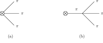
Figure 1: Diagrams contributing to the hadronic amplitude $T_{\pm\mu}$ at ${\cal O}(p^{2})$ $\chi$PT.

We now include the resonance–mediated contributions to the amplitude, to be evaluated through the interacting terms in ${\cal L}_{\rm R\chi T}$ Eq. (1). The relevant diagrams to be taken into account are those shown in Fig. 2. We get

$$T_{\pm\mu}^{R} = \mp\frac{\sqrt{2}\,F_{V}\,G_{V}}{3\,F^{3}}\;\left[\alpha(Q^{2},s,t)\,V_{1\mu}+\alpha(Q^{2},t,s)\,V_{2\mu}\right]$$ (10)

$$\pm\frac{4\,F_{A}\,G_{V}}{3\,F^{3}}\,\frac{Q^{2}}{Q^{2}-M_{A}^{2}}\,\left[\beta(Q^{2},s,t)\,V_{1\mu}+\beta(Q^{2},t,s)\,V_{2\mu}\right]\;.$$

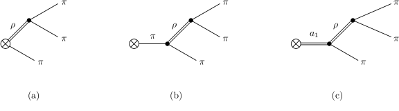
Figure 2: Resonance–mediated diagrams contributing to $T_{\pm\mu}$.

The functions $\alpha(Q^{2},s,t)$ and $\beta(Q^{2},s,t)$ are :

$$\alpha(Q^{2},s,t)\,=\,-\,3\,\frac{s}{s-M_{V}^{2}}\,+\,\left(\frac{2G_{V}}{F_{V}}-1\right)\,\left\{\,\frac{2Q^{2}-2s-u}{s-M_{V}^{2}}\,+\,\frac{u-s}{t-M_{V}^{2}}\,\right\}\;\;,$$ (11)

$$\beta(Q^{2},s,t)\,=\,-\,3\,(\lambda^{\prime}+\lambda^{\prime\prime})\,\frac{s}{s-M_{V}^{2}}\,+\,\,F(Q^{2},s)\,\frac{2Q^{2}+s-u}{s-M_{V}^{2}}\,+\,F(Q^{2},t)\,\frac{u-s}{t-M_{V}^{2}}\,\;\;,$$ (12)

with

$$F(Q^{2},s)=-\,\lambda_{0}\,\frac{m_{\pi}^{2}}{Q^{2}}\,+\,\lambda^{\prime}\,\frac{s}{Q^{2}}\,+\,\lambda^{\prime\prime}\;,$$ (13)

and depend on three combinations of the $\lambda_{i}$ couplings in ${\cal L}_{\rm R\chi T}$, that we call $\lambda_{0}$, $\lambda^{\prime}$ and $\lambda^{\prime\prime}$. Following the ideas outlined above we can get information on these combinations by implementing known aspects of asymptotic QCD. In particular we expect that the form factor of the axial-vector current into three pions should vanish at infinite transfer of momentum ($Q^{2}\rightarrow\infty$). This is a consequence of the fact that its contribution to the spectral function of the axial-vector current correlator, being positive, has to add to other infinite hadronic positive contributions to reach the constant value evaluated within QCD Floratos:1978jb . Accordingly the proper behaviour of the $T_{\pm\mu}$ form factor imposes the constraints :

$$2\,\lambda^{\prime}\,-\,1 = 0\;\;,$$

$$\lambda^{\prime\prime} = 0\;\;.$$ (14)

Hence there is only one combination of couplings left unknown, namely $\lambda_{0}$.

Finally an additional comment on the result for $T_{\pm\mu}^{R}$ is required. The form factors in Eq. (10) include zero–width $\rho$(770) and $a_{1}$(1260) propagator poles, leading to divergent phase–space integrals in the calculation of the $\tau\to\pi\pi\pi\nu_{\tau}$ decay width as the kinematical variables go along the full energy spectrum. The result can be regularized through the inclusion of resonance widths, which means to go beyond the leading order in the $1/N_{C}$ expansion, and implies the introduction of some additional theoretical inputs. This issue has been analysed in detail within the resonance chiral effective theory in Ref. GomezDumm:2000fz and, accordingly, we include off–shell widths for both resonances GomezDumm:2003ku .

4 Theory versus Experiment

To analyse the experimental data we will only consider the dominating $J^{P}=1^{+}$ driven axial–vector form factors, that satisfy $T_{+\mu}=-T_{-\mu}$ hence providing the same predictions for both $\tau^{-}\to\pi^{+}\pi^{-}\pi^{-}\nu_{\tau}$ and $\tau^{-}\to\pi^{-}\pi^{0}\pi^{0}\nu_{\tau}$ processes in the isospin limit.

We have fitted the experimental values for the $\tau^{-}\to\pi^{+}\pi^{-}\pi^{-}\nu_{\tau}$ branching ratio and normalized spectral function obtained by ALEPH Barate:1998uf and we get a reasonable $\chi^{2}/d.o.f.=64.5/52$. This is shown in Fig. 3.

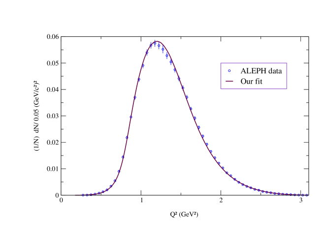
Figure 3: Fit to the ALEPH data Barate:1998uf for the normalized $\tau^{-}\rightarrow\pi^{+}\pi^{-}\pi^{-}\nu_{\tau}$.

Hence we get the axial–vector $a_{1}(1260)$ parameters $M_{A}=(1.203\pm 0.003)\,\mbox{GeV}$ and $\Gamma_{a_{1}}(M_{A}^{2})=(0.48\pm 0.02)\,\mbox{GeV}$, where the errors are only statistical. We also obtain a value for the still unknown combination of $\lambda_{i}$ couplings : $\lambda_{0}=11.9\pm 0.4$. However, as pointed out in Ref. Cirigliano:2004ue , this value seems too large when additional QCD constraints are imposed. The origin of the discrepancy could be the small sensitivity of the tau decay amplitude to this parameter, as it only appears multiplied by the mass of the pion (13), together with an improvable implementation of the off-shell width of the $a_{1}(1260)$ resonance.

Ultimately we predict the integrated structure functions $w_{A}$, $w_{C}$, $w_{D}$ and $w_{E}$ Kuhn:1992nz , that we compare with the experimental results for $\tau^{-}\to\pi^{-}\pi^{0}\pi^{0}\nu_{\tau}$ in Fig. 4. In spite of the large errors the predictions follow notably the depicted trend. As analysed in Ref. GomezDumm:2003ku a variance between the ALEPH data on one side and the OPAL and CLEO-II on the other are at the origin of the seemingly inconsistent result for $w_{A}$ in the high $Q^{2}$ region.

In conclusion it can be inferred that, within the present experimental errors and for the studied observables, there is no evidence of relevant contributions in $\tau\to\pi\pi\pi\nu_{\tau}$ decays beyond those of the $\rho(770)$ and $a_{1}(1260)$ resonances.

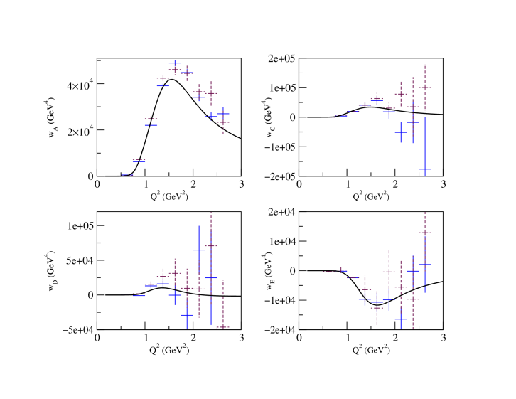
Figure 4: Theoretical values for the $w_{A}$, $w_{C}$, $w_{D}$ and $w_{E}$ integrated structure functions in comparison with the experimental data from CLEO-II (solid) and OPAL (dashed) Ackerstaff:1997dv .

References

• (1) A. Pich, “QCD Tests From Tau Decay Data,” Talk given at Tau Charm Factory Workshop, Stanford, Calif., May 23-27, 1989 ; J. H. Kuhn and A. Santamaria, Z. Phys. C 48 (1990) 445.
• (2) N. N. Achasov and A. A. Kozhevnikov, Phys. Rev. D 55 (1997) 2663 [arXiv:hep-ph/9609216].
• (3) J. Portolés, Nucl. Phys. Proc. Suppl.  98 (2001) 210 [arXiv:hep-ph/0011303];
• (4) D. Gómez Dumm, A. Pich and J. Portolés, Phys. Rev. D 69 (2004) 073002 [arXiv:hep-ph/0312183].
• (5) J. Portolés, Nucl. Phys. Proc. Suppl.  144 (2005) 3 [arXiv:hep-ph/0411333].
• (6) S. Weinberg, PhysicaA 96 (1979) 327; J. Gasser and H. Leutwyler, Annals Phys.  158 (1984) 142.
• (7) G. Colangelo, M. Finkemeier and R. Urech, Phys. Rev. D 54 (1996) 4403 [arXiv:hep-ph/9604279].
• (8) R. Barate et al. [ALEPH Collaboration], Eur. Phys. J. C 4 (1998) 409.
• (9) K. Ackerstaff et al. [OPAL Collaboration], Z. Phys. C 75 (1997) 593; T. E. Browder et al. [CLEO Collaboration], Phys. Rev. D 61 (2000) 052004 [arXiv:hep-ex/9908030].
• (10) G. Ecker, J. Gasser, A. Pich and E. de Rafael, Nucl. Phys. B 321 (1989) 311.
• (11) G. Ecker, J. Gasser, H. Leutwyler, A. Pich and E. de Rafael, Phys. Lett. B 223 (1989) 425.
• (12) G. ’t Hooft, Nucl. Phys. B 75 (1974) 461; E. Witten, Nucl. Phys. B 160 (1979) 57.
• (13) A. Pich, in Proceedings of the Phenomenology of Large $N_{C}$ QCD, edited by R. Lebed (World Scientific, Singapore, 2002), p. 239, arXiv:hep-ph/0205030.
• (14) J. H. Kuhn and E. Mirkes, Z. Phys. C 56 (1992) 661 [Erratum-ibid. C 67 (1995) 364].
• (15) D. Gomez Dumm, A. Pich and J. Portolés, Phys. Rev. D 62 (2000) 054014 [arXiv:hep-ph/0003320].
• (16) E. G. Floratos, S. Narison and E. de Rafael, Nucl. Phys. B 155 (1979) 115.
• (17) V. Cirigliano, G. Ecker, M. Eidemuller, A. Pich and J. Portolés, Phys. Lett. B 596 (2004) 96 [arXiv:hep-ph/0404004].