Detecting solar axions using Earth’s magnetic field

Abstract

We show that solar axion conversion to photons in the Earth’s magnetosphere can produce an x-ray flux, with average energy $\langle{\omega}\rangle\simeq 4\,\mathrm{keV}$, which is measurable on the dark side of the Earth. The smallness of the Earth’s magnetic field is compensated by a large magnetized volume. For axion masses $m_{a}\lesssim 10^{-4}\,\mathrm{eV}$, a low-Earth-orbit x-ray detector with an effective area of $10^{4}\,\mathrm{cm}^{2}$, pointed at the solar core, can probe the photon-axion coupling down to $10^{-11}\,\mathrm{GeV}^{-1}$, in one year. Thus, the sensitivity of this new approach will be an order of magnitude beyond current laboratory limits.

The existence of weakly interacting light pseudo-scalars is well-motivated in particle physics. For example, experimental evidence requires the size of $CP$ violation in strong interactions, as parameterized by the angle $\theta$, to be very tiny; $\theta\lesssim 10^{-10}$. However, there is no symmetry reason within the Standard Model (SM) for such a small $\theta$ angle; this is the strong $CP$ problem. An elegant solution to this puzzle was proposed by Peccei and Quinn Peccei:1977hh , where a new $U(1)$ symmetry, anomalous under strong interactions, was proposed. This $U(1)$ symmetry is assumed to be spontaneously broken at a scale $f_{a}$, resulting in a pseudo-scalar Goldstone boson $a$ Weinberg:1977ma , the axion. Non-perturbative QCD interactions at the scale $\Lambda_{\rm QCD}\sim 100\,\mathrm{MeV}$ generate a potential for the axion, endowing it with a mass $m_{a}\sim\Lambda_{\rm QCD}^{2}/f_{a}$. Experimental and observational bounds have pushed $f_{a}$ to scales of order $10^{7}\,\mathrm{GeV}$, which sets the inverse coupling of the axion to the SM fields. Thus the current data suggests that the axion is basically ‘invisible’ and very light, with $m_{a}\lesssim 1\,\mathrm{eV}$. Apart from the above considerations, axion-type particles are also ubiquitous in string theory.

The coupling of the axion to photons is given by

$${\cal L}_{a\gamma}=-\frac{a}{4M}F_{\mu\nu}{\tilde{F}}^{\mu\nu},$$ (1)

where $M\sim(\pi/\alpha)f_{a}$, $\alpha\simeq 1/137$ is the fine structure constant, and $F_{\mu\nu}$ is the electromagnetic field strength. The interaction in (1) makes it possible for hot plasmas, like the Sun, to emit a flux of axions through the Primakoff process Primakoff . This same interaction has also led to experimental proposals Sikivie:1983ip for detecting the axion through its conversion to photons in external magnetic fields. Various experimental bounds, most recent of which is set by the CAST experiment Andriamonje:2004hi , suggest that $g_{a\gamma}\equiv M^{-1}\lesssim 10^{-10}\,\mathrm{GeV}^{-1}$, as shown in Fig. (1). Here we note that some cosmological considerations related to overclosure of the universe suggest a lower bound $g_{a\gamma}\gtrsim 10^{-15}\,\mathrm{GeV}^{-1}$ Preskill:1982cy . For a review of different bounds on axion couplings, see Ref. Eidelman:2004wy .

In what follows, we propose a new approach for detecting solar axions, via their conversion to an x-ray flux in the magnetosphere near a planet, using a detector in orbit . The possibility of using planetary magnetic fields as a conversion region for high energy cosmic axions was discussed in Ref. Zioutas:1998ra . We take Earth as our reference example and consider the upward flux of axions going through the Earth and exiting on the night side . This setup provides an effective way of removing the solar x-ray background. The radius of the Earth is $R_{\oplus}\approx 6.4\times 10^{3}\,\mathrm{km}$ and its magnetic field is well approximated by a dipole for distances less than $1000\,\mathrm{km}$ above the surface. The field strength is $B_{\oplus}\simeq 3\times 10^{-5}\,\mathrm{T}$ at the equator and it drops as $1/r^{3}$ Landolt . However, over distances $L\ll R_{\oplus}$, we may assume $B_{\oplus}=const$. We will later show that we are interested in $L<1000\,\mathrm{km}$, for which this is a valid assumption.

The Earth’s atmosphere is mostly composed of nitrogen and oxygen. Solar axions have an average energy $\langle{\omega_{a}}\rangle\simeq 4\,\mathrm{keV}$ vanBibber:1988ge , which upon conversion in the magnetosphere will turn into x-ray photons of the same energy. The absorption length $\lambda_{\rm x}$ for 4-keV x-rays in the Earth’s atmosphere is about $10\,\mathrm{cm}$ at sea-level X-ray . However, at an altitude of $150\,\mathrm{km}$, atmospheric pressure falls to about $10^{-10}\,\mathrm{atm}$. For an ideal gas, density is proportional to pressure. Since the absorption length of a photon is inversely proportional to the density of scatterers, it follows that the x-ray absorption length scales as the inverse of pressure. Thus, above an altitude of $150\,\mathrm{km}$, $\lambda_{\rm x}\sim 10^{6}\,{\rm km}\sim(10^{-16}{\,\mathrm{eV}})^{-1}$ is a lower bound. Since we will mostly consider $L\gg 150\,\mathrm{km}$, this lower bound holds over distances of interest to us.

The axion to photon conversion probability, in a transverse magnetic field of strength $B$, is given by Raffelt:1987im ; vanBibber:1988ge

$$p_{\gamma}(L)=\left(\frac{B}{2M}\right)^{2}\left[\frac{1+e^{-\Gamma L}-2e^{-\Gamma L/2}\cos(qL)}{q^{2}+(\Gamma^{2}/4)}\right],$$ (2)

where $L$ is the path length traveled by the axion, $\Gamma=\lambda_{\rm x}^{-1}$ is set by the absorption length, and $\ell=2\pi/q$ is the oscillation length. Here, we have

$$q=\left|m_{\gamma}^{2}-m_{a}^{2}\right|/(2\omega_{a}),$$ (3)

with $m_{\gamma}$ the plasma mass of the photon. Since the atmospheric pressure drops to below $10^{-10}\,\mathrm{atm}$ at altitudes small compared to $L\sim 1000\,\mathrm{km}$, it is safe to ignore $m_{\gamma}$. To see this, first note that the largest electron binding energies for nitrogen and oxygen are well below $1\,\mathrm{keV}$ X-ray , therefore the energy dependence of $m_{\gamma}^{2}$ is not complicated by resonant scattering for x-rays of energy near $4\,\mathrm{keV}$. Thus, $m_{\gamma}^{2}$ is proportional to the density and hence to the pressure of the gas. At $1\,\mathrm{atm}$, the plasma mass of 4-keV x-rays is $m_{\gamma}\sim 1\,\mathrm{eV}$. This suggests that above an altitude of $150\,\mathrm{km}$, where the pressure falls below $10^{-10}\,\mathrm{atm}$, $m_{\gamma}$ is less than $\sim 10^{-5}\,\mathrm{eV}$, and hence below the range we consider for $m_{a}$, as seen from Fig. 1. Given an oscillation length $L\sim 1000\,\mathrm{km}$, we are sensitive to $m_{a}\sim 10^{-4}\,\mathrm{eV}$. For this value of $m_{a}$, we get $q\sim 10^{-12}\,\mathrm{eV}\gg\Gamma$, where $\Gamma=\lambda_{\rm x}^{-1}\lesssim 10^{-16}\,\mathrm{eV}$; we may safely ignore $\Gamma$ in our treatment.

Hence, we can write Eq.(2) as

$$p_{\gamma}(L)=2\left(\frac{B}{2M}\right)^{2}\left[\frac{1-\cos(qL)}{q^{2}}\right],$$ (4)

For $m_{a}\leq 10^{-4}\,\mathrm{eV}$, $M=10^{10}\,\mathrm{GeV}$, $B=B_{\oplus}=3\times 10^{-5}\,\mathrm{T}$, $\omega=4\,\mathrm{keV}$, and $L=L_{\oplus}=\pi/q_{\rm max}\simeq 600\,\mathrm{km}$, we then find $p_{\gamma}(L_{\oplus})\approx 10^{-18}$. Here, $q_{\rm max}$ corresponds to $m_{a}=10^{-4}\,\mathrm{eV}$. Given that the flux of solar axions at Earth is vanBibber:1988ge ; Andriamonje:2004hi

$$\Phi_{a}=3.67\times 10^{11}(10^{10}\,{\rm GeV}/M)^{2}\,{\rm axions}\,{\rm cm}^{-2}\,{\rm s}^{-1},$$ (5)

the expected flux of x-rays at an altitude of about $L_{\oplus}$ near the equator, for $M=10^{10}\,\mathrm{GeV}$, is

$$\Phi_{\gamma}(L_{\oplus})\approx 4\times 10^{-7}\,{\rm photons}\,{\rm cm}^{-2}\,{\rm s}^{-1}.$$ (6)

Then, for an effective detector area $A\sim 10^{4}\,\mathrm{cm}^{2}$ and running time $\delta t\sim 10^{7}\,\mathrm{s}$, the number of x-ray photons observed is $N_{\gamma}\sim 10^{4}$. The signal decreases as $g_{a\gamma}^{4}$, and thus this number of events can constrain $g_{a\gamma}$ to near $10^{-11}\,\mathrm{GeV}^{-1}$. Hence, in the regime $m_{a}\lesssim 10^{-4}\,\mathrm{eV}$, the low-Earth orbit observations can be sensitive to couplings roughly one order of magnitude smaller than the current laboratory limits. Figure 1 shows the expected x-ray flux at $L_{\oplus}=600\,\mathrm{km}$ as a function of $m_{a}$ and $g_{a\gamma}$. For this plot we integrated the conversion probability as given in Eq. (4) folded with solar axion spectrum vanBibber:1988ge ; Andriamonje:2004hi over axion energies from $1-10\,\mathrm{keV}$.

Here, we would like to note that matching $m_{a}$ and $m_{\gamma}$ results in resonant axion-photon conversion, which in principle can enhance the signal for $m_{a}\neq 0$ vanBibber:1988ge ; Raffelt:1987im . For the solar axions we consider, there could be a similar effect in the Earth’s atmosphere. However, it turns out that the thickness of any such resonant layer is always small compared to the oscillation length of axions and therefore no enhancement results.

It is instructive to have a simple quantitative comparison between our space-based method and that of laboratory experiments like CAST. Here, we will estimate the figure of merit ${\cal F}$ for each approach. We note that in the low mass region of interest to us, the conversion probability scales as $(BL)^{2}$. Therefore, we define ${\cal F}\equiv BL$. For the CAST experiment, the transverse magnetic field $B\approx 10\,\mathrm{T}$ and the length of the magnetized region $L\approx 10\,\mathrm{m}$ Andriamonje:2004hi . Thus, ${\cal F}({\rm CAST})\approx 100\,\mathrm{T}\,\mathrm{m}$. For the technique presented in this paper, we have $B_{\oplus}\approx 3\times 10^{-5}\,\mathrm{T}$ and $L_{\oplus}\approx 600\,\mathrm{km}$, hence ${\cal F}_{\oplus}\approx 18\,\mathrm{T}\,\mathrm{m}$. We see that our approach has a figure of merit 5 times smaller than that of the CAST experiment. However, the effective magnetized cross-sectional area of the CAST experiment is about $14\,\mathrm{cm}^{2}$ Andriamonje:2004hi . In our case, since the magnetized region has a size of order $1000\,\mathrm{km}$, the cross sectional area is only limited by the detector size, which is of order $10^{4}\,\mathrm{cm}^{2}$. Hence, given the same length of time, the space-based technique detailed above has higher sensitivity than the CAST experiment, for $m_{a}\lesssim 10^{-4}\,\mathrm{eV}$.

The above exposition assumes that there are no backgrounds to the measurement, which in any realistic experiment is not the case. Since it is difficult to reliably estimate the background from first principles, it is useful to look at actual x-ray experiments.

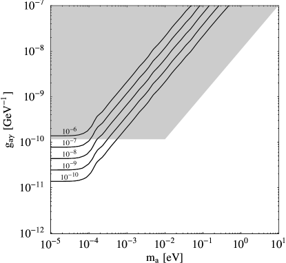
Figure 1: X-ray flux from axion conversion in units of $\mathrm{photons}\,\mathrm{cm}^{-2}\,\mathrm{s}^{-1}$ in the range from $1-10\,\mathrm{keV}$ for an orbit of $600\,\mathrm{km}$. The uppermost line corresponds to the sensitivity of existing satellites, whereas the lowermost line could be obtained by future missions. The shaded area schematically depicts the CAST $95\%$ C.L. excluded region Andriamonje:2004hi .

One example is the ‘Rossi x-ray timing explorer’ (RXTE) launched in the mid 90’s rxte . It has an effective x-ray collection area of $\sim 7\,000\,\mathrm{cm}^{2}$ and is sensitive over $1-50\,\mathrm{keV}$. Its angular resolution is roughly $0.5^{\circ}$. It orbits the Earth at a height of $\sim 600\,\mathrm{km}$. During slews and calibration from 1996 till 1999 it has acquired at least $25\,000\,\mathrm{s}$ of viewing the night side of the Earth. The nominal background when watching the blank sky is about 3 counts per second in the energy range from $2-10\,\mathrm{keV}$ over the whole effective area Revnivtsev:2003wm . Thus there are $7.5\times 10^{4}$ background events in $25\,000\,\mathrm{s}$, whose fluctuations are given by $\sqrt{7.5\times 10^{4}}\sim 270$; dividing this by the exposure and area gives a sensitivity of $1.5\times 10^{-6}\,\mathrm{photons}\,\mathrm{cm}^{-2}\,\mathrm{s}^{-1}$. Although this experiment was not designed to perform our type of observation, this level of sensitivity would allow to probe axion couplings $g_{a\gamma}$ of the order $10^{-10}\,\mathrm{GeV}^{-1}$, which is shown in Fig. 1.

Another example is the LOBSTER lobster experiment planned to fly on the International Space Station, which has an orbit of $350\,\mathrm{km}$. It will have a total x-ray collection area of $\sim 10^{4}\,\mathrm{cm}^{2}$, its angular resolution is approximately $3^{\prime}$ and it is sensitive from $0.5-3.5\,\mathrm{keV}$. It has a background rate per pixel (the solar core where axions are produced covers approximately 1 pixel) of $10^{-5}\,\mathrm{s}^{-1}$. Thus, in $10^{7}\,\mathrm{s}$ of observation they have $100$ background events and the background fluctuation is $\sqrt{100}=10$ events. Therefore, we have a sensitivity of $10/10^{4}/10^{7}=10^{-10}\,\mathrm{photons}\,\mathrm{cm}^{-2}\,\mathrm{s}^{-1}$, which in turn, according to Fig. 1, gives a limit on $g_{a\gamma}$ of order $10^{-11}\,\mathrm{GeV}^{-1}$.

Given the above considerations, existing or planned orbital x-ray telescopes can be used for solar axion detection, using the method proposed here. Therefore, a specialized and dedicated mission is not required to implement our approach. In fact, some of the existing x-ray data may already contain the information required for competitive or even better sensitivities than those obtained from current laboratory experiments. This depends on how much of the present x-ray calibration data has been obtained while the telescope was pointed at the core of the Sun, on the dark side of the Earth.

To summarize, in this Letter, we have proposed a new technique for detecting solar axions, using Earth’s magnetosphere. We have shown that given the large magnetized volume around the Earth, conversion of axions, with mass $m_{a}\lesssim 10^{-4}\,\mathrm{eV}$, into x-rays of average energy $\langle{\omega}\rangle\simeq 4\,\mathrm{keV}$ will be measurable by an x-ray telescope, in a low-Earth orbit. A key ingredient of our proposal is to use the Earth as an x-ray shield and look for axions coming through the Earth on the night side. This effectively removes the solar x-ray background. Thus, observation of x-rays, with a thermal energy distribution peaked at approximately $4\,\mathrm{keV}$, on the night side of the Earth is a distinct signature of solar axions in our proposal. Moreover these x-rays would only come from the center of the Sun, which subtends approximately $3^{\prime}$ and there would be an orbital variation with magnetic field strength and an annual modulation by the Sun-Earth distance. Considering the well-established framework of the solar model, it would be extremely difficult to come up with an alternative explanation of all these signatures. Therefore, our method can achieve an unambiguous detection of solar axions. We estimate that, in a one-year run, this technique will gain sensitivity to axion-photon couplings of order $g_{a\gamma}\sim 10^{-11}\,\mathrm{GeV}^{-1}$, about an order of magnitude beyond current laboratory limits. We conclude that, for solar axions in the regime considered here, our approach will probe axion-photon couplings beyond the reach of foreseeable laboratory experiments.

- (1) R. D. Peccei and H. R. Quinn, Phys. Rev. Lett. 38, 1440 (1977); Phys. Rev. D 16, 1791 (1977).
- (2) S. Weinberg, Phys. Rev. Lett. 40, 223 (1978); F. Wilczek, ibid. 40, 279 (1978).
- (3) H. Primakoff, Phys. Rev. 81, 899 (1951).
- (4) P. Sikivie, Phys. Rev. Lett. 51, 1415 (1983) [Erratum-ibid. 52, 695 (1984)].
- (5) K. Zioutas et al. [CAST Collaboration], Phys. Rev. Lett. 94, 121301 (2005) [arXiv:hep-ex/0411033].
- (6) J. Preskill, M. B. Wise and F. Wilczek, Phys. Lett. B 120, 127 (1983); L. F. Abbott and P. Sikivie, Phys. Lett. B 120, 133 (1983); M. Dine and W. Fischler, Phys. Lett. B 120, 137 (1983); M. S. Turner, Phys. Rev. D 33, 889 (1986).
- (7) S. Eidelman et al. [Particle Data Group], Phys. Lett. B 592, 1 (2004).
- (8) K. Zioutas, D. J. Thompson and E. A. Paschos, Phys. Lett. B 443, 201 (1998) [arXiv:astro-ph/9808113].
- (9) Landolt-Börnstein, New Series, Volume 2b, Geophysics of the Solid Earth, the Moon and the Planets, pp 31-99, Springer, Berlin, 1985.
- (10) K. van Bibber, P. M. McIntyre, D. E. Morris and G. G. Raffelt, Phys. Rev. D 39, 2089 (1989).
- (11) Ed. Emmett F. Kaelble, Handbook of X-rays, McGraw Hill, New York, 1967.
- (12) G. Raffelt and L. Stodolsky, Phys. Rev. D 37, 1237 (1988).
- (13) K Jahoda et al, Proc. SPIE Vol. 2808, p. 59-70, EUV, X-Ray, and Gamma-Ray Instrumentation for Astronomy VII, Oswald H. Siegmund; Mark A. Gummin; Eds.
- (14) M. Revnivtsev, M. Gilfanov, R. Sunyaev, K. Jahoda and C. Markwardt, Astron. Astrophys. 411, 329 (2003) [arXiv:astro-ph/0306569].
- (15) W. C. Priedhorsky, A. G. Peele and K. A. Nugent, Mon. Not. R. Astronom. Soc. 279, 733-750, (1996)