Random Matrices

Abstract

We review elementary properties of random matrices and discuss widely used mathematical methods for both hermitian and nonhermitian random matrix ensembles. Applications to a wide range of physics problems are summarized. This paper originally appeared as an article in the Wiley Encyclopedia of Electrical and Electronics Engineering.

Introduction

In general, random matrices are matrices whose matrix elements are stochastic variables. The main goal of Random Matrix Theory (RMT) is to calculate the statistical properties of eigenvalues for very large matrices which are important in many applications. Ensembles of random matrices first entered in the mathematics literature as a $p$-dimensional generalization of the $\chi^{2}$-distribution Wishart . Ensembles of real symmetric random matrices with independently distributed Gaussian matrix elements were introduced in the physics literature in order to describe the spacing distribution of nuclear levels Wigner . The theory of Hermitian random matrices was first worked out in a series of seminal papers by Dyson Dyson . Since then, RMT has had applications in many different branches of physics ranging from sound waves in aluminum blocks to quantum gravity. For an overview of the early history of RMT we refer to the book by Porter Porter . An authoritative source on RMT is the book by Mehta Meht91 . For a comprehensive review including the most recent developments we refer to Ref. Guhr98 .

Generally speaking, random matrix ensembles provide a statistical description of a complex interacting system. Depending on the hermiticity properties of the interactions, one can distinguish two essentially different classes of random matrices: Hermitian matrices with real eigenvalues and matrices without hermiticity properties with eigenvalues scattered in the complex plane. We will first give an overview of the ten different classes of Hermitian random matrices and then briefly discuss non-Hermitian random matrix ensembles.

The best known random matrix ensembles are the Wigner-Dyson ensembles which are ensembles of Hermitian matrices with matrix elements distributed according to

$$P(H)DH={\cal N}e^{-\frac{N\beta}{4}{\rm Tr}H^{\dagger}H}DH.$$ (1)

Here, $H$ is a Hermitian $N\times N$ matrix with real, complex, or quaternion real matrix elements. The corresponding random matrix ensemble is characterized by the Dyson index $\beta=1,$ 2, and 4, respectively. The measure $DH$ is the Haar measure which is given by the product over the independent differentials. The normalization constant of the probability distribution is denoted by ${\cal N}$. The probability distribution (1) is invariant under the transformation

$$H\rightarrow UHU^{-1},$$ (2)

where $U$ is an orthogonal matrix for $\beta=1$, a unitary matrix for $\beta=2$, and a symplectic matrix for $\beta=4$. This is the reason why these ensembles are known as the Gaussian Orthogonal Ensemble (GOE), the Gaussian Unitary Ensemble (GUE), and the Gaussian Symplectic Ensemble (GSE), respectively. The GOE is also known as the Wishart distribution. Since both the eigenvalues of $H$ and the Haar measure $DH$ are invariant with respect to (2), the eigenvectors and the eigenvalues are independent with the distribution of the eigenvectors given by the the invariant measure of the corresponding orthogonal, unitary, or symplectic group.

There are two ways of arriving at the probability distribution (1). First, from the requirement that the matrix elements are independent and are distributed with the same average and variance for an ensemble invariant under (2). Second, by requiring that the probability distribution maximizes the information entropy subject to the constraint that the average and the variance of the matrix elements are fixed.

A second class of random matrices are the chiral ensembles Verb94a with the chiral symmetries of the QCD Dirac operator. They are defined as the ensembles of $N\times N$ Hermitian matrices with block structure

$$H=\left(\begin{array}[]{cc}0&C\\ C^{\dagger}&0\end{array}\right)$$ (5)

and probability distribution given by

$$P(C)DC={\cal N}{\det}^{N_{f}}\left(\begin{array}[]{cc}0&C\\ C^{\dagger}&0\end{array}\right)e^{-\frac{N\beta}{4}{\rm Tr}C^{\dagger}C}DC.$$ (8)

Again, $DC$ is the Haar measure, and $N_{f}$ is a real parameter (corresponding to the number of quark flavors in QCD). The matrix $C$ is a rectangular $n\times(n+\nu)$ matrix. Generically, the matrix $H$ in (5) has exactly $|\nu|$ zero eigenvalues. Also generically, the QCD Dirac operator corresponding to a field configuration with the topological charge $\nu$ has exactly $|\nu|$ zero eigenvalues, in accordance with the Atiyah-Singer index theorem. For this reason, $\nu$ is identified as the topological quantum number. The normalization constant of the probability distribution is denoted by ${\cal N}$. Also in this case one can distinguish ensembles with real, complex, or quaternion real matrix elements. They are denoted by $\beta=1$, $\beta=2$, and $\beta=4$, respectively. The invariance property of the chiral ensembles is given by

$$C\rightarrow UCV^{-1},$$ (9)

where $U$ and $V$ are orthogonal, unitary, and symplectic matrices, respectively. For this reason, the corresponding ensembles are known as the chiral Gaussian Orthogonal Ensemble (chGOE), the chiral Gaussian Unitary Ensemble (chGUE), and the chiral Gaussian Symplectic Ensemble (chGSE), respectively. A two sub-lattice model with diagonal disorder in the chGUE class was first considered in Gade .

A third class of random matrix ensembles occurs in the description of disordered superconductors. Such ensembles with the symmetries of the Bogoliubov-de Gennes Hamiltonian have the block structure

$$H=\left(\begin{array}[]{cc}A&B\\ B^{\dagger}&-A^{T}\end{array}\right),$$ (12)

where $A$ is Hermitian and, depending on the underlying symmetries, the matrix $B$ is symmetric or anti-symmetric. The probability distribution is given by

$$P(H)DH={\cal N}\exp\left(-\frac{N\beta}{4}{\rm Tr}H^{\dagger}H\right)DH,$$ (13)

where $DH$ is the Haar measure and ${\cal N}$ is a normalization constant. For symmetric $B$ the matrix elements of $H$ can be either complex (C) or real (CI). For anti-symmetric $B$ the matrix elements of $H$ can be either complex (D) or quaternion real (DIII). The name of the ensembles (in parentheses) refers to the symmetric space to which they are tangent to. Since they were first introduced by Altland and Zirnbauer AZ ; class we will call them the Altland-Zirnbauer ensembles. A hopping model based on the class CI first entered in Oppermann .

A key ingredient in the classification of a Hamiltonian in terms of one of the above random matrix ensembles is its anti-unitary symmetries. An anti-unitary operator can be written as

$$U=AK,$$ (14)

where $A$ is unitary and $K$ is the complex conjugation operator. For the classification according to the anti-unitary symmetries we can restrict ourselves to the following three different possibilities: (i) the Hamiltonian does not have any anti-unitary symmetries, (ii) the Hamiltonian commutes with $AK$ and $(AK)^{2}=1$, and (iii) $[H,AK]=0$ but $(AK)^{2}=-1$. In the first case, the matrix elements of the Hamiltonian are complex, in the second case, it is always possible to find a basis in which the Hamiltonian is real, and in the third case, it can be shown that it is possible to organize the matrix elements of the Hamiltonian in quaternion real elements. These three different possibilities are denoted by the number of degrees of freedom per matrix element, $\beta=2$, $\beta=1$, and $\beta=4$, respectively. This triality characterizes the Wigner-Dyson ensembles, the chiral ensembles, and the Altland-Zirnbauer ensembles. In most cases, the anti-unitary operator is the time-reversal symmetry operator. For systems without spin, this is just the complex conjugation operator. For systems with spin, the time reversal operator can be represented as $i\sigma_{2}K$, where $\sigma_{2}$ is one of the Pauli matrices.

RMT	symmetric space	$\beta$	$\alpha$
GOE	AI	1	—
GUE	A	2	—
GSE	AII	4	—
chGOE	BDI	1	$|\nu|+2N_{f}$
chGUE	AIII	2	$1+2|\nu|+2N_{f}$
chGSE	CII	4	$3+4|\nu|+2N_{f}$
AZ-CI	CI	1	1
AZ-D	D	2	0
AZ-C	C	2	2
AZ-DIII	DIII	4	1

Table 1: Random matrix ensemble, corresponding symmetric space, and the values for $\alpha$ and $\beta$.

We have introduced ten different random matrix ensembles. Each of these ensembles can be identified as the tangent space of one of the large families of symmetric spaces as classified by Cartan (see Table 1). The matrices in each of these ten ensembles can be diagonalized by a unitary transformation, with the unitary matrix distributed according to the group measure. For all ensembles, the Jacobian for the transformation to eigenvalues as new integration variables depends only on the eigenvalues. For an extensive discussion of the calculation of this type of Jacobian we refer to HUA . For the Wigner-Dyson ensembles, the joint probability distribution of the eigenvalues is given by

$$P(\{\lambda\})d\{\lambda\}={\cal N}|\Delta(\{\lambda\})|^{\beta}\prod_{k}e^{-N\beta\lambda_{k}^{2}/4}d\lambda_{k},$$ (15)

where the Vandermonde determinant is defined by

$$\Delta(\{\lambda\})=\prod_{k>l}(\lambda_{k}-\lambda_{l}).$$ (16)

This factor results in correlations of eigenvalues that are characteristic for the random matrix ensembles. For example, one finds repulsion of eigenvalues at small distances.

For the remaining ensembles, the eigenvalues occur in pairs $\pm\lambda_{k}$. This results in the distribution

$$P(\{\lambda\})d\{\lambda\}={\cal N}|\Delta(\{\lambda^{2}\})|^{\beta}\prod_{k}\lambda_{k}^{\alpha}e^{-N\beta\lambda_{k}^{2}/4}d\lambda_{k}.$$ (17)

The values of $\beta$ and $\alpha$ are given in Table 1 below.

Another well-known random matrix ensemble which is not in the above classification is the Poisson Ensemble defined as an ensemble of uncorrelated eigenvalues. Its properties are very different from the above RMTs where the diagonalization of the matrices leads to strong correlations between the eigenvalues.

The physical applications of RMT have naturally biased the interest of researchers to Hermitian matrices (e.g., the Hamiltonian of a quantum system is a Hermitian operator and should be represented by a Hermitian matrix). A variety of methods, described in this article, have been developed to treat ensembles of Hermitian matrices. In contrast, non-Hermitian random matrices received less attention. Apart from the intrinsic mathematical interest of such a problem, a number of physically important applications exist which warrant the study of non-Hermitian random matrices.

The simplest three classes of non-Hermitian random matrices, introduced by Ginibre Ginibre , are direct generalizations of the GOE, GUE, and GSE. They are given by an ensemble of matrices $C$ without any Hermiticity properties and a Gaussian probability distribution given by

$$P(C)DC={\cal N}e^{-\frac{N\beta}{2}{\rm Tr}C^{\dagger}C}DC\>,$$ (18)

where $DC$ is the product of the differentials of the real and imaginary parts of the matrix elements of $C$. Such matrices can be diagonalized by a similarity transformation with eigenvalues scattered in the complex plane. The probability distribution is not invariant under this transformation, and therefore the eigenvalues and the eigenvectors are not distributed independently. Similarly to the Hermitian ensembles, the matrix elements can be chosen real, arbitrary complex, or quaternion real.

The case of the arbitrary complex non-Hermitian random matrix ensemble (18) with $\beta=2$ is the simplest. The joint probability distribution of eigenvalues $\{\lambda\}=\{\lambda_{1},\ldots,\lambda_{N}\}$ is given by a formula similar to (15):

$$P(\{\lambda\})d\{\lambda\}={\cal N}|\Delta(\{\lambda\})|^{2}\prod_{k}e^{-N|\lambda_{k}|^{2}}dx_{k}dy_{k},$$ (19)

where $x_{k}={\rm Re\>}\lambda_{k}$, $y_{k}={\rm Im\>}\lambda_{k}$. In the quaternion-real case, the joint probability distribution can also be written explicitly. In the case of real matrices, the joint probability distribution is not known in closed analytical form.

It is also possible to introduce non-Hermitian ensembles with a chiral structure, but such ensembles have received very little attention in the literature and will not be discussed. What has received a great deal of attention in the literature are non-Hermitian deformations of the Hermitian random matrix ensembles. Among others, they enter in the statistical theory of $S$-matrix fluctuations VWZ , models of directed quantum chaos efetov ; fyodorov and in chiral random matrix models at nonzero chemical potential Step96 . The latter class of ensembles is obtained from (5) and (8) by making the replacement

$$\left(\begin{array}[]{cc}0&C\\ C^{\dagger}&0\end{array}\right)\rightarrow\left(\begin{array}[]{cc}0&C+i\mu\\ C^{\dagger}+i\mu&0\end{array}\right).$$ (24)

This chRMT is a model for the QCD partition function at nonzero chemical potential $\mu$ and will be discussed in more detail below.

Random Matrix Theory is a theory to describe the correlations of the eigenvalues of a differential operator. The correlation functions can be derived from the joint probability distribution. The simplest object is the spectral density

$$\rho(\lambda)=\sum_{k}\delta(\lambda-\lambda_{k}).$$ (25)

The average spectral density, denoted by

$$R_{1}(\lambda)=\langle\rho(\lambda)\rangle,$$ (26)

is obtained from the joint probability distribution by integration over all eigenvalues except one. The connected two-point correlation function is defined by

$$\rho_{c}(\lambda_{1},\lambda_{2})=\langle\rho(\lambda_{1})\rho(\lambda_{2})\rangle-\langle\rho(\lambda_{1})\rangle\langle\rho(\lambda_{2})\rangle.$$ (27)

In RMT it is customary to subtract the diagonal term from the correlation function and to introduce the two point correlation function $R_{2}(\lambda_{1},\lambda_{2})$ defined by

$$R_{2}(\lambda_{1},\lambda_{2})=\langle\rho(\lambda_{1})\rho(\lambda_{2})\rangle-\delta(\lambda_{1}-\lambda_{2})\langle\rho(\lambda)\rangle$$ (28)

and the two-point cluster function

$$T_{2}(\lambda_{1},\lambda_{2})=R_{1}(\lambda_{1})R_{1}(\lambda_{2})-R_{2}(\lambda_{1},\lambda_{2}).$$ (29)

In general, the $k-$point correlation function can be expressed in terms of the joint probability distribution $P_{N}$ as

$$R_{k}(\lambda_{1},...,\lambda_{k})=\frac{N!}{(N-k)!}\int_{-\infty}^{\infty}d\lambda_{k+1}\cdots d\lambda_{N}P_{N}(\lambda_{1},...,\lambda_{N}),$$ (30)

where we have included a combinatorial factor to account for the fact that spectral correlation functions do not distinguish the ordering of the eigenvalues. Similarly, one can define higher order connected correlation functions and cluster functions with all lower order correlations subtracted out. For details we refer to Mehta’s book Meht91 .

Instead of the spectral density one often studies the resolvent defined by

$$G(z)=\frac{1}{N}{\rm Tr}\frac{1}{z-H}=\frac{1}{N}\sum_{k=1}^{N}\frac{1}{z-\lambda_{k}}$$ (31)

which is related to the spectral density by

$$\langle\rho(\lambda)\rangle=-\lim_{\epsilon\rightarrow 0}\frac{N}{\pi}{\rm Im\>}\langle G(\lambda+i\epsilon)\rangle.$$ (32)

In the analysis of spectra of complex systems and the study of random matrix theories, it has been found that the average spectral density is generally not given by the result for the Gaussian random matrix ensembles which has a semi-circular shape. What is given by RMT are the correlations of the eigenvalues expressed in units of the average level spacing. For this reason one introduces the cluster function

$$Y_{2}(r_{1},r_{2})=\frac{T_{2}(r_{1}/R_{1}(\lambda_{1}),r_{2}/R_{1}(\lambda_{2}))}{R_{1}(\lambda_{1})R_{1}(\lambda_{2})}.$$ (33)

In general, correlations of eigenvalues in units of the average level spacing are called microscopic correlations. These are the correlations that can be described by the $N\rightarrow\infty$ limit of RMT.

The cluster function (33) has universal properties. In the limit $N\rightarrow\infty$, it is invariant with respect to modifications of the probability distribution of the random matrix ensemble. For example, for the GUE and the chGUE it has been shown that replacing the Gaussian probability distribution by a distribution given by the exponent of an arbitrary even polynomial results in the same microscopic correlation functions Hack ; Damgaard .

For ensembles in which the eigenvalues occur in pairs $\pm\lambda_{k}$, an additional important correlation function with universal properties is the microscopic spectral density Shur93 defined by

$$\rho_{s}(u)=\lim_{N\rightarrow\infty}\frac{1}{\pi\rho(0)}\left\langle\rho\left(\frac{u}{\pi\rho(0)}\right)\right\rangle.$$ (34)

Related to this observable is the distribution of the smallest eigenvalue which was shown to be universal as well Nish98 . For this class of ensembles, the point $\lambda=0$ is a special point. Therefore, all correlation functions near $\lambda=0$ have to be studied separately. However, the microscopic correlations of these ensembles in the bulk of the spectrum are the same as those of the Wigner-Dyson ensemble with the same value of $\beta$.

There are two different types of applications of RMT. First, as an exact theory of spectral correlations of a differential operator. As an important application we mention the study of universal properties in transport phenomena in nuclei VWZ and disordered mesoscopic systems. In particular, the latter topic has received a great deal of attention recently (see Guhr98 ; Beenreview ). This is the original application of RMT. Second, as a schematic model for a complex system. One famous example in the second class is the Anderson model Anderson for Anderson localization. The properties of this model depend in a critical way on the spatial dimensionality of the lattice. Other examples that will be discussed in more detail below are models for the QCD partition function at nonzero temperature and nonzero chemical potential.

Random Matrix Theory eigenvalue correlations are not found in all systems. Obviously, integrable systems, for example a harmonic oscillator, have very different spectral properties. Originally, in the application to nuclear levels, it was believed that the complexity of the system is the main ingredient for the validity of RMT. Much later it was realized that the condition for the presence of RMT correlations is that the corresponding classical system is completely chaotic. This so called Bohigas-Giannoni-Schmit conjecture Bohi84 was first shown convincingly for chaotic quantum billiards with two degrees of freedom. By now, this conjecture has been checked for many different systems, and with some well-understood exceptions, it has been found to be correct. However, a real proof is still absent, and it cannot be excluded that additional conditions may be required for its validity. In particular, the appearance of collective motion in complex many-body systems deserves more attention in this respect.

In general, the average spectral density is not given by RMT. Therefore, the standard procedure is to unfold the spectrum, i.e., to rescale the spacing between the eigenvalues according to the local average eigenvalue density. In practice, this unfolding procedure is done as follows. Given a sequence of eigenvalues $\{\lambda_{k}\}$ with average spectral density $\langle\rho(\lambda)\rangle$, the unfolded sequence is given by

$$\lambda_{k}^{u}=\int_{-\infty}^{\lambda_{k}}\langle\rho(\lambda)\rangle d\lambda.$$ (35)

The underlying assumption is that the average spectral density and the eigenvalue correlations factorize. The eigenvalue correlations of the unfolded eigenvalues can be investigated by means of suitable statistics. The best known statistics are the nearest neighbor spacing distribution $P(S)$, the number variance $\Sigma^{2}(r)$, and the $\Delta_{3}$ statistic. The number variance is defined as the variance of the number of eigenvalues in an interval of length $r$. The $\Delta_{3}$ statistic is related to the number variance by

$$\Delta_{3}(L)=\frac{2}{L^{4}}\int_{0}^{\infty}(L^{3}-2L^{2}r+r^{3})\Sigma^{2}(r)dr.$$ (36)

In the analysis of spectra it is essential to include only eigenstates with the same exact quantum numbers. Spectra with different exact quantum numbers are statistically independent.

The exact analytical expression of the RMT result for the nearest neighbor spacing distribution is rather complicated. However, it is well approximated by the Wigner surmise which is the spacing distribution for an ensemble of $2\times 2$ matrices. It is given by

$$P(S)=a_{\beta}S^{\beta}e^{-b_{\beta}S^{2}},$$ (37)

where the constants $a_{\beta}$ and $b_{\beta}$ can be fixed by the conditions that $P(S)$ is normalized to unity, and that the average level spacing is one. The level repulsion at short distances is characteristic for interacting systems. For uncorrelated eigenvalues one finds $P(S)=\exp(-S)$.

Another characteristic feature of RMT spectra is the spectral stiffness. This is expressed by the number variance which, asymptotically for large $r$, is given by

$$\Sigma^{2}(r)\sim\frac{2}{\beta\pi^{2}}\log r.$$ (38)

This should be contrasted with the result for uncorrelated eigenvalues given by $\Sigma^{2}(r)=r$.

In the analysis of spectra one often relies on spectral ergodicity defined as the equivalence of spectral averaging and ensemble averaging. This method cannot be used for the distribution of the smallest eigenvalues, and one necessarily has to rely on ensemble averaging.

Before proceeding to the discussion of mathematical methods of Random Matrix Theory a comment about the notations should be made. Different conventions for normalizing the variance of the probability distribution appear in the literature. This simply amounts to a rescaling of the eigenvalues. For example, in the discussion of orthogonal polynomials and the Selberg integral below, introduction of rescaled eigenvalues such as $\lambda_{k}\sqrt{N/2}$ or $\lambda_{k}\sqrt{N}$ simplifies the expressions.

Mathematical methods I: Hermitian Matrices

Orthogonal polynomials.

One of the oldest and perhaps most widely used methods in RMT is based on orthogonal polynomials. A comprehensive presentation of this method is given in Mehta’s book Meht91 . Here, we summarize the most important ingredients, concentrating on the GUE for mathematical simplicity.

We have seen in the introductory chapter that the spectral correlation functions can be obtained by integrating the joint probability distribution. The mathematical problem consists in performing these integrations in the limit $N\to\infty$. It is convenient to rescale $\lambda_{k}$ and introduce $x_{k}=\lambda_{k}\sqrt{N/2}$. The main point of the orthogonal-polynomial method is the observation that the Vandermonde determinant can be rewritten in terms of orthogonal polynomials $p_{n}(x)$ by adding to a given row appropriate linear combinations of other rows,

$$\Delta(\{x\})=\det\left[(x_{j})^{i-1}\right]_{ij}={\rm const}\times\det\left[p_{i-1}(x_{j})\right]_{ij}\>.$$ (39)

Including the Gaussian factor in (15), this yields

$$\Delta(\{x\})\prod_{i=1}^{N}e^{-x^{2}/2}={\rm const}\times\det\left[\varphi_{i-1}(x_{j})\right]_{i,j=1,\dots,N}$$ (40)

with functions $\varphi_{n}(x)$ satisfying

$$\int_{-\infty}^{\infty}dx\>\varphi_{m}(x)\varphi_{n}(x)=\int_{-\infty}^{\infty}dx\>e^{-x^{2}}p_{m}(x)p_{n}(x)=\delta_{nm}\>.$$ (41)

In this case, the orthogonal polynomials are essentially the Hermite polynomials, and the $\varphi_{n}$ are the oscillator wave functions,

$$\varphi_{n}(x)=\frac{e^{x^{2}/2}}{\sqrt{2^{n}n!\sqrt{\pi}}}\left(-\frac{d}{dx}\right)^{n}e^{-x^{2}}\>.$$ (42)

The integrals in Eq. (30) can now be performed row by row. The $k$-point functions are then given by determinants of a two-point kernel,

$$R_{k}(x_{1},\dots,x_{k})=\det\left[K_{N}(x_{i},x_{j})\right]_{i,j=1,\dots,k}\>.$$ (43)

The kernel $K_{N}(x,y)$ is given by

$$K_{N}(x,y)=\sum_{n=0}^{N-1}\varphi_{n}(x)\varphi_{n}(y)$$ (44)

which can be evaluated using the Christoffel-Darboux formula. In the large-$N$ limit, the spectral density becomes the famous Wigner semicircle,

$$R_{1}(x)=\lim_{N\to\infty}K_{N}(x,x)=\frac{1}{\pi}\sqrt{2N-x^{2}}$$ (45)

if $x^{2}<2N$ and zero otherwise. The mean level spacing $D(x)=1/R_{1}(x)$ in the bulk of the semicircle thus goes like $1/\sqrt{N}$. The $R_{k}$ are universal if the spacing $|x-y|$ is of the order of the local mean level spacing, i.e., we require $|x-y|=rD(x)$ with $r$ of order unity. In this limit, we obtain

$$D(x)\lim_{N\to\infty}K_{N}(x,y)=\frac{\sin(\pi r)}{\pi r}$$ (46)

which is the famous sine kernel. The various functions appearing in a typical RMT-analysis, e.g., $P(s)$, $\Sigma^{2}(n)$, or $\Delta_{3}(n)$, can all be expressed in terms of the $R_{k}$.

Selberg’s integral.

In 1944, Selberg computed an integral which turned out to have significant applications in RMT Selb44 . His result reads Meht91

$$I(\alpha,\beta,\gamma,n) = \int_{0}^{1}dx_{1}\cdots\int_{0}^{1}dx_{n}|\Delta(x)|^{2\gamma}\prod_{j=1}^{n}x_{j}^{\alpha-1}(1-x_{j})^{\beta-1}$$ (47)

$$= \prod_{j=0}^{n-1}\frac{\Gamma(1+\gamma+j\gamma)\Gamma(\alpha+j\gamma)\Gamma(\beta+j\gamma)}{\Gamma(1+\gamma)\Gamma(\alpha+\beta+(n+j-1)\gamma)}\>,$$

where $\Delta(x)$ is the Vandermonde determinant, $n$ is an integer, and $\alpha$, $\beta$, and $\gamma$ are complex numbers satisfying ${\rm Re\>}\alpha>0$, ${\rm Re\>}\beta>0$, ${\rm Re\>}\gamma>-\min\{1/n,{\rm Re\>}\alpha/(n-1)$, ${\rm Re\>}\beta/(n-1)\}$. Choosing the parameters in Eq. (47) appropriately, one can derive special forms of Selberg’s integral related to specific orthogonal polynomials Meht91 . For example, choosing $x_{i}=y_{i}/L$, $\alpha=\beta=aL^{2}+1$, and taking the limit $L\to\infty$, one obtains the integrals of the joint probability density function of the GUE which are related to Hermite polynomials. Selberg’s integral is also very useful in the derivation of spectral sum rules Verb94d .

Aomoto derived the following generalization of Selberg’s integral Aomo87 ,

$$\int_{0}^{1}dx_{1} \cdots \int_{0}^{1}dx_{n}\>x_{1}\cdots x_{m}|\Delta(x)|^{2\gamma}\prod_{j=1}^{n}x_{j}^{\alpha-1}(1-x_{j})^{\beta-1}$$ (48)

$$= \prod_{j=1}^{m}\frac{\alpha+(n-j)\gamma}{\alpha+\beta+(2n-j-1)\gamma}\>I(\alpha,\beta,\gamma,n)\>,$$

where $1\leq m\leq n$. A further extension of Selberg’s integral was considered by Kaneko Kane93 who related it to a system of partial differential equations whose solution can be given in terms of Jack polynomials.

Supersymmetric method

The supersymmetric method has been applied successfully to problems where the orthogonal polynomial method has failed Efetov ; Efetovbook ; VWZ . It relies on the observation that the average resolvent can be written as

$$\langle{G(z)}\rangle=\frac{1}{N}\left\langle{\rm Tr}\frac{1}{z-H}\right\rangle=\frac{1}{N}\left.\frac{\partial}{\partial J}\right|_{J=0}Z(J),$$ (49)

where the generating function is defined by

$$Z(J)=\int DHP(H)\frac{\det(z-H+J)}{\det(z-H)},$$ (50)

and the integral is over the probability distribution of one of the random matrix ensembles defined in the introductory chapter. The determinant can be expressed in terms of Gaussian integrals,

$$\frac{\det(z-H+J)}{\det(z-H)} = \int d\{\psi\}\exp\biggl{(}\sum_{kl}[i\phi_{k}^{*}(z-H)_{kl}\phi_{l}+i\chi_{k}^{*}(z+J-H)_{kl}\chi_{l}]\biggr{)}\>,$$ (51)

where the measure is defined by

$$d\{\psi\}=\prod_{j=1}^{N}{d\phi_{j}d\phi^{*}_{j}d\chi_{j}d\chi^{*}_{j}\over 2\pi}\ .$$ (52)

For convergence the imaginary part of $z$ has to be positive. The integrations over the real and imaginary parts of $\phi_{i}$ range over the real axis (the usual commuting, or bosonic variables), whereas $\chi_{i}$ and $\chi^{*}_{i}$ are Grassmann variables (i.e., anticommuting, or fermionic variables) with integration defined according to the convention that

$$\int d\chi=0\quad{\rm and}\quad\int\chi d\chi=1\ .$$ (53)

With this normalization, $Z(0)=1$.

For simplicity, we consider the GUE [$\beta=2$ in (1)] which mathematically is the simplest ensemble. The Gaussian integrals over $H$ can be performed trivially, resulting in the the generating function

$$Z(J) = \int d\{\psi\}\exp\Biggl{[}-\frac{1}{2N}{\rm Trg}\left(\begin{array}[]{cc}\sum_{j}\phi_{j}^{*}\phi_{j}&\sum_{j}\chi_{j}^{*}\phi_{j}\\ \sum_{j}\chi_{j}\phi_{j}^{*}&\sum_{j}\chi_{j}^{*}\chi_{j}\end{array}\right)^{2}$$ (57)

$$\hskip 71.13188pt+i\sum_{j}(\phi_{j}^{*}z\phi_{j}+\chi_{j}^{*}(z+J)\chi_{j})\Biggr{]},$$

where the sums over $j$ run from $1$ to $N$. The symbol Trg denotes the graded trace (or supertrace) defined as the difference of the trace of the boson-boson block (upper left) and the trace of the fermion-fermion (lower right) block. For example, in terms of the $2\times 2$ matrix (65), ${\rm Trg}\sigma=\sigma_{BB}-i\sigma_{FF}$. The quartic terms in $\phi$ and $\chi$ can be expressed as Gaussian integrals by means of a Hubbard-Stratonovitch transformation. This results in

$$Z(J) = \int d\{\psi\}d\sigma\exp\Biggl{[}-\frac{N}{2}{\rm Trg\>}\sigma^{2}+i\sum_{j}\left(\begin{array}[]{c}\phi_{j}^{*}\\ \chi_{j}^{*}\end{array}\right)(\sigma+\zeta)\left(\begin{array}[]{c}\phi_{j}\\ \chi_{j}\end{array}\right)\Biggr{]},$$ (62)

where

$$\sigma=\left(\begin{array}[]{cc}\sigma_{BB}&\sigma_{BF}\\ \sigma_{FB}&i\sigma_{FF}\end{array}\right)$$ (65)

and

$$\zeta=\left(\begin{array}[]{cc}z&0\\ 0&z+J\end{array}\right).$$ (68)

The variables $\sigma_{BB}$ and $\sigma_{FF}$ are commuting (bosonic) variables that range over the full real axis. Both $\sigma_{BF}$ and $\sigma_{FB}$ are Grassmann (fermionic) variables.

The integrals over the $\phi$ and the $\chi$ variables are now Gaussian and can be performed trivially. This results in the $\sigma$-model

$$Z(J)=\int d\sigma\exp\left[-\frac{N}{2}{\rm Trg}\sigma^{2}+N{\rm Trg}\log(\sigma+\zeta)\right].$$ (69)

By shifting the integration variables according to $\sigma\rightarrow\sigma-\zeta$ and carrying out the differentiation with respect to $J$ one easily finds that

$$\langle{G(z)}\rangle=\langle z-i\sigma_{FF}\rangle.$$ (70)

In the large $N$ limit, the expectation value of $\sigma_{FF}$ follows from a saddle-point analysis. The saddle point equation for $\sigma_{FF}$ is given by

$$\sigma_{FF}+iz=1/\sigma_{FF}$$ (71)

resulting in the resolvent

$$\langle G(z)\rangle=\frac{z}{2}-\frac{i}{2}\sqrt{4-z^{2}}.$$ (72)

Using the relation (32) we find that the average spectral density is a semi-circle.

The supersymmetric method can also be used to calculate spectral correlation functions. They follow from the average of the advanced and the retarded resolvent. In that case we do not have a saddle-point but rather a saddle-point manifold related to the hyperbolic symmetry of the retarded and advanced parts of the generating function. The supersymmetric method not only provides us with alternative derivations of known results. As an example we mention that the analytical result for $S$-matrix fluctuations at different energies was first derived by means of this method VWZ .

Alternatively, it is possible to perform the $\sigma$ integrations by a supersymmetric version of the Itzykson-Zuber integral Guhr91 rather than a saddle-point approximation. The final result is an exact expression for the kernel of the correlation functions. The advantage of this method is that it exploits the determinantal structure of the correlation functions [see (43)] and all correlations functions are obtained at the same time. Moreover, the results are exact at finite $N$.

Replica trick

The replica trick, which was first introduced in the theory of spin glasses Edwards , is based on the observation that

$$\left\langle{\rm Tr}\frac{1}{z-H}\right\rangle=\lim_{n\rightarrow 0}\frac{1}{n}\left.\frac{\partial}{\partial J}\right|_{J=0}Z_{n}(J),$$ (73)

where the generating function is defined by

$$Z_{n}(J)=\int DHP(H){{\det}^{n}(z-H+J)}.$$ (74)

The determinant can then be expressed as a Grassmann integral where the $\chi$-variables now have an additional flavor index,

$${\det}^{n}(z-H+J)=\int d\{\chi\}\exp\sum_{ij}\chi^{f*}_{i}(z-H+J)_{ij}\chi^{f}_{j}.$$ (75)

The sum over $f$ ranges from $1$ to $n$, and the measure is defined by

$$d\{\chi\}=\prod_{f=1}^{n}\prod_{i=1}^{N}d\chi_{i}^{f}d\chi^{f*}_{i}.$$ (76)

After averaging over the matrix elements of $H$ and a Hubbard-Stratonovitch transformation one can again proceed to the $\sigma$ variables. In this case, we only have a $\sigma_{FF}$ block which is now an $n\times n$ matrix. The average resolvent then follows by making a saddle point approximation and taking the replica limit with the same final result as given in (72).

Because the replica trick relies on an analytical continuation in $n$, it is not guaranteed to work. Several explicit examples for its failure have been constructed VZ ; Step96 . In general, it cannot be used to obtain nonperturbative results for eigenvalue correlations on the microscopic scale which decreases as $1/N$ in the limit $N\rightarrow\infty$.

Resolvent Expansion Methods

The Gaussian averages can also be performed easily by expanding the resolvent in a geometric series in $1/z$,

$$G(z)=\frac{1}{z}+\frac{1}{N}{\rm Tr}\frac{1}{z}H\frac{1}{z}+\frac{1}{N}{\rm Tr}\frac{1}{z}H\frac{1}{z}H\frac{1}{z}+\cdots.$$ (77)

The Gaussian integral over the probability distribution of the matrix elements is given by the sum over all pairwise contractions. For the GUE, a contraction is defined as

$$\langle{H_{ij}H^{\dagger}_{kl}}\rangle=\frac{1}{N}\delta_{il}\delta_{jk}.$$ (78)

To leading order in $1/N$, the contributions are given by the nested contractions. One easily derives that the average resolvent satisfies the equation

$$\langle G(z)\rangle=\frac{1}{z}(1+\langle G(z)\rangle^{2}),$$ (79)

again resulting in the same expression for the average resolvent.

This method is only valid if the geometric series is convergent. For this reason, the final result is only valid for the region that can be reached from large values of $z$ by analytical continuation. For non-Hermitian matrices this leads to the failure of this method, and instead one has to rely on the so-called Hermitization.

As is the case with the replica trick, this method does not work to obtain nonperturbative results for microscopic spectral correlations. This method has been used widely in the literature. As one of the earlier references we mention the application to the statistical theory of nuclear reactions Agassi

Dyson Gas

The formula (15) suggests a very powerful analogy between the Wigner-Dyson random matrix ensembles and the statistical properties of a gas of charged particles restricted to move in one dimension, the Dyson gas Dyson .

Let $\lambda_{k}$ be a coordinate of a classical particle which moves in the potential $V_{1}(\lambda_{k})=N\lambda_{k}^{2}/4$. Furthermore, let two such particles repel each other so that the potential of the pairwise interaction is $V_{2}(\lambda_{k},\lambda_{l})=-\ln|\lambda_{k}-\lambda_{l}|$. If one considers a gas of $N$ such particles in thermal equilibrium at temperature $T$, then the probability distribution for the coordinates of the particles $\lambda=\{\lambda_{1},\ldots,\lambda_{N}\}$ will be proportional to $\exp(-V(\lambda)/T)\prod_{k}d\lambda_{k}$, where the potential energy $V$ is given by

$$V(\lambda)=\sum_{k<l}V_{2}(\lambda_{k},\lambda_{l})+\sum_{i}V_{1}(\lambda_{i}).$$ (80)

If the temperature $T$ of the gas is chosen to be equal to $1/\beta$, the probability distribution of the coordinates of the particles becomes identical to the probability distribution (15) of the eigenvalues.

This analogy allows one to apply methods of statistical mechanics to calculate distributions and correlations of the eigenvalues Dyson . It also helps to grasp certain aspects of universality in the statistical properties of the eigenvalues. In particular, it is understandable that the correlations in the relative positions of particles are determined by the interactions between them, i.e., by $V_{2}$, and are generally insensitive to the form of the single-particle potential, $V_{1}$. On the other hand, the overall density will depend on the form of the potential $V_{1}$.

The logarithmic potential $V_{2}$ is the Coulomb potential in two-dimensional space (i.e., it satisfies the two-dimensional Laplace equation $\Delta V_{2}=0$). Therefore, the Dyson gas can be viewed as a two-dimensional Coulomb gas, with the kinematic restriction that the particles move along a straight line only. This restriction is absent in the case of non-Hermitian matrices.

Mathematical methods II: non-Hermitian matrices

The eigenvalues of non-Hermitian matrices are not constrained to lie on the real axis. Instead, they occupy the two-dimensional complex plane. This fact requires non-trivial modifications of some of the methods developed for Hermitian matrices. Surprisingly or not, the required formalism is sometimes simpler, and sheds more light on the properties of Hermitian random matrices.

Orthogonal polynomials

The method of orthogonal polynomials can also be applied to treat non-Hermitian random matrices. The simplest example is the Ginibre ensemble of arbitrary complex matrices (18) with $\beta=2$ Ginibre . It is convenient to rescale $\lambda_{k}$ and introduce $w_{k}=\lambda_{k}\sqrt{N}$. The orthogonal polynomials with respect to the weight given by $\exp(-|w|^{2})$ are simply the monomials $w^{n}$. Indeed,

$$\int dudve^{-|w|^{2}}w^{n}(w^{*})^{m}=\pi n!\delta_{mn},$$ (81)

where $w=u+iv$. The orthonormal functions, $\int dudv\phi_{n}(w)\phi_{m}(w^{*})=\delta_{nm}$, are, therefore,

$$\phi_{n}(w)={1\over\sqrt{\pi n!}}e^{-|w|^{2}/2}w^{n}.$$ (82)

Following the same steps as in the case of the Hermitian GUE one obtains all correlation functions in the form of the determinant

$$R_{k}(w_{1},\ldots,w_{k})=\det[K_{N}(w_{i},w_{j})]_{i,j=1,\ldots,k},$$ (83)

with a kernel $K_{N}$ given by

$$K_{N}(w_{1},w_{2})=\sum_{n=0}^{N-1}\phi_{n}(w_{1})\phi_{m}(w_{2}^{*}).$$ (84)

By a careful analysis of the large-$N$ limit of the kernel one finds that $R_{1}(w)$ is $1/\pi$ inside the complex disk $|w|<\sqrt{N}$ and vanishes outside this domain.

Coulomb gas

The probability distribution (19) is the same as for a Coulomb gas in two dimensions placed in the harmonic potential $V_{1}=N|z|^{2}/2\equiv N(x^{2}+y^{2})/2$ at a temperature $1/\beta=1/2$. Unlike in the Hermitian case, the particles of the gas are now allowed to move in both dimensions.

The analogy with the Coulomb gas can be used to calculate the density of eigenvalues of the ensemble of complex non-Hermitian matrices [(18) with $\beta=2$] in the limit $N\to\infty$. In this limit, the typical energy per particle, $O(N)$, is infinitely larger than the temperature, 1/2. Therefore, the system is assuming an equilibrium configuration with the minimal energy, as it would at zero temperature. Each particle is subject to a linear force $-dV_{1}/d|z|=-N|z|$ directed to the origin, $z=0$. This force has to be balanced by the Coulomb forces created by the distribution of all other particles. Thus, the electric field created by this distribution must be directed along the radius and be equal to $|\vec{E}|=N|z|$. The Gauss law, $\vec{\nabla}\vec{E}=2\pi\rho$, tells us that such a field is created by charges distributed uniformly (with density $\rho=N/\pi$) inside a circle around $z=0$, known as the Ginibre circle. The radius of this circle, $R$, is fixed by the total number of the particles, $\pi R^{2}\rho=N$, so that $R=1$.

Electrostatic analogy and analyticity of resolvent

In general, the mapping of the random matrix model onto the Coulomb gas is not possible, because the pairwise interaction is not always given simply by the logarithm of the distance between the particles. However, a more generic electrostatic analogy exists, relating the two-dimensional density of eigenvalues $\rho$,

$$\rho(x,y)=\sum_{k}\delta(x-x_{k})\delta(y-y_{k}),$$ (85)

where $x_{k}$ and $y_{k}$ are real and imaginary parts of $\lambda_{k}$, and the resolvent $G$,

$$G(x,y)={1\over N}{\rm Tr}{1\over z-C}={1\over N}\sum_{k}{1\over z-\lambda_{k}}.$$ (86)

Since the electric field created by a point charge in two dimensions is inversely proportional to the distance from the charge, one can see that the two-component field $(N{\rm Re\>}G,-N{\rm Im\>}G)$ coincides with the electric field $\vec{E}$, created by the charges located at the points $\{\lambda_{1},\ldots,\lambda_{N}\}$ in the complex plane.

The Gauss law, relating the density of charges and the resulting electric field, $\vec{\nabla}\vec{E}=2\pi\rho$, gives the following relation between the density of the eigenvalues and the resolvent:

$$\rho={N\over 2\pi}\left\{{\partial{\rm Re\>}G\over\partial x}-{\partial{\rm Im\>}G\over\partial y}\right\}\>.$$ (87)

This relation is the basis of methods for the calculation of the average density of the eigenvalues, $\langle\rho\rangle$. The r.h.s of this equation vanishes if $G$ obeys the Cauchy-Riemann conditions, i.e., if it is an analytic function of the complex variable $z=x+iy$. Conversely, $\rho$ describes the location and the amount of non-analyticity in $G$.

In the case of Hermitian matrices, $C=H$, the eigenvalues lie on a line (real axis) and, after ensemble averaging, they fill a continuous interval. This means that the average resolvent $\langle G(x,y)\rangle$ has a cut along this interval on the real axis. The discontinuity along this cut is related to the linear density of the eigenvalues by (32). In the case of a non-Hermitian matrix $C$, the eigenvalues may and, in general, do fill two-dimensional regions. In this case, the function $G$ is not analytic in such regions.

This is best illustrated by the ensemble of arbitrary complex matrices $C$ (18). In the $N\to\infty$ limit, the resolvent is given by

$$G(x,y)=\left\{\begin{array}[]{ll}z^{*},&|z|<1\\ 1/z,&|z|>1\\ \end{array}\right..$$ (88)

One observes that $G$ is non-analytic inside the Ginibre circle Ginibre .

Replica trick

The generalization of the replica trick to the case of non-Hermitian matrices is based on the relation

$$\left\langle{\rm Tr}{1\over z-C}\right\rangle=\lim_{n\to 0}\frac{1}{n}{\partial\over\partial z}\ln Z_{n}(z),$$ (89)

where now

$$Z_{n}(z)=\int DCP(C)|{\det}(z-C)|^{n}.$$ (90)

The absolute value of the determinant can be also written as ${\det}^{n/2}(z-C){\det}^{n/2}(z^{*}-C^{\dagger})$. Following (75), one introduces $n/2$ Grassmann variables $\chi_{i}$ to represent ${\det}^{n/2}(z-C)$ and another $n/2$ to represent ${\det}^{n/2}(z^{*}-C^{\dagger})$. If the measure $P(C)$ is Gaussian, the integral over $C$ can now be performed resulting in terms quartic in the Grassmann variables. These can be rewritten with the help of an auxiliary $n\times n$ variable $\sigma$ as bilinears in $\chi$, after which the $\chi$ integration can be done. The resulting integral, in the limit $N\to\infty$, is given by the saddle point (maximum) of its integrand. In the case of the Ginibre ensembles one arrives at the following expression:

$$\ln Z_{n}(z)=nN\max_{\sigma}\left[-|\sigma|^{2}+\ln(|z|^{2}+|\sigma|^{2})\right].$$ (91)

There are two possible maxima, $\sigma=0$ and $|\sigma|^{2}=1-|z|^{2}$, which give two branches for $\ln Z_{n}$, $\ln Z_{n}/(nN)=\ln|z|^{2}$ and $\ln Z_{n}/(nN)=|z|^{2}-1$. The former dominates when $|z|>1$ and the latter when $|z|<1$. Using (89) one obtains the average resolvent given by (88).

It is important that the absolute value of the determinant is taken in (90). Without taking the absolute value one would obtain the incorrect result $G=1/z$ everywhere in the complex plane.

Hermitization

The method of Hermitization, as well as the replica trick (89,90), is based on the observation that $\Delta\ln|z|^{2}=4\pi\delta(x)\delta(y)$, where $\Delta$ is the Laplacian in the coordinates $x$ and $y$. One can, therefore, write for the eigenvalue density $\rho(x,y)$

$$4\pi\langle\rho(x,y)\rangle=\Delta\langle\ln\det(z-C)(z^{*}-C^{\dagger})\rangle.$$ (92)

The determinant on the r.h.s. can be written as the determinant of a matrix (up to a sign)

$$H(z,z^{*})=\left(\begin{array}[]{cc}0&z-C\\ z^{*}-C^{\dagger}&0\\ \end{array}\right).$$ (93)

This matrix is Hermitian, and one can apply methods of Hermitian RMT (e.g., the supersymmetric method or the replica trick) to determine its resolvent $G(\eta)$. Integrating over $\eta$ one obtains the quantity

$$\langle\ln\det(\eta-H)\rangle,$$ (94)

which in the limit $\eta\to 0$ reduces to the expression on the r.h.s. of (92) Girko ; efetov ; sompolinsky ; zee .

Applications and advanced topics

In this section, we briefly review a variety of different subfields of physics where RMT has been applied successfully. Most of the examples can be found in the comprehensive presentation of Ref. Guhr98 which also contains a wealth of useful references.

Nuclear level spacings.

\begin{picture}(14.0,6.0)\centerline{\hbox{\includegraphics[width=312.9803pt]{nde-to.eps} }} \@@toccaption{{\lx@tag[ ]{{1}}{ The histogram represents the nearest-neighbor spacing distribution of the ``Nuclear Data Ensemble'' (NDE). The curve labeled GOE is the random-matrix prediction, and the Poisson distribution, representing uncorrelated eigenvalues, is shown for comparison. Taken from Ref.~{}\cite[cite]{\@@bibref{Authors Phrase1YearPhrase2}{Bohi83}{\@@citephrase{(}}{\@@citephrase{)}}} with kind permission from Kluwer Academic Publishers.}}}\@@caption{{\lx@tag[: ]{{Figure 1}}{ The histogram represents the nearest-neighbor spacing distribution of the ``Nuclear Data Ensemble'' (NDE). The curve labeled GOE is the random-matrix prediction, and the Poisson distribution, representing uncorrelated eigenvalues, is shown for comparison. Taken from Ref.~{}\cite[cite]{\@@bibref{Authors Phrase1YearPhrase2}{Bohi83}{\@@citephrase{(}}{\@@citephrase{)}}} with kind permission from Kluwer Academic Publishers.}}} \put(-7.4,1.0){{\sf\bf$S$}} \put(-12.5,5.8){{\sf{\bf$P(S)$}}} \end{picture}

Figure 1: The histogram represents the nearest-neighbor spacing distribution of the “Nuclear Data Ensemble” (NDE). The curve labeled GOE is the random-matrix prediction, and the Poisson distribution, representing uncorrelated eigenvalues, is shown for comparison. Taken from Ref. Bohi83 with kind permission from Kluwer Academic Publishers.

Historically, the first application of RMT in physics arose in the study of nuclear energy levels. The problem of computing highly excited energy levels of large nuclei is so complicated that it is impossible to make detailed predictions based on microscopic models. Therefore, as discussed in the introduction, it is interesting to ask whether the statistical fluctuations of the nuclear energy levels are universal and described by the predictions from RMT. The nuclear Hamiltonian is time-reversal invariant so that the data should be compared with GOE results. Figure 1 shows the nearest neighbor spacing distribution of nuclear energy levels of the same spin and parity, averaged over 1726 spacings from 32 different nuclei Bohi83 . Clearly, the data are described by RMT, indicating that the energy levels are strongly correlated. The parameter-free agreement seen in the figure gave strong support to the ideas underlying RMT.

Hydrogen atom in a magnetic field.

The Hamiltonian of this system is given by

$$H=\frac{{\bf p}^{2}}{2m}-\frac{e^{2}}{r}-\omega L_{z}+\frac{1}{2}\omega^{2}(x^{2}+y^{2})\>,$$ (95)

where $m$ is the reduced mass, $e$ is the unit charge, $r=(x^{2}+y^{2}+z^{2})^{1/2}$ is the separation of proton and electron, $\omega=eB/(2mc)$ is the Larmor frequency, $B$ is a constant magnetic field in the $z$-direction, and $L_{z}$ is the third component of the angular momentum. At $B=0$, the system is integrable. This property is lost when the magnetic field is turned on, and large parts of the classical phase space become chaotic. For an efficient numerical computation of the eigenvalues, it was important to realize that the Hamiltonian has a scaling property which simplifies the calculations considerably: The spectrum depends only on the combination $\varepsilon=\gamma^{-2/3}E$, where $\gamma$ is a dimensionless variable proportional to $B$ and $E$ is the energy of the system Wint87 . This variable increases if the magnetic field is increased and/or the ionization threshold is approached from below. Thus, as a function of $\varepsilon$, one should observe a transition from Poisson to RMT behavior in the spectral correlations. The numerical results are in agreement with experimental data and clearly show a Poisson to RMT transition, see Fig. 2.

Figure 2: Nearest neighbor spacing distribution of the energy levels of the hydrogen atom in a magnetic field (histograms). The solid line in the bottom plot is the RMT prediction for the GOE, all other lines are fits. As a function of the scaled variable $\varepsilon$, which increases from top to bottom, a transition from Poisson [$P(x)=\exp(-x)$] to RMT behavior is observed. Taken from Ref. Frie89 with kind permission from Elsevier Science.

Billiards and quantum chaos.

These are the prototypical systems used in the study of quantum chaos. A billiard is a dynamical system consisting of a point particle which can move around freely in a bounded region of space. For simplicity, we assume that the space is two-dimensional. In a classical billiard, the particle is reflected elastically from the boundaries corresponding to a potential that is zero inside the boundary and infinite outside the boundary. In a quantum billiard this results in a free particle Schrödinger equation with wave functions that vanish on and outside this boundary. Depending on the shape of the boundary, the classical motion of the particle can be regular or chaotic (or mixed). Examples of classically regular billiards are the rectangle and the ellipse. Important classically chaotic billiards are the stadium billiard (i.e., two semicircles at opposite sides of an open rectangle) and the Sinai billiard (i.e., the region outside a circle but inside a concentric square surrounding the circle). According to the conjecture by Bohigas, Giannoni, and Schmit Bohi84 , the level correlations of a quantum billiard whose classical counterpart is chaotic should be given by RMT, whereas the eigenvalues of a quantum billiard whose classical analog is regular should be uncorrelated and, thus, described by a Poisson distribution. This conjecture was investigated — numerically, semiclassically, or using periodic orbit theory — in a number of works and confirmed in almost all cases Gutz90 . One can also vary the shape of a billiard as a function of some parameter, thus interpolating between a classically regular and a classically chaotic billiard. As a function of the parameter, one then observes a transition from Poisson to RMT behavior in the level correlations of the corresponding quantum billiard.

Quantum dots.

Semiconducting microstructures can be fabricated such that the electrons are confined to a two-dimensional area. If this region is coupled to external leads, we speak of a quantum dot. Such systems have many interesting properties. If the elastic mean free path of the electrons (which at very low temperatures is ${\scriptscriptstyle\stackrel{{\scriptstyle>}}{{\sim}}}10\,\mu$m) is larger than the linear dimensions ($\sim 1\,\mu$m) of the quantum dot, and if the Coulomb interaction is neglected, the electrons can move around freely inside the boundary, and the quantum dot can be thought of as a realization of a quantum billiard. Depending on the shape of the quantum dot, certain observables, e.g., the fluctuations of the conductance as a function of an external magnetic field, show a qualitatively different behavior. If the shape is classically chaotic (e.g., a stadium), the experimental results agree with predictions from RMT as expected, in contrast to data obtained with quantum dots of regular shape where the fluctuations are not universal Marc92 . For a recent review of quantum dots and universal conductance fluctuations to be discussed in the following section we refer to Ref. Beenreview .

Universal conductance fluctuations.

A mesoscopic system in condensed matter physics is a system whose linear size is larger than the elastic mean free path of the electrons but smaller than the phase coherence length, which is essentially the inelastic mean free path. A typical size is of the order of 1 $\mu$m. The conductance, $g$, of mesoscopic samples is closely related to their spectral properties. Using a scaling block picture, Thouless found that in the diffusive regime, $g=E_{C}/\Delta$, where $E_{C}/\hbar$ is the inverse diffusion time of an electron through the sample and $\Delta$ is the mean level spacing Thou74 . This can be rewritten as $g=\langle N(E_{C})\rangle$, where $\langle N(E)\rangle$ is the mean level number in an energy interval $E$. Thus the variance, $\langle\delta g^{2}\rangle$, of the conductance is linked to the number variance, $\Sigma^{2}$, of the energy levels.

In experiments at very low temperatures where the conductance of mesoscopic wires was measured as a function of an external magnetic field, people have observed fluctuations in $g$ of the order of $e^{2}/h$, independent of the details of the system (shape, material, etc.). These are the so-called universal conductance fluctuations Wash86 . This phenomenon can be understood qualitatively by estimating the number fluctuations of the electron levels using RMT results. However, the magnitude of the effect is much larger than expected, due to complicated quantum interference effects. While a truly quantitative analysis requires linear response theory (the Kubo formula) or the multichannel Landauer formula, both the magnitude of the fluctuations as well their universality can be obtained in a simpler approach using the transfer matrix method. Here, the assumption (although not quantitatively correct) is that certain parameters of the transfer matrix have the same long-range stiffness as in RMT spectra.

Anderson Localization

Anderson localization is the phenomenon that a good conductor becomes an insulator when the disorder becomes sufficiently strong. Instead of a description of the electron wave functions by Bloch waves, the wave function of an electron becomes localized and decays exponentially, i.e.,

$$\psi(r)\sim e^{-r/{L_{c}}}.$$ (96)

The length scale $L_{c}$ is known as the localization length. This phenomenon was first described in the Anderson model Anderson which is a hopping model with a random potential on each lattice point. The dimensionality of the lattice plays an important role. It has been shown that in one dimension all states are localized. The critical dimension is two, whereas for $d=3$ we have a delocalization transition at an energy $E_{L}$. All states below $E_{L}$ are localized whereas all states above $E_{L}$ are extended, i.e., with a wave function that scales with the size of the system.

The eigenvalues of the localized states are not correlated, and their correlations are described by the Poisson distribution. In the extended domain the situation is more complicated. An important energy scale is the Thouless energy Thou74 which is related to the diffusion time of an electron through the sample. With the latter given by $L^{2}/D$ (the diffusion constant is denoted by $D$) this results in a Thouless energy given by

$$E_{c}=\frac{\hbar D}{L^{2}}.$$ (97)

Correlations on an energy scale below the Thouless energy are given by Random Matrix Theory, whereas on higher energy scales the eigenvalues show weaker correlations.

Other wave equations.

So far, we have implicitly considered quantum systems which are governed by the Schrödinger equation. It is an interesting question to ask if the eigenmodes of systems obeying classical wave equations display the same spectral fluctuation properties as predicted by RMT. Classical wave equations arise, e.g., in the study of microwave cavities or in elastomechanics and acoustics.

In three-dimensional microwave cavities, the electric and magnetic fields are determined by the Helmholtz equation, $(\Delta^{2}+{\bf k}^{2}){\bf A}({\bf r})=0$, where ${\bf A}={\bf E}$ or ${\bf B}$. It was found experimentally that the spacing of the eigenmodes of the system is of RMT type if the cavity has an irregular shape Deus95 . If the cavity has some regular features, the spacing distribution interpolates between RMT and Poisson behavior Alt96 .

Elastomechanical eigenmodes have been studied both for aluminum and for quartz blocks. Here, there are two separate Helmholtz equations for the longitudinal (pressure) and transverse (shear) waves, respectively, making the problem even more different from the Schrödinger equation. Several hundred up to about 1500 eigenmodes could be measured experimentally. A rectangular block has a number of global symmetries, and the measured spectrum is a superposition of subspectra belonging to different symmetries. In such a situation, the spacing distribution of the eigenmodes is expected to be of Poisson type, and this was indeed observed experimentally. The symmetry can be broken by cutting off corners of the block, and the resulting shape is essentially a three-dimensional Sinai billiard. Depending on how much material was removed from the corners, a Poisson to RMT transition was observed in the spacing distribution of the eigenmodes Elle95 .

Thus, we conclude that RMT governs not only the eigenvalue correlations of the Schrödinger equation but also those of rather different wave equations.

Zeros of the Riemann zeta function.

This is an example from number theory which, at first sight, is not related to the theory of dynamical systems. The Riemann zeta function is defined by $\zeta(z)=\sum_{k=1}^{\infty}k^{-z}$ for ${\rm Re\>}z>1$. Its nontrivial zeros $z_{n}$ are conjectured to have a real part of 1/2, i.e., $z_{n}=1/2+i\gamma_{n}$. An interesting question is how the $\gamma_{n}$ are distributed on the real axis. To this end, it was argued that the two-point correlation function of the $\gamma_{n}$ has the form $Y_{2}(r)=1-[\sin(\pi r)/(\pi r)]^{2}$ Mont73 . This is identical to the result obtained for the unitary ensemble of RMT and consistent with a conjecture (apparently by Polya and Hilbert) according to which the the zeros of $\zeta(z)$ are related to the eigenvalues of a complex Hermitian operator. By computing the $\gamma_{n}$ numerically up to order $10^{20}$ Odly87 , it was shown that their distribution indeed follows the RMT prediction for the unitary ensemble (for large enough $\gamma_{n}$).

Universal eigenvalue fluctuations in Quantum chromodynamics (QCD)

QCD is the theory of the strong interactions, describing the interaction of quarks and gluons which are the basic constituents of hadrons. QCD is a highly complex and nonlinear theory for which most nonperturbative results have been obtained numerically in lattice QCD using the worlds fastest supercomputers. The Euclidean QCD partition function is given by

$$Z(m)=\int DA\,{\det}^{N_{f}}(D+m)e^{-S_{YM}(A)/\hbar},$$ (98)

where $S_{YM}$ is the Euclidean Yang-Mills action and the path integral is over all $SU(N_{c})$ valued Yang-Mills fields $A_{\mu}^{ij}$ ($\mu$ is the Lorentz index, $N_{c}$ the number of colors, and $N_{f}$ the number of quark flavors). The Euclidean Dirac operator is defined by $D=\gamma_{\mu}\partial_{\mu}+ig\gamma_{\mu}A_{\mu}$, where $g$ is the coupling constant and $\gamma_{\mu}$ are the Euclidean gamma matrices. Because of the chiral symmetry of QCD, in a chiral basis the matrix of $D$ has the block structure

$$iD=\left(\matrix{0&T\cr T^{\dagger}&0}\right)\>.$$ (99)

In a lattice formulation, the dimension of the matrix $T$ is a multiple of the total number of lattice points. The smallest eigenvalues of the Dirac operator play an important role in the QCD partition function. In particular, the order parameter of the chiral phase transition is given by

$$\Sigma=\lim_{m\rightarrow 0}\lim_{V\rightarrow\infty}\frac{\pi\langle\rho(0)\rangle}{V},$$ (100)

where $\langle\rho(\lambda)\rangle$ is the average spectral density of the Dirac operator and $V$ is the volume of space-time.

Although the QCD partition function can only be calculated numerically, in certain domains of the parameter space it is possible to construct effective theories which can be solved analytically. An important ingredient is the chiral symmetry of the QCD Lagrangian which is broken spontaneously in the ground state. Considering Euclidean QCD in a finite volume, the low-energy behavior of the theory can be described in terms of an effective chiral Lagrangian if the linear length, $L$, of the box is much larger than the inverse of a typical hadronic scale. Furthermore, if $L$ is smaller than the inverse of the mass of the pion, which is the Goldstone boson of chiral symmetry breaking, then the kinetic terms in the chiral Lagrangian can be neglected. It was found by Leutwyler and Smilga that the existence of this effective partition function imposes constraints on the eigenvalues of the QCD Dirac operator Leut92 . However, in order to derive the full spectrum of the Dirac operator one needs a different effective theory defined by the partially quenched chiral Lagrangian, which in addition to the usual quarks includes a valence quark and its superpartner Toublan . As is the case with the usual chiral Lagrangian, the kinetic terms of this Lagrangian can be neglected if the inverse mass of the Goldstone bosons corresponding to the valence quark mass is much larger than the size of the box. It has been shown that in this domain the corresponding spectral correlators are given by the chiral ensembles which have the same block structure as the Dirac operator (99). The $\beta$-value of the ensemble is determined by $N_{c}$ and the representation of the fermions. The energy scale for the validity of chiral RMT is the equivalent of the Thouless energy and is given by $F^{2}/\Sigma L^{2}$, where $F$ is the pion decay constant that enters in the chiral Lagrangian.

The fluctuation properties of the Dirac eigenvalues can be studied directly by diagonalizing the lattice QCD Dirac operator. Correlations in the bulk of the spectrum agree perfectly with the various RMT results Hala95 . However, as was already pointed out, the small Dirac eigenvalues are physically much more interesting. Because of the relation (100), the spacing of the low-lying eigenvalues goes like $1/(V\Sigma)$. To resolve individual eigenvalues one has to magnify the energy scale by a factor of $V\Sigma$ and consider the microscopic spectral density Shur93 defined in (34).

Because of the chiral structure of the Dirac operator in (99), all nonzero eigenvalues of $iD$ come in pairs $\pm\lambda_{n}$, leading to level repulsion at zero. This is reflected in the fact that $\rho_{s}(0)=0$ even though $\lim_{\lambda\rightarrow 0}\lim_{V\rightarrow\infty}\rho(\lambda)/V>0$. The spectrum is said to have a “hard edge” at $\lambda=0$.

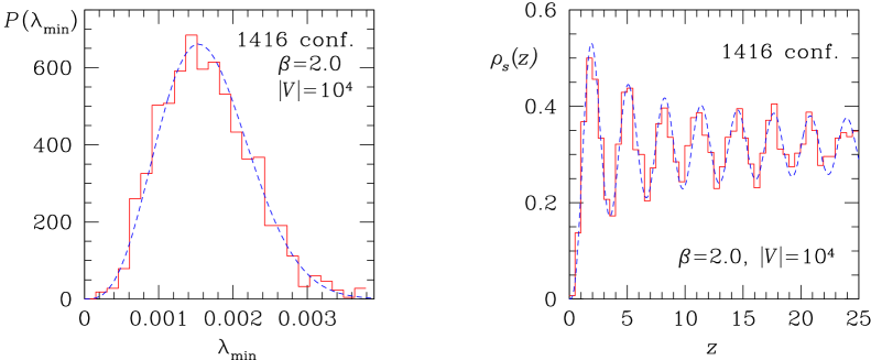
Figure 3: Distribution of the smallest eigenvalue (left) and microscopic spectral density (right) of the QCD Dirac operator. The histograms represent lattice data in quenched SU(2) with staggered fermions on a $10^{4}$ lattice using $\beta=4/g^{2}=2.0$ (not to be confused with the Dyson index $\beta$). The dashed curves are the parameter-free RMT predictions. Taken from Ref. Berb98 with kind permission from the American Physical Society.

The result for $\rho_{s}(z)$ for the chGUE (appropriate for QCD with three and more colors) and gauge fields with topological charge $\nu$ reads Verb93 ; Verb94a

$$\rho_{s}(z)=\frac{z}{2}\left[J_{N_{f}+|\nu|}^{2}(z)-J_{N_{f}+|\nu|+1}(z)J_{N_{f}+|\nu|-1}(z)\right]\>,$$ (101)

where $J$ denotes the Bessel function. The results for the chGSE and the chGOE are more complicated. Lattice QCD data agree with RMT predictions as seen in Fig. 3 which represents results corresponding to the chGSE.

QCD at nonzero temperature and chemical potential

Random-matrix models can also be used to model and analyze generic properties of the chiral symmetry restoration phase transition at finite temperature or finite baryon chemical potential $\mu$. For example, the effect of the chemical potential can be described by the non-Hermitian deformation (24) of the chGUE. The eigenvalues of such a matrix are not constrained to lie on the real axis. The quantity that signals chiral symmetry breaking is the discontinuity (a cut) of the averaged resolvent $\langle G(z)\rangle$ at $z=0$. One can calculate $\langle G(z)\rangle$ in a theory with $n\neq 0$, which corresponds to QCD with $n$ species of quarks. There is a critical value of $\mu$ above which $\langle G(z)\rangle$ becomes continuous at $z=0$, and, therefore, chiral symmetry is restored. In lattice Monte Carlo the problem of calculating the partition function and expectation values such as $\langle G(z)\rangle$ at finite $\mu$, which are of a paramount interest to experiment, is still unresolved. The difficulty lies in the fact that the determinant of the Dirac matrix is complex and cannot be used as part of the probabilistic measure to generate configurations using the Monte Carlo method. For this reason, exploratory simulations at finite $\mu$ have only been done in the quenched approximation in which the fermion determinant is ignored, $n=0$. The results of such simulations were in a puzzling contradiction with physical expectations: The transition to restoration of chiral symmetry occurs at $\mu=0$ in the quenched approximation.

The chiral random matrix model at $\mu\neq 0$ allows for a clean analytical explanation of this behavior, since one can calculate $\langle G(z)\rangle$ both at $n=0$ and $n\neq 0$. (As before, the number of replicas is denoted by $n$.) The behavior of $\langle G(z)\rangle$ at $n=0$ and $n\neq 0$ is drastically different. While at $n\neq 0$ the non-analyticities of $\langle G(z)\rangle$ come in the form of one-dimensional cuts, for $n=0$ they form two-dimensional regions, similar to the Ginibre circle in the case of the non-Hermitian GUE. This means that the $n=0$ (quenched) theory is not a good approximation to the $n\neq 0$ (full) theory at finite $\mu$, when the Dirac operator is non-Hermitian. The quenched theory is an approximation (or, the $n\to 0$ limit) of a theory with the determinant of the Dirac operator replaced by its absolute value, which has different properties at finite $\mu$ Step96 .

Quantum gravity in two dimensions.

In all cases we have discussed so far, the random-matrix model was constructed for the Hamiltonian (or a similar operator) of the system, and the universal properties were independent of the distribution of the random matrix. In contrast, in quantum gravity the elementary fields are replaced by matrices, and the details of the matrix potential do influence the results. For a recent review we refer to zinn .

Two dimensional quantum gravity is closely related to string theory. The elementary degrees of freedom are the positions of the string in $d$ dimensions. The action, $S$, of the theory involves kinematic terms and the metric. The partition function, $Z$, is then given as a path integral of $\exp(-S)$ over all possible positions and metrics. The string sweeps out two-dimensional surfaces, and $Z$ can be computed in a so-called genus expansion, i.e., as a sum over all possible topologies of these surfaces. This is typically done by discretizing the surfaces. One can then construct dual graphs by connecting the centers of adjacent polygons (with $n$ sides). These dual graphs turn out to be the Feynman diagrams of a $\varphi^{n}$-theory in zero dimensions which can be reformulated in terms of a matrix model. The partition function of this model is given by

$$Z=\int{\cal D}M\>e^{-N{\rm tr\>}v(M)}\quad{\rm with}\quad v(M)=\sum_{n\geq 1}g_{n}M^{n}\>,$$ (102)

where the $M$ are Hermitian matrices of dimension $N$ and the $g_{n}$ are coupling constants involving appropriate powers of the cosmological constant. The mathematical methods used to deal with the matrix model of quantum gravity are closely related to those employed in RMT, giving rise to a useful interchange between the two areas.

Acknowledgements. We are grateful for the numerous discussions with collaborators and friends this work has benefited from. Peter Sellinger is acknowledged for the potrace software that greatly improved the quality of Fig. 1 and Fig. 2. This work was partially supported by NSF grant PHY97-22101 (MAS), U.S. DOE grant DE-FG-88ER40388 (JJMV) and by the Deutsche Forschungsgemeinschaft (TW).

References

- (1) J. Wishart, Biometrika 20 (1928) 32.
- (2) E.P. Wigner, Ann. Math. 62 (1955) 548.
- (3) F.J. Dyson, J. Math. Phys. 3 (1962) 140, 157,166, 1191, 1199.
- (4) C.E. Porter, Statistical Theory of Spectra: Fluctuations, Academic Press, New York 1965.
- (5) M.L. Mehta, Random matrices, 2nd ed. (Academic Press, San Diego, 1991).
- (6) T. Guhr, A. Müller-Groeling, and H.A. Weidenmüller, Phys. Rep. 299 (1998) 189.
- (7) J.J.M. Verbaarschot, Phys. Rev. Lett. 72 (1994) 2531.
- (8) R. Gade, Nucl. Phys. B398 (1993) 499.
- (9) A. Altland, M.R. Zirnbauer, Phys. Rev. Lett. 76 (1996) 3420.
- (10) M.R. Zirnbauer, J. Math. Phys. 37 (1996) 4986.
- (11) R. Oppermann, Physica A167 (1990) 301.
- (12) L.K. Hua, Harmonic Analysis , American Mathematical Society 1963.
- (13) J.Ginibre, J.Math.Phys 6 (1965) 440.
- (14) J.J.M. Verbaarschot, H.A. Weidenmüller, and M.R. Zirnbauer, Phys. Rep. 129 (1985) 367.
- (15) K.B. Efetov, Phys. Rev. Lett. 79 (1997) 491; Phys. Rev. B 56 (1997) 9630.
- (16) Y.V. Fyodorov, B.A. Khoruzhenko and H.-J. Sommers, Phys. Rev. Lett. 79 (1997) 557.
- (17) M.A. Stephanov, Phys. Rev. Lett. 76 (1996) 4472.
- (18) G. Hackenbroich and H.A. Weidenmüller, Phys. Rev. Lett. 7 (1995) 4118.
- (19) G. Akemann, P. Damgaard, U. Magnea and S. Nishigaki, Nucl. Phys. B 487 (1997) 721.
- (20) E.V. Shuryak and J.J.M. Verbaarschot, Nucl. Phys. A 560 (1993) 306.
- (21) S.M. Nishigaki, P.H. Damgaard, and T. Wettig, Phys. Rev. D 59 (1998) 087704.
- (22) P.W. Anderson, Phys. Rev. 109 (1958) 1492.
- (23) O. Bohigas, M.-J. Giannoni, and C. Schmit, Phys. Rev. Lett. 52 (1984) 1.
- (24) A. Selberg, Norsk Mat. Tidsskr. 26 (1944) 71.
- (25) J.J.M. Verbaarschot, Phys. Lett. B 329 (1994) 351.
- (26) K. Aomoto, SIAM J. Math. Anal. 18 (1987) 545.
- (27) J. Kaneko, SIAM J. Math. Anal. 24 (1993) 1086.
- (28) K. Efetov, Adv. Phys. 32 (1983) 53.
- (29) K. Efetov, Supersymmetry in Disorder and Chaos, Cambridge University Press, Cambridge 1997.
- (30) T. Guhr, J. Math. Phys. 32 (1991) 336; T. Guhr and T. Wettig, J. Math. Phys. 37 (1996) 6395.
- (31) S.F. Edwards and P.W. Anderson, J. Phys. F: Met. Phys. 5 (1975) 965.
- (32) J.J.M. Verbaarschot and M.R. Zirnbauer, J. Phys. A: Math. Gen. 17 (1985) 1093.
- (33) D. Agassi, H.A. Weidenmüller and G. Mantzouranis, Phys. REp. C (1975) 145.
- (34) V.L. Girko, Theory of random determinants, Kluwer Academic Publishers, Dordrecht 1990.
- (35) H.J. Sommers, A. Crisanti, H. Sompolinski and Y. Stein, Phys. Rev. Lett. 60 (1988) 1895.
- (36) J. Feinberg and A. Zee, Nucl. Phys. B 504 (1998) 579.
- (37) O. Bohigas, R.U. Haq, and A. Pandey, in Nuclear data for science and technology, ed. K.H. Böchhoff (Reidel, Dordrecht, 1983) 809.
- (38) D. Wintgen, Phys. Rev. Lett. 58 (1987) 1589; D. Wintgen and H. Friedrich, Phys. Rev. A 35 (1987) 1464.
- (39) H. Friedrich and D. Wintgen, Phys. Rep. 183 (1989) 37.
- (40) M.C. Gutzwiller, Chaos in Classical and Quantum Mechanics (Springer, New York, 1990).
- (41) C.M. Marcus, A.J. Rimberg, R.M. Westervelt, P.F. Hopkins, and A.C. Gossard, Phys. Rev. Lett. 69 (1992) 506.
- (42) C.W.J. Beenakker, Rev. Mod. Phys. 69 (1997) 731.
- (43) D.J. Thouless, Phys. Rep. 13 (1974) 93.
- (44) S. Washburn and R.A. Webb, Adv. Phys. 35 (1986) 375.
- (45) S. Deus, P.M. Koch, and L. Sirko, Phys. Rev. E 52 (1995) 1146.
- (46) H. Alt, H.D. Gräf, R. Hofferbert, C. Rangacharyulu, H. Rehfeld, A. Richter, P. Schardt, and A. Wirzba, Phys. Rev. E 54 (1996) 2303.
- (47) C. Ellegaard, T. Guhr, K. Lindemann, H.Q. Lorensen, J. Nygård, and M. Oxborrow, Phys. Rev. Lett. 75 (1995) 1546.
- (48) H.L. Montgomery, Proc. Symp. Pure Maths. 24 (1973) 181.
-
(49)
A.M. Odlyzko, Math. Comput. 48 (1987) 273;
http://www.research.att.com/~amo/unpublished/zeta.10to20.1992.ps. - (50) H. Leutwyler and A.V. Smilga, Phys. Rev. D 46 (1992) 5607.
- (51) J. C. Osborn, D. Toublan and J. J. M. Verbaarschot, Nucl. Phys. B 540, 317 (1999).
- (52) M.A. Halasz and J.J.M. Verbaarschot, Phys. Rev. Lett. 74 (1995) 3920; R. Pullirsch, K. Rabitsch, T. Wettig, and H. Markum, Phys. Lett. B 427 (1998) 119.
- (53) J.J.M. Verbaarschot and I. Zahed, Phys. Rev. Lett. 70 (1993) 3852.
- (54) M.E. Berbenni-Bitsch, S. Meyer, A. Schäfer, J.J.M. Verbaarschot, and T. Wettig, Phys. Rev. Lett. 80 (1998) 1146.
- (55) P. Di Francesco, P. Ginsparg, and J. Zinn-Justin, Phys. Rep. 254 (1995) 1.