Semi-superfluid strings in High Density QCD

Abstract

We show that topological superfluid strings/vortices with flux tubes exist in the color-flavor locked (CFL) phase of color superconductors. Using a Ginzburg-Landau free energy we find the configurations of these strings. These strings can form during the transition from the normal phase to the CFL phase at the core of very dense stars. We discuss an interesting scenario for a network of strings and its evolution at the core of dense stars.

I Introduction

Color superconductivity is expected to be the ground state for high baryon chemical potential $\displaystyle\mu$ and low temperatures BL . It is believed that such a state of matter may exist at the core of very dense stars. To find any signature of its existence, it is important to study various properties of the color superconducting phase. When all the quarks are massless, there are superconducting phases, namely the color-flavor locked (CFL) and the 2SC phasesBL . In the CFL phase, all quark flavors take part in the condensation, but in the 2SC phase, one quark does not participate in the condensation. With realistic values of quark masses and charge neutrality conditions, the CFL phase gets modified to phases known as mCFL, dSC taeko , uSC uSC , gCFL, g2SC Alford:2003fq ; Shovkovy:2003uu , and FFLO phases loff ; Alford:2000ze etc. One of the interesting properties of a color superconductor is that it is also a superfluid. This is because apart from local symmetries, such as $\displaystyle SU(3)_{C}$ of color symmetry and $\displaystyle U(1)_{EM}$ of electromagnetism, certain global symmetries are also spontaneously broken in the superconducting phase. The global symmetries spontaneously broken in the superconducting phase are $\displaystyle SU(3)_{F}$ (the flavor symmetry) and $\displaystyle U(1)_{B}$ (the baryon number symmetry). One expects defect solutions such as flux tubes or vortices to be present in the superconductor since it is both a superconductor and a superfluid. Recently there have been lots of studies of superfluid vortices ZH ; iida-baym and flux tubes iida in the color flavor locked (CFL) phase and in the 2SC phase Bs . In these studies, superfluid vortices are topologically stable. The flux tubes studied so far are not topological and it is not clear if they are stable at all.

All the topological string solutions like vortices or flux tubes are due to and are related to the existence of nontrivial loops (NNL’s) in the order parameter space ($\displaystyle OPS$). An $\displaystyle OPS$ is the set of all possible values of the order parameter ($\displaystyle OP$) which is the diquark condensate in this case. Each NNL in the $\displaystyle OPS$ corresponds to nontrivial defect solutions in the superconducting phase. Previous studies have considered NNL’s in the $\displaystyle OPS$ which are generated only by the baryon number charge ZH ; iida-baym . However when symmetry groups such as color, flavor and baryon number are spontaneously broken, one can have other NNL’s. There are NNL’s in the $\displaystyle OPS$ which are generated partly by the baryon number and partly by other non-abelian color or flavor generators bal . These loops give rise to non-abelian strings. These string defects have been studied previously in the context of broken chiral symmetry in the framework of the linear sigma model bal-digal . In this work we consider the non-abelian defects in the color superconducting phase. We include the effects of gauge fields which result in flux tubes. These flux tubes are unlike those in ordinary superconductors. The energy per unit length of the string behaves like that of a superfluid vortex. This is why we call these non-abelian flux tubes as semi-superfluid strings. In this work we consider the semi-superfluid strings in the CFL phase. We will argue that these defects and superfluid vortices are possible in the dSC, uSC and mCFL phases. In order that the flux tubes are dynamically stable, the color superconductor must be type II. For asymptotic values of the chemical potential $\displaystyle\mu$, the color superconductor is type I, but for intermediate values of $\displaystyle\mu$ it can be type II ren ; iida-baym .

This paper is organized as follows. In the next section, we discuss the Ginzburg-Landau free energy and discuss the nontrivial loops in the $\displaystyle OPS$ which give rise to the non-abelian string defects. Section III will contain numerical results for the configuration of string defects in the CFL phase. In section IV we discuss a possible scenario for the string network and its evolution at the core of a very dense star. In Section IV, we present our conclusions.

II Ginzburg-Landau free energy and the $\displaystyle OPS$

In the superconducting phase the dominant pairing channel consists of two quarks of the same helicity. We will denote the corresponding order parameters by $\displaystyle\Phi_{L}$ and $\displaystyle\Phi_{R}$. $\displaystyle\Phi_{L,R}$ are $\displaystyle 3\times 3$ matrices transforming by the $\displaystyle\bar{3}$ representation of $\displaystyle SU(3)_{C}$ and $\displaystyle SU(3)_{L,R}$. One can argue that a semi-superfluid string has the same winding number for both $\displaystyle\Phi_{L}$ and $\displaystyle\Phi_{R}$. In our calculation we assume that $\displaystyle\Phi_{L}=\Phi_{R}\equiv\Phi$. The Ginzburg-Landau(GL) free energy is a function of $\displaystyle\Phi$. In the weak coupling and in the chiral limit it is given by GR iida-baym

$$\displaystyle\Gamma \displaystyle= \displaystyle{1\over 4}G_{ij}^{a}G_{ij}^{a}+{1\over 4}F_{ij}^{EM}F_{ij}^{EM}+2\kappa_{T}{\rm{tr}}({\vec{D}}\Phi)^{{\dagger}}({\vec{D}}\Phi)+\bar{\alpha}{\rm{tr}}(\Phi^{{\dagger}}\Phi)+\beta_{1}({\rm{tr}}\Phi^{{\dagger}}\Phi)^{2}+\beta_{2}{\rm{tr}}(\Phi^{{\dagger}}\Phi)^{2}$$ (1)

If the static electromagnetic gauge field is $\displaystyle\vec{A}^{EM}$ and the static color gauge fields are $\displaystyle\vec{A}^{a}$, $\displaystyle a=1,...,8,$ the covariant derivatives and field strengths are

$$\displaystyle\vec{D}\Phi \displaystyle= \displaystyle{\vec{\nabla}}\Phi-ig{\vec{A}^{a}T^{a}}\Phi-ie{\vec{A}^{EM}T^{EM}}\Phi,$$

$$\displaystyle G_{ij}^{a} \displaystyle= \displaystyle\partial_{i}A_{j}^{a}-\partial_{j}A_{i}^{a}+gf_{abc}A_{i}^{b}A_{j}^{c},$$

$$\displaystyle F_{ij}^{EM} \displaystyle= \displaystyle\partial_{i}A_{j}^{EM}-\partial_{j}A_{i}^{EM}.$$ (2)

Now if the field is $\displaystyle\Phi=\Phi_{L}(\Phi_{R})$ then the corresponding flavor symmetry group is $\displaystyle SU(3)_{F}=SU(3)_{L}(SU(3)_{R})$. Under the element $\displaystyle\{V_{C},V_{F},e^{i\alpha_{B}}\}\in SU(3)_{C}\times SU(3)_{F}\times U(1)_{B}$, the diquark condensate transforms as

$$\displaystyle\Phi\to V_{F}\Phi V_{C}^{T}e^{i\alpha_{B}}$$ (3)

where $\displaystyle V_{F}\in\rm{(the~{}\bar{3}~{}represenation~{}of)}SU(3)_{F}$, $\displaystyle V_{C}\in\rm{(the~{}\bar{3}~{}represenation~{}of)}SU(3)_{C}$ and $\displaystyle e^{i\alpha_{B}}\in U(1)_{B}$. However from Eq.(3), we see that the group of elements $\displaystyle\{(z_{1},z_{1}^{-1}z_{2}^{-1},z_{2}):z_{1},z_{2}={\rm a~{}cube~{}root~{}of~{}unity}\}=Z_{3}\times Z_{3}$ leaves $\displaystyle\Phi$ invariant. So the symmetry group of the free energy $\displaystyle\Gamma$ is

$$G={SU(3)_{C}\times SU(3)_{F}\times U(1)_{B}\over Z_{3}\times Z_{3}}.$$ (4)

In the symmetric or QGP phase, the diquark condensate vanishes and so is invariant under the group $\displaystyle G$. On the other hand $\displaystyle\Phi$ is non-zero in the superconducting phase. As a result a smaller group ($\displaystyle H\in G$) of transformations keeps $\displaystyle\Phi$ invariant. The symmetry group $\displaystyle H$ depends on the form of $\displaystyle\Phi$ and thereby on the state of the superconducting phase.

In the CFL phase the free energy $\displaystyle\Gamma$ is minimized when $\displaystyle\Phi$ is proportional to a constant unitary matrix $\displaystyle U$. So one can write for the minimum energy configuration, $\displaystyle\Phi_{0}$,

$$\Phi_{0}=\eta U$$ (5)

with $\displaystyle\eta$ is a positive real number. For the analysis of the symmetry breaking pattern one can take $\displaystyle\Phi_{0}=\eta\bf{1}$ without loss of generality, where $\displaystyle\bf{1}$ is a $\displaystyle 3\times 3$ identity matrix. The group $\displaystyle SU(3)\times Z_{3}:\{(V,V^{-1}z^{-1},z):z={\rm a~{}cube~{}root~{}of~{}unity},V\in SU(3)\}$ keeps $\displaystyle\Phi_{0}=\eta\bf{1}$ invariant. This set contains all the elements of $\displaystyle Z_{3}\times Z_{3}$ defined above. In order to find the stability group $\displaystyle H\subset G$ of $\displaystyle\Phi_{0}$ we must quotient this set by $\displaystyle Z_{3}\times Z_{3}$. Hence

$$H={SU(3)\times Z_{3}\over Z_{3}\times Z_{3}}.$$ (6)

The symmetry breaking pattern in the transition from normal to CFL phase ($\displaystyle G\to H$) therefore is

$${SU(3)_{C}\times SU(3)_{F}\times U(1)_{B}\over Z_{3}\times Z_{3}}\to{SU(3)\times Z_{3}\over Z_{3}\times Z_{3}}.$$ (7)

Thus the order parameter space $\displaystyle OPS$ for the $\displaystyle\Phi$ is given by,

$$OPS=[SU(3)_{C}\times SU(3)_{F}\times U(1)_{B}]/[SU(3)\times Z_{3}]=U(3)={SU(3)\times U(1)\over Z_{3}}.$$ (8)

The $\displaystyle OPS=U(3)$ allows NNL’s. In the language of homotopy groups, the NNL’s are classified by the first homotopy group $\displaystyle\pi_{1}(OPS)$. In this case,

$$\displaystyle\pi_{1}(OPS)=Z.$$ (9)

We now explain its features.

$\displaystyle U(3)$ allows for non-abelian vortices. We can see this as follows. A nontrivial closed loop in $\displaystyle U(3)$ can be described by a curve in $\displaystyle SU(3)\times U(1)$ beginning at identity which becomes closed on quotienting by $\displaystyle Z_{3}$. Consider the curve from $\displaystyle(\bf{1},\bf{1})$ to $\displaystyle(e^{i2\pi/3},e^{-i2\pi/3})$ in $\displaystyle SU(3)\times U(1)$. In the $\displaystyle SU(3)$ part, only the end points of this curve matter to determine the homotopy class of this curve. In the $\displaystyle U(1)$ part, it is the curve $\displaystyle\{e^{i\varphi}:0\leq\varphi\leq-2\pi/3\}$ from $\displaystyle\bf{1}$ to $\displaystyle e^{-i2\pi/3}$ in the anticlockwise direction. The $\displaystyle SU(3)$ part of this curve is nontrivial. In $\displaystyle U(3)$ then, it is a nontrivial non-abelian closed loop $\displaystyle l$. It is the generator of $\displaystyle Z$ in Eq.(9). If $\displaystyle[l]$ is the homotopy class of this loop, $\displaystyle[l]^{3}$ is associated with a closed loop in $\displaystyle SU(3)$ and $\displaystyle U(1)$. The closed loop in $\displaystyle SU(3)$ can be deformed to a point. Hence $\displaystyle[l]^{3}$ is a NNL in $\displaystyle U(1)$ and corresponds to the abelian superfluid vortices studied in ref.ZH . The elementary non-abelian vortices can be associated with $\displaystyle[l]$ or $\displaystyle[l]^{-1}$. Any non-abelian vortex is associated with $\displaystyle[l][l]^{3k}$ or $\displaystyle[l]^{2}[l]^{3k}$ for $\displaystyle k\in Z$.

Now we construct the loops in the $\displaystyle OPS$. We consider two loops, one in the homotopy class of $\displaystyle[l]$ and the other in the homotopy class $\displaystyle[l^{\prime}]=[l]^{-2}$. The projections of these loops in the $\displaystyle SU(3)$ part of the $\displaystyle OPS$ are same. The projections of loops $\displaystyle l$ and $\displaystyle l^{\prime}$ in $\displaystyle U(1)_{B}$ go from identity to $\displaystyle e^{-2\pi i/3}$ in the anti-clockwise and clock-wise directions respectively. The latter explicitly is $\displaystyle\{e^{i\varphi}:0\leq\varphi\leq 4\pi/3\}$. In $\displaystyle U(1)_{B}$ they are generated by the baryon charge,

$$\displaystyle Q_{B}={2\over 3}\bf{1}.$$ (10)

The loops $\displaystyle l$ and $\displaystyle l^{\prime}$ are parameterized in $\displaystyle U(1)_{B}$ as

$$\displaystyle e^{-i\alpha Q_{B}/2},~{}~{}e^{i\alpha Q_{B}}$$ (11)

where the parameter $\displaystyle\alpha$ varies from $\displaystyle 0$ to $\displaystyle 2\pi$. Both these loops start from identity and end at $\displaystyle e^{4\pi i/3}$ in $\displaystyle U(1)_{B}$.

Now let us discuss the projection of the loops $\displaystyle l$ and $\displaystyle l^{\prime}$ on the individual groups $\displaystyle SU(3)_{C}$ and $\displaystyle SU(3)_{F}$. Note that the $\displaystyle U(1)_{EM}$ is a subgroup of $\displaystyle SU(3)_{F}$. The generator $\displaystyle T^{EM}$ of $\displaystyle U(1)_{EM}$ in the $\displaystyle(ds,su,ud)$ basis is given by

$$\displaystyle T^{EM}={1\over 3}\left(\begin{array}[]{ccc}-2&0&0\\ 0&1&0\\ 0&0&1\end{array}\right)$$ (13)

which is linear combination of the generators $\displaystyle S^{3}$ and $\displaystyle S^{8}$ of $\displaystyle SU(3)_{F}$. So a curve generated by $\displaystyle T^{EM}$ lies entirely in $\displaystyle SU(3)_{F}$. To simplify the matter we work in a basis of generators such that $\displaystyle T^{8}(S^{8})$ of $\displaystyle SU(3)_{c}(SU(3)_{F})$ have the same matrix representation

$$\displaystyle{1\over 2\sqrt{3}}\left(\begin{array}[]{ccc}-2&0&0\\ 0&1&0\\ 0&0&1\end{array}\right)$$ (16)

as in ref.ren . A path from $\displaystyle(1,1)$ to $\displaystyle e^{2\pi i/3}(1,1)$ in $\displaystyle SU(3)_{C}\times SU(3)_{F}$ can be generated by $\displaystyle T^{EM}$ or $\displaystyle T^{8}$ a linear combination of them. The projection of this curve on $\displaystyle SU(3)_{C}$ and on $\displaystyle SU(3)_{F}$ can be different. For example the projection of this curve can go from $\displaystyle\bf{1}$ to $\displaystyle e^{2\pi i/3}$ in $\displaystyle SU(3)_{C}$ and be just a point in $\displaystyle SU(3)_{F}$ or vice-versa. Topologically there is no difference between these different possibilities. However dynamically they are different. When the projection in $\displaystyle SU(3)_{C}$ is from $\displaystyle\bf{1}$ to $\displaystyle e^{2\pi i/3}$ and just a point in $\displaystyle SU(3)_{F}$ the resulting string configuration will be made of only color fields with $\displaystyle g{\sqrt{3}\over 2}{\bar{\Phi}^{8}}={2\pi}$. On the other hand if the projection in $\displaystyle SU(3)_{F}$ is from $\displaystyle\bf{1}$ to $\displaystyle e^{2\pi i/3}$ and is just a point in $\displaystyle SU(3)_{C}$, the resulting string configuration will be made of only ordinary magnetic field with $\displaystyle e{\bar{\Phi}^{EM}}={2\pi}$. But in CFL there is a mixing between $\displaystyle A^{EM}$ and $\displaystyle A^{8}$ into the following new gauge fields mixing ,

$$\displaystyle A_{X}=\cos\zeta A^{EM}+\sin\zeta A^{8}$$

$$\displaystyle A_{\tilde{Q}}=-\sin\zeta A^{EM}+\cos\zeta A^{8}$$ (18)

where $\displaystyle A_{X}$ is massive and $\displaystyle A_{\tilde{Q}}$ is massless. $\displaystyle\zeta$ depends on the couplings as follows:

$$\cos\zeta=\sqrt{e^{2}\over e^{2}+3g^{2}/4}.$$ (19)

Because of the mixing between the gauge fields a path from $\displaystyle(1,1)$ to $\displaystyle e^{2\pi i/3}(1,1)$ in $\displaystyle SU(3)_{C}\times SU(3)_{F}$ has projection both in $\displaystyle SU(3)_{F}$ and $\displaystyle SU(3)_{C}$ for the minimum energy string configuration. As a result for minimum energy, the sum of the ordinary and color magnetic flux should satisfy

$$\displaystyle(e{\bar{\Phi}^{EM}})+g{\sqrt{3}\over 2}{\bar{\Phi}^{8}}=g_{x}\bar{\Phi}^{X}=\pm 2\pi$$ (20)

where $\displaystyle\bar{\Phi}^{X}$ is the magnetic flux of the massive gauge field $\displaystyle A^{X}$ and $\displaystyle g_{x}=\sqrt{e^{2}+3g^{2}/4}$. Note that even though the minimum energy configuration has a flux both of ordinary and color magnetic fields, a configuration with only ordinary magnetic flux can still be stable because of flux conservation.

We mention here that previous studies iida have considered the flux tube of the $\displaystyle A^{X}$ field. This flux tube is analogous to the electroweak string. Unlike our case these solutions correspond to a closed loop in the $\displaystyle SU(3)$ part of the $\displaystyle OPS$ and are not topologically stable. Their counterparts in the electroweak theory have been extensively studied vachaspati for stability. The results show that when the weak gauge coupling is larger than the abelian gauge coupling the solutions are unstable against expanding of the core of the string. For the same reason the flux tube iida considered previously in CFL will be unstable because the strong coupling constant is an order of magnitude larger than the electromagnetic coupling.

We expect that in the gCFL phase also there will be semi-superfluid strings since the symmetry breaking pattern and the $\displaystyle OPS$ are same as that of CFL case. In the mCFL phase we expect that the loops considered in the above discussion remain non-trivial. Since different components of $\displaystyle\Phi$ have different mass in this case the core structure of the defect will be different from the case when quark masses are degenerate and are zero. The abelian loops $\displaystyle[l]^{3k}$ as well as non-abelian loops $\displaystyle[l][l]^{3k}$ and $\displaystyle[l]^{2}[l]^{3k}$ still remain when quark masses are finite. Because of spontaneous breaking of $\displaystyle U(1)_{B}$ the $\displaystyle OPS$ always contains a $\displaystyle U(1)$. The effect of non-zero masses only changes part of the $\displaystyle OPS$ which is generated by the nonabelian generators. However this change does not affect the above non-abelian NNS’s as long as the nonabelian generator of this loops $\displaystyle T^{8}$ is not explicitly broken. So there should be non-abelian strings in the mCFL phase. The same arguments can be made about the dSC and uSC phase. For the 2SC and g2SC cases the situation is similar to the electroweak case. As the condensate has only one nonvanishing component, the loops generated by $\displaystyle Q_{B}$ and $\displaystyle T^{8}$ are same and hence will lie in $\displaystyle SU(3)_{C,F}$. So one will not have any stable topological string solution in the 2SC and g2SC phases.

III Field Equations and Numerical solutions for NA Semi-superfluid strings

In this section we consider the $\displaystyle l$ and $\displaystyle l^{\prime}$ in the $\displaystyle OPS$ and derive the action and the field equation for the semi-superfluid strings. As we mentioned above, because of the mixing between $\displaystyle\vec{A}^{EM}$ and $\displaystyle\vec{A}_{8}$, the NNL’s will have projections in both $\displaystyle SU(3)_{F}$ and $\displaystyle SU(3)_{C}$. In the following, we will denote the generator corresponding to the massive gauge field $\displaystyle A_{X}$ by $\displaystyle A$. To simplify the notations we denote $\displaystyle T^{EM}$ by $\displaystyle T$ in the following. The loops $\displaystyle l$ and $\displaystyle l^{\prime}$ are parameterized by

$$\displaystyle M_{1}(\alpha)=\eta e^{i\alpha({T-Q_{B}/2})}=\eta\left(\begin{array}[]{ccc}e^{-i\alpha}&0&0\\ 0&1&0\\ 0&0&1\end{array}\right),$$ (22)

$$\displaystyle M_{2}(\alpha)=\eta e^{i\alpha({T+Q_{B}})}=\eta\left(\begin{array}[]{ccc}1&0&0\\ 0&e^{i\alpha}&0\\ 0&0&e^{i\alpha}\end{array}\right)$$ (24)

with a constant $\displaystyle\eta$.

The projection of $\displaystyle\{M_{1}(\alpha):\alpha\in[0,2\pi]\}$ in $\displaystyle SU(3)$ goes from $\displaystyle I$ to the center element $\displaystyle e^{2\pi i/3}$ while the projection in $\displaystyle U(1)_{B}$ goes from $\displaystyle I$ to $\displaystyle e^{-2\pi i/3}$. The second loop $\displaystyle\{M_{2}(\alpha):\alpha\in[0,2\pi]\}$ is the same as $\displaystyle M_{1}(\alpha)$ except the path in $\displaystyle U(1)_{B}$ is covered with the reversed orientation.

The minimum energy configuration strings are associated with $\displaystyle M_{1}(\alpha)$ or $\displaystyle M_{2}(\alpha)$. To keep the energy contribution from the covariant derivative to its minimum, only the massive gauge field $\displaystyle A$ is excited. Assuming that the string is along the $\displaystyle z$-axis and is cylindrically symmetrical around it, the $\displaystyle\Phi$ configuration for the string (corresponding to $\displaystyle M_{1}(\alpha)$ with $\displaystyle\alpha=\theta$, $\displaystyle\theta$ being the polar angle of the position vector on the $\displaystyle xy$-plane) is given by

$$\displaystyle\Phi(r,\theta) \displaystyle= \displaystyle\left(\begin{array}[]{ccc}\eta f(r)e^{-in\theta}&0&0\\ 0&\psi_{1}(r)&0\\ 0&0&\psi_{2}(r)\end{array}\right)\equiv\left(\begin{array}[]{ccc}\phi(r,\theta)&0&0\\ 0&\psi_{1}(r)&0\\ 0&0&\psi_{2}(r)\end{array}\right)$$ (27)

To simplify our calculations we assume that $\displaystyle\psi_{1,2}(r)=\eta$. The string configuration with the lowest energy will have some $\displaystyle r$ dependent profile for $\displaystyle\psi_{1,2}(r)$. Near the core of the string $\displaystyle\psi_{1,2}$ will have values slightly larger than $\displaystyle\eta$ due to coupling with the $\displaystyle\phi$ field and the gauge fields ren . Far from the core of the string where $\displaystyle r\to\infty$, $\displaystyle\psi_{1,2}(r)$ must be equal to $\displaystyle\eta$ but without any nontrivial winding like the $\displaystyle\phi$ field.

The finiteness of the potential energy part of the free energy (Eq.(1)) requires that $\displaystyle f(r\to\infty)=1$. The kinetic energy part of the free energy can be minimized by an appropriate choice of the gauge fields $\displaystyle\vec{A}$. Since the string is cylindrically symmetrical, the phase varies only in the $\displaystyle\theta$ direction in the $\displaystyle x,y$ plane, so only the $\displaystyle A_{\theta}$ will be non-zero. The total static free energy corresponding to the loop $\displaystyle\{M_{1}(\alpha),\alpha\in[0,2\pi]\}$ with $\displaystyle\phi=\eta f(r)e^{-in\theta}$ is given by

$$\displaystyle\Gamma(\Phi,\vec{A})=2\kappa_{T}|(\vec{\partial}+{i2g_{x}\over 3}\vec{A})\phi|^{2}+{4g_{x}^{2}\kappa_{T}\eta^{2}\over 9}A^{2}+\frac{1}{4}(\partial_{\mu}A_{\nu}-\partial_{\nu}A_{\mu})^{2}$$

$$\displaystyle+{\bar{\alpha}}(|\phi|^{2}+2\eta^{2})+\beta(2\phi^{4}+4\eta^{2}\phi^{2}+6\eta^{4}).$$ (29)

The above free energy is minimized if, at a large distance $\displaystyle r$ from the string, $\displaystyle A_{\theta}$ is a pure gauge field. This implies the following form for the gauge field $\displaystyle A_{\theta}$:

$$\displaystyle A_{\theta}={\xi\gamma(r)\over r},\gamma(r\to\infty)=1.$$ (30)

Now the covariant derivative in the $\displaystyle\theta$ direction is given by

$$\displaystyle D_{\theta}\Phi=\partial_{\theta}\Phi-ig_{x}A_{\theta}T\Phi \displaystyle= \displaystyle\eta\left(\begin{array}[]{ccc}(-i{n\over r}+{2ig_{x}\xi\over 3r})e^{-in\theta}&0&0\\ 0&-{ig_{x}\xi\over 3r}&0\\ 0&0&-{ig_{x}\xi\over 3r}\end{array}\right).$$ (32)

The gradient energy density from the variation of the fields along the $\displaystyle\theta$ direction is given by

$$\displaystyle|D_{\theta}\Phi|^{2}={\eta^{2}\over 9r^{2}}\left[(3n-2g_{x}\xi)^{2}+2(g_{x}\xi)^{2}\right]$$ (34)

which is minimized by $\displaystyle g_{x}\xi=1$ for $\displaystyle n=1$. So the gauge field $\displaystyle A_{\theta}$ takes the form

$$\displaystyle A_{\theta}={\gamma(r)\over g_{x}r}.$$ (35)

It is important to note that the gauge field reduces the gradient energy by $\displaystyle{1\over 3}$ for the string configuration corresponding to loop $\displaystyle M_{1}(\theta)$.

The Euler-Lagrange equations for $\displaystyle\Phi$ and the gauge field $\displaystyle A$ respectively are

$$\displaystyle\partial_{\mu}\frac{\delta\Gamma}{\delta(\partial\phi^{*})}-\frac{\delta\Gamma}{\delta\phi^{*}} \displaystyle= \displaystyle 2\kappa_{T}(\partial_{\mu}+{2ig_{x}\over 3}A_{\mu})(\partial_{\mu}+{2ig_{x}\over 3}A_{\mu})\phi-(\bar{\alpha}+4\beta\eta^{2})\phi-4\beta|\phi|^{2}\phi=0,$$ (36)

$$\displaystyle\partial_{\mu}\frac{\delta\Gamma}{\delta(\partial A_{\mu})}-\frac{\delta\Gamma}{\delta A_{\mu}} \displaystyle= \displaystyle\partial^{2}A_{\mu}+{4\kappa_{T}ig_{x}\over 3}(\phi^{*}\partial_{\mu}\phi-\phi\partial_{\mu}\phi^{*})-{16\kappa_{T}g_{x}^{2}\over 9}|\phi|^{2}A_{\mu}-{8\kappa_{T}g_{x}^{2}\eta^{2}\over 9}A_{\mu}=0.$$ (37)

The static equations satisfied by $\displaystyle f$ and $\displaystyle\gamma$ are

$$\displaystyle f^{{}^{\prime\prime}}(r)+\frac{1}{r}f^{{}^{\prime}}(r)-\frac{f(r)}{r^{2}}\left({4\gamma(r)\over 3}-1\right)^{2}-\frac{\bar{\alpha}+4\beta\eta^{2}}{2\kappa_{T}}f(r)-\frac{2\beta}{\kappa_{T}}\eta^{2}f^{3}(r)=0,$$ (38)

$$\displaystyle\gamma^{{}^{\prime\prime}}(r)-\frac{1}{r}\gamma^{{}^{\prime}}(r)-8\kappa_{T}g_{x}^{2}\eta^{2}\left({2f^{2}(r)+1\over 9}\right)\gamma(r)+{8\kappa_{T}g_{x}^{2}\eta^{2}f^{2}(r)\over 3}=0.$$ (39)

Now let us consider the string solution for the loop given by $\displaystyle M_{2}(\theta)$. The ansatz for the $\displaystyle\Phi$ field in this case is

$$\displaystyle\Phi(r,\theta) \displaystyle= \displaystyle\left(\begin{array}[]{ccc}\psi(r)&0&0\\ 0&\eta f(r)e^{in\theta}&0\\ 0&0&\eta f(r)e^{in\theta}\end{array}\right).$$ (41)

As in the previous case of the string solution corresponding to the loop $\displaystyle M_{1}$, we assume that $\displaystyle\psi(r)=\eta$ to simplify our calculations. The free energy with $\displaystyle\phi=\eta f(r)e^{in\theta}$ is given by

$$\displaystyle\Gamma(\Phi,\vec{A})=4\kappa_{T}|(\vec{\partial}-{ig_{x}\over 3}\vec{A})\phi|^{2}+{8g_{x}^{2}\kappa_{T}\eta^{2}\over 9}A^{2}+\frac{1}{4}(\partial_{\mu}A_{\nu}-\partial_{\nu}A_{\mu})^{2}$$

$$\displaystyle+{\bar{\alpha}}(2|\phi|^{2}+\eta^{2})+\beta(6\phi^{4}+4\eta^{2}\phi^{2}+2\eta^{4}).$$ (43)

Again since the phase of the condensate depends only on $\displaystyle\theta$, only $\displaystyle A_{\theta}$ is non-zero. To find out the asymptotic form of $\displaystyle A_{\theta}$, we impose the condition that it asymptotically becomes a pure gauge field and also minimizes the gradient energy. The covariant derivative of $\displaystyle\Phi$ is

$$\displaystyle D_{\theta}\Phi=\partial_{\theta}\Phi-ig_{x}A_{\theta}T\Phi \displaystyle= \displaystyle\eta\left(\begin{array}[]{ccc}{2ig_{x}\xi\over 3r}&0&0\\ 0&(i{n\over r}-{ig_{x}\xi\over 3r})e^{in\theta}&0\\ 0&0&(i{n\over r}-{ig_{x}\xi\over 3r})e^{in\theta}\end{array}\right).$$ (45)

The gradient energy density corresponding to the phase variation of $\displaystyle\Phi$ is now given by

$$\displaystyle|D_{\theta}\Phi|^{2}={1\over 9r^{2}}\left[2(3n-g_{x}\xi)^{2}+4(g_{x}\xi)^{2}\right]$$ (47)

which is again minimized by $\displaystyle g_{x}\xi=1$. The reduction in the gradient energy due to the gauge fields is now only by a factor of $\displaystyle{2\over 3}$. The Euler-Lagrange equations for the fields $\displaystyle\phi$ and $\displaystyle\vec{A}$ are

$$\displaystyle\partial_{\mu}\frac{\delta\Gamma}{\delta(\partial\phi^{*})}-\frac{\delta\Gamma}{\delta\phi^{*}} \displaystyle= \displaystyle 4\kappa_{T}(\partial_{\mu}-{ig_{x}\over 3}A_{\mu})(\partial_{\mu}-{ig_{x}\over 3}A_{\mu})\phi-2(\bar{\alpha}+2\beta\eta^{2})\phi-12\beta|\phi|^{2}\phi=0,$$ (48)

$$\displaystyle\partial_{\mu}\frac{\delta\Gamma}{\delta(\partial A_{\mu})}-\frac{\delta\Gamma}{\delta A_{\mu}} \displaystyle= \displaystyle\partial^{2}A_{\mu}-{4\kappa_{T}ig_{x}\over 3}(\phi^{*}\partial_{\mu}\phi-\phi\partial_{\mu}\phi^{*})-{8\kappa_{T}g_{x}^{2}\over 9}|\phi|^{2}A_{\mu}-{16g_{x}^{2}\eta^{2}\over 9}A_{\mu}=0$$ (49)

which simplifies to the following:

$$\displaystyle f^{{}^{\prime\prime}}(r)+\frac{1}{r}f^{{}^{\prime}}(r)-\frac{f(r)}{r^{2}}\left({\gamma(r)\over 3}+1\right)^{2}-\frac{\bar{\alpha}+2\beta\eta^{2}}{2\kappa_{T}}f(r)-\frac{3\beta}{\kappa_{T}}\eta^{2}f^{3}(r)=0,$$ (50)

$$\displaystyle\gamma^{{}^{\prime\prime}}(r)-\frac{1}{r}\gamma^{{}^{\prime}}(r)-8\kappa_{T}g_{x}^{2}\eta^{2}\left({f^{2}(r)+2\over 9}\right)\gamma(r)+{8\kappa_{T}g_{x}^{2}\eta^{2}f^{2}(r)\over 3}=0.$$ (51)

We solve equations (38)-(39) and (50)-(51) numerically to find out the string profile for the two loops $\displaystyle l$ and $\displaystyle l^{\prime}$ respectively. We choose the values of parameters which will correspond to a type II color superconductor. For our calculations we took $\displaystyle g_{x}=2.0$, $\displaystyle\kappa_{T}=0.42$, $\displaystyle\beta=1.26$ and $\displaystyle\eta=100$MeV. The parameter $\displaystyle\bar{\alpha}$ is obtained from the relation $\displaystyle\bar{\alpha}=8\beta\eta^{2}=1.008\times 10^{5}$ MeV². We also use the following relations taeko :

$$\displaystyle\frac{\bar{\alpha}}{\kappa_{T}}\sim\frac{\beta\eta^{2}}{\kappa_{T}}\sim m_{\phi}^{2},$$

$$\displaystyle 2\kappa_{T}g_{x}^{2}\eta^{2}\equiv m_{A}^{2}.$$

For these parameters we have the Higgs mass $\displaystyle m_{\Phi}\sim 245$MeV and the Meissner mass (inverse of the penetration depth) $\displaystyle m_{A}\sim 183$MeV.

The results of our numerical solutions are shown in Fig.1 and Fig.2. Though the figures look similar, the energy of the configurations are very different. One can see that both the $\displaystyle\phi$ and $\displaystyle A$ profiles vary more slowly and reach their asymptotic values at larger $\displaystyle r$ for the string corresponding to the NNL $\displaystyle l^{\prime}$. The NNL $\displaystyle l^{\prime}$ in the $\displaystyle OPS$ travels a longer path in $\displaystyle U(1)_{B}$ which costs larger gradient energy for the semi-superfluid solutions as $\displaystyle U(1)_{B}$ is a global symmetry group.

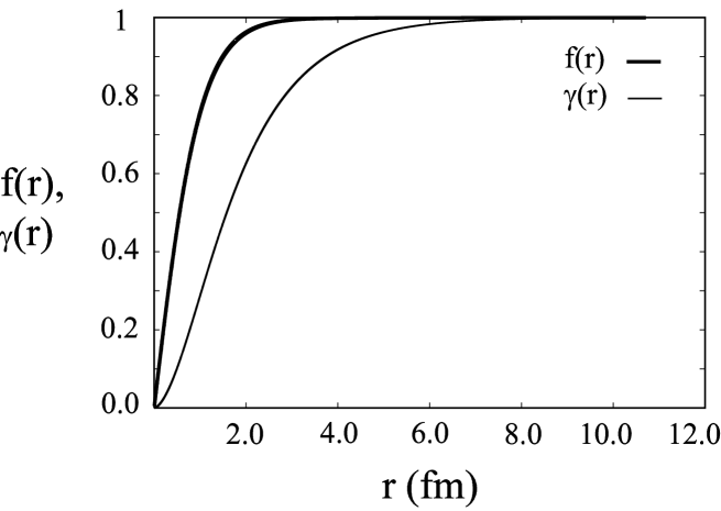
Figure 1: The $\displaystyle f(r)$ and $\displaystyle\gamma(r)$ profiles for the string corresponding to the non-trivial loop $\displaystyle l$.

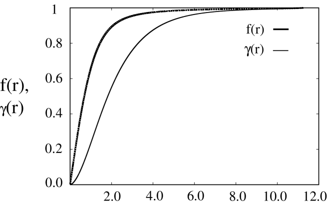
Figure 2: $\displaystyle f(r)$ and $\displaystyle\gamma(r)$ profile for string corresponding to the non-trivial loop $\displaystyle l^{\prime}$

In the profiles of the string, we see that far from the core of the semi-superfluid string, the field is color-flavor locked, i.e. the field is a constant times a $\displaystyle SU(3)$ matrix. However at the core of the string the condensate is not locked.

The NA string corresponding to the loop $\displaystyle M_{1}(\alpha)^{3}$ and a winding number one superfluid string are topologically equivalent. For both these string configurations the energy density is $\displaystyle\sim{3\over r^{2}}$ at large $\displaystyle r$. It is not clear if one of these configuration decays into the other. On the other hand, this NA string is also topologically equivalent to three elementary NA strings. However we do not believe that three clearly separated NA elementary strings will evolve into the above mentioned NA string or the superfluid string. We expect that elementary superfluid strings of the same winding number repel each other at large separations. So the total flux of a network of clearly separated strings should be additive. We address this issue in a future work.

IV Formation and Implication of Strings in CFL phase

Our non-abelian string solutions are the only stable topological string solutions with quantized flux of ordinary as well as color magnetic field. All other solutions with flux tube are topologically unstable for realistic values of the strong and electromagnetic couplings. It is interesting to note that when one takes an electron in a closed path around the non-abelian strings, the Aharonov-Bohm phase is different from $\displaystyle 2\pi$. This will lead to strong scattering of electrons from these strings. In the following we discuss a possible scenario for the formation of string defects inside the core of very dense stars.

Semi-superfluid or superfluid defects in the CFL phase can form during the phase transition from QGP to CFL phase. Topological strings can also be induced in the CFL phase from the outer surrounding confining medium when the star starts to spin up. This is in analogy with creation of vortices in rotating superfluid. In the following, we discuss the formation of strings during the QGP-CFL transition inside very dense stars.

A phase transition from the QGP to CFL phase may be expected inside the core of dense stars while the star is cooling. Topological strings as well as non-topological strings will be formed during this transition. We assume that this transition is of first order. In this case, the transition takes place via nucleation of CFL bubbles in the QGP background. When the temperature inside the star cools below the critical temperature $\displaystyle T_{c}$, bubbles of CFL phase nucleate in the QGP background. Inside the bubbles, the magnitude of the condensate is uniform and the massive gauge field $\displaystyle A$ is zero. The phase $\displaystyle\alpha$ of the condensate is also uniform inside the bubble and varies randomly from one bubble to the other. When the bubbles meet, $\displaystyle\alpha$ interpolates between the values of the phase in the two colliding bubbles. There are two possible ways $\displaystyle\alpha$ can interpolate in the presence of gauge fields ajit . Numerical experiments have shown that the interpolation of $\displaystyle\alpha$ is such that the total variation of $\displaystyle\alpha$ is the lowest rhb . When $\displaystyle\alpha$ starts to interpolate, the massive gauge field $\displaystyle A$ also gets excited to minimize the gradient energy. When three or more bubbles collide, it sometimes leads to the variation of $\displaystyle\alpha$ by an integer multiple of $\displaystyle 2\pi$ around the loop at the intersection point. When this happens, a semi-superfluid string is formed. This is the conventional mechanism of defect formation known as the Kibble mechanism kibble . However there are other mechanisms which also contribute to the defect density dgl1 .

One may expect that the presence of strong external magnetic fields will affect the formation of semi-superfluid strings. However since the unbroken gauge field in the CFL phase consists $\displaystyle\sim 99\%$ of the electromagnetic field, the major part of the external magnetic field will propagate unscreened alford . Only a very small fraction of the external magnetic field, basically related to the massive gauge field, will be repelled by the CFL phase. So in a sense the formation of semi-superfluid strings is more like the formation of flux tubes in ordinary superconductors under a small external field. Note that the massive gauge field is made up mostly of the color gauge field, so our flux tube will consist mainly of color magnetic flux. We expect that there is no long range color magnetic field in the medium before the transition takes place. So the formation of semi-superfluid strings during the transition is spontaneously induced rather than external field-induced.

Now we discuss a possible scenario for the network of strings inside the CFL core of the dense star. Usually the temperature at the center of the star is higher and gradually decreases as one moves radially outwards. So when the star cools, the transition from the quark-gluon plasma (QGP) to the CFL phase will take place first in a thin spherical shell where the temperature drops below the critical temperature. In this thin spherical region bubbles of CFL nucleate and grow. As they grow the bubbles coalesce with other bubbles. However since the temperature is higher towards the center of the star the bubbles will grow mostly in the spherical region forming a thin spherical shell of CFL. The picture of the phase distribution is that of a spherical shell of the CFL phase covering the QGP core with temperature above $\displaystyle T_{c}$. The QGP and CFL phases are separated by the QGP-CFL boundary. The CFL shell and the outer confined crust are separated by the CFL-confining boundary. At this point, the cooling of the star will be different from that of cooling due to neutrino emission because there will be generation of latent heat when QGP converts into CFL.

Further dynamics of the transition can be either by bubble nucleation or motion of the interior wall of the spherical CFL shell covering QGP. However these two pictures are not much different because even if there is bubble nucleation, the bubbles will nucleate close to the boundary wall as the temperature farther inside is either close to $\displaystyle T_{c}$ or higher. So the basic picture of transition is that a CFL shell is formed due to bubble nucleation and then the phase transition takes place through the motion of the interior wall of the CFL shell towards the center of the star.

The strings which can survive such a transition are those which are oriented along the radial direction. One end of this string will end on the inner QGP-CFL boundary and the other in the CFL-confining boundary. The strings can end on the CFL-confining boundary because of the availability of color monopole and anti-monopoles pairs in the confined phase alford . The strings with both ends connected to the outer confining crust will decay by shrinking to the crust. The surviving radially oriented strings will possibly increase in length along the radial direction. However the density of string ends on the inner CFL-QGP boundary will increase due to the shrinking QGP core. Eventually the density will be so high that ends of different strings will come in contact with each other. One can argue that the total number of strings ending on the QGP-CFL boundary are even in number with equal number of strings and anti-strings. Two such strings with opposite winding will join together forming huge $\displaystyle V$-shaped strings with ends connected to the outer confining crust. These $\displaystyle V$-shaped strings are unstable to moving towards the outer confining crust. This movement happens almost simultaneously to all string-antistrings pairs ending on the QGP-CFL boundary. Such an evolution of a network of strings may affect the properties of a star like its angular momentum.

V Conclusions

We have studied non-abelian semi-superfluid strings in high density QCD. Inclusion of gauge fields reduces the energy of these strings compared with the $\displaystyle U(1)_{B}$ superfluid string. Even with the gauge fields the energy per unit length of the semi-superfluid string is logarithmically divergent with the system size. Still such strings are relevant for finite system like stars. This is unlike the flux tubes in ordinary superconductors. The semi-superfluid strings are partly like superfluid strings and partly like flux tubes. These are the only topological strings possible in high density QCD which have flux of ordinary magnetic and color magnetic fields. Parallel transport of an electron in a closed loop around these strings picks up an Aharonov-Bohm phase different from $\displaystyle 2\pi$ leading to their strong scattering from the semi-superfluid string. We propose a scenario for a string network at the core of the star, the evolution of which can affect the dynamics of the star. However a detailed study using realistic phase transition dynamics for the QGP-CFL transition and formation of strings is necessary to make any definite prediction for the string network or their possible effects. We plan to do such calculations in the future.

- (1) D. Bailin and A. Love, Phys. Rep. 107, 325 (1984); M. Iwasaki and T. Iwado, Phys. Lett. B350, 163 (1995); M. Alford, K. Rajagopal, and F. Wilczek, Phys. Lett. B 422, 247 (1998); R. Rapp, T. Schäfer, E.V. Shuryak, and M. Velkovsky, Phys. Rev. Lett. 81, 53 (1998).
- (2) K. Iida, T. Matsuura, M. Tachibana and T. Hatsuda, Phys. Rev. Lett. 93, 132001 (2004); ibid Phys. Rev. D71, 054003 (2005).
- (3) S.B. Ruster, I.A. Shovkovy, and D.H. Rischke, Nucl. Phys. A743, 127 (2004); K. Fukushima, C. Kouvaris, and K. Rajagopal, Phys. Rev. D71, 034002(2005).
- (4) M. Alford, C. Kouvaris and K. Rajagopal, Phys. Rev. Lett. 92, 222001 (2004); Phys. Rev. D71, 054009 (2005)
- (5) M. Huang and I. Shovkovy, Phys. Lett. B564, 205 (2003); Nucl. Phys. A729, 835 (2003).
- (6) A. I. Larkin and Yu. N. Ovchinnikov, Sov. Phys. JETP 20, 762 (1965); P. Fulde and R. A. Ferrell, Phys. Rev. 135, A550 (1964).
- (7) M. G. Alford, J. A. Bowers and K. Rajagopal, Phys. Rev. D63, 074016 (2001)
- (8) M. M. Forbes and A. R. Zhitnisky, Phys. Rev. D65, 085009(2002);
- (9) K. Iida and G. Baym, Phys. Rev. D66, 014015 (2002).
- (10) K. Iida, Phys. Rev. D71, 054011(2005).
- (11) D. Blaschke and D. Sedrakian, nucl-th/0006038.
- (12) A. P. Balachandran, G. Marmo, N. Mukunda, J. S. Nilsson, E. C. G. Sudarshan, and F. Zaccaria, Phys. Rev. Lett 50, 1553 (1983); ibid Phys. Rev. D29, 2919 (1984); ibid Phys. Rev. D29, 2936 (1984); A. Abouelsaood, Phys. Lett. B125, 467 (1983) and references therein.
- (13) A. P. Balachandran and S. Digal, Int. J. Mod. Phys. A17, 1149 (2002); A. P. Balachandran and S. Digal, Phys. Rev. D66, 034018 (2002).
- (14) I. Giannakis and H. Ren, Nucl. Phys. B669, 462(2003).
- (15) I. Giannakis and H. Ren, Phys. Rev. D65, 054017
- (16) M. G. Alford, K. Rajagopal and F. Wilczek, Nucl. Phys. B537, 443(1999).
- (17) K. Iida and G. Baym, Phys. Rev. D63, 074018 (2001); ibid. 66, 059903(E) (2002).
- (18) M. James, L. Perivolaropoulos, T. Vachaspati, Nucl. Phys. B395, 534(1993).
- (19) T. W. B. Kibble, J. Phys. A9:1387-1398, (1976).
- (20) S. Rudaz, A. M. Srivastava and S. Verma, Int. J. Mod. Phys. A14, 1591(1999).
- (21) M. Hindmarsch, A. Davis and R. H. Brandenberger, Phys. Rev. D49, 1944 (1994).
- (22) S. Digal, A. M. Srivastava, Phys. Rev. Lett. 76:583-586,(1996); S. Digal, S. Sengupta, and A. M. Srivastava, Phys. Rev. D58:103510,(1998).
- (23) M. G. Alford, J. Berges and K. Rajagopal, Nucl. Phys. B571, 269(2000).