Extended Gaussian ensemble or $q$-statistics
in hadronic production processes?

Abstract

The extended Gaussian ensemble introduced recently as a generalization of the canonical ensemble, which allows to treat energy fluctuations present in the system, is used to analyze the inelasticity distributions in high energy multiparticle production processes.

1 Introduction

The high energy multiparticle production processes are very important source of information on the dynamics of hadronization process, in which some amount of the initially available energy is subsequently transformed into a number of secondaries of different types. Such processes can be described only via phenomenological models, which are stressing their different dynamical aspects, like specific energy flows IGM or their apparent thermal-like character stat . Actually most of the characteristic features of hadronization can be described in universal manner by means of Information Theory (IT) approach, both in its extensive MaxEnt or nonextensive MaxEntq ; PHYSA ; Qrest versions. The main difference between them is that whereas former is using only energy-momentum conservation constraint, the later accounts also for some intrinsic fluctuations present in the hadronization process, either in the form of fluctuations of temperature WW or in the form of fluctuations of the number of produced secondaries MaxEntq . Recently the extended gaussian ensemble (EGE) approach has been proposed to account for some fluctuations in statistical mechanics and it was presented also in the IT formulation eGe . The question, which we would like to address here, is whether EGE can find application in deducing some new information from hadronic production processes.

2 Extended Gaussian ensemble from IT

Following MaxEnt ; MaxEntq ; PHYSA ; Qrest we are interested in applying IT to deduce the most probable and least biased energy distributions of particles produced in hadronization process in which mass $M$ transforms into given number $N$ of secondaries of mass $\mu$ and mean transverse mass $\mu_{T}=\sqrt{\mu^{2}+\langle p_{T}\rangle^{2}}$ each, distributed in the longitudinal phase space described by rapidity variable, $y$ (such that energy of particle is $E=\mu_{T}\cosh y$). We are therefore interested in (normalized) rapidity distribution $p(y)=(1/N)\cdot dN/dy$, $\int dyp(y)=1$, which according to IT MaxEnt is obtained by maximizing Shannon entropy

$$S=-\int dyp(y)\ln p(y),$$ (1)

under condition of reproducing known a priori mean value of energy of produced secondaries ($K$ denotes the so called inelasticity of reaction to be discussed later),

$$\langle E(y)\rangle=\int_{-Y_{m}}^{Y_{m}}dy\left[\mu_{T}\cdot\cosh y\right]\cdot p(y)=U=\frac{K}{N}\cdot M.$$ (2)

Whereas in MaxEntq one uses Tsallis entropy instead Shannon ones and defines constraints (2) in slightly different way, the EGE approach eGe simply adds one more constraint to (2) in the form of a priori known fluctuations of mean energy of given secondary given by its variance $W$,

$$\langle[E(y)-U]^{2}\rangle=\int_{-Y_{m}}^{Y_{m}}dy\left[\mu_{T}\cdot\cosh y-U\right]^{2}\cdot p(y)=W.$$ (3)

In this case eGe

$$p(y)=\frac{1}{Z}\cdot\exp\left[-\beta\cdot\mu_{T}\cosh y-\gamma\cdot\left(U-\mu_{T}\cosh y\right)^{2}\right],$$ (4)

where $Z$ is normalization constant and $\beta=\beta(U,W,N,\mu_{T})$, $\gamma=\gamma(U,W,N,\mu_{T})$ are two Lagrange multipliers for the constraints (2) and (3), respectively. In the case of no dynamical fluctuations, i.e., $\gamma=0$, one recovers situation already known from MaxEnt ; MaxEntq (with some $W_{0}=1/\beta^{2}$ with respect to which one should estimate effect of dynamical correlations). Rewriting eq. (4) as

$$p(y)=\frac{1}{Z}\cdot\exp\left(-\beta^{*}\cdot\mu_{T}\cosh y\right);\beta^{*}=\beta-\gamma\cdot\left[2U-E(y)\right],$$ (5)

one obtains expression formally resembling the usual Boltzmann-Gibbs formula, but this time with energy-dependent inverse ”temperature” $\beta^{*}$ (which is thus no longer intensive variable). Actually such possibility was already discussed in Almeida in the context of reservoir with finite heat capacity. It was argued there that if

$$\frac{d}{dE}\left[\frac{1}{\beta(E)}\right]=q-1,$$ (6)

where $q$ is some constant, then the corresponding distribution (where $E(y)=\mu_{T}\cosh y$) takes form of the so called Tsallis distribution CT ,

$$p_{q}(y)\,=\,\frac{1}{Z_{q}(M,N)}\left[1\,-\,(1-q)\beta_{q}(M,N)\cdot E(y)\right]^{\frac{1}{1-q}},$$ (7)

with $q$ given by (6) . In our case where $\beta=\beta^{*}$ one gets formally energy dependent Tsallis nonextensivity $q$ parameter

$$q=1-\frac{\gamma}{[(\beta-2\gamma U)+\gamma E]^{2}}.$$ (8)

For $\gamma>0$ it becomes smaller than unity and exceeds unity for $\gamma<0$. It coincides with result of eGe only if $|\gamma(E-2U)/\beta|<<1$ in which case $q=1-\gamma/\beta^{2}$.

3 Inelasticity distributions $\chi(K)$ in EGE

We have tried to apply EGE distribution as defined by eq. (4) to analyze the same multiparticle data as in MaxEntq only to discover that these data do not require EGE, the best fit is obtained with $\gamma=0$ or slightly negative (in which case the respective $q$ from (8) exceeds unity, as has been found in MaxEntq ). The reason for this is obvious when inspecting Fig. 1,

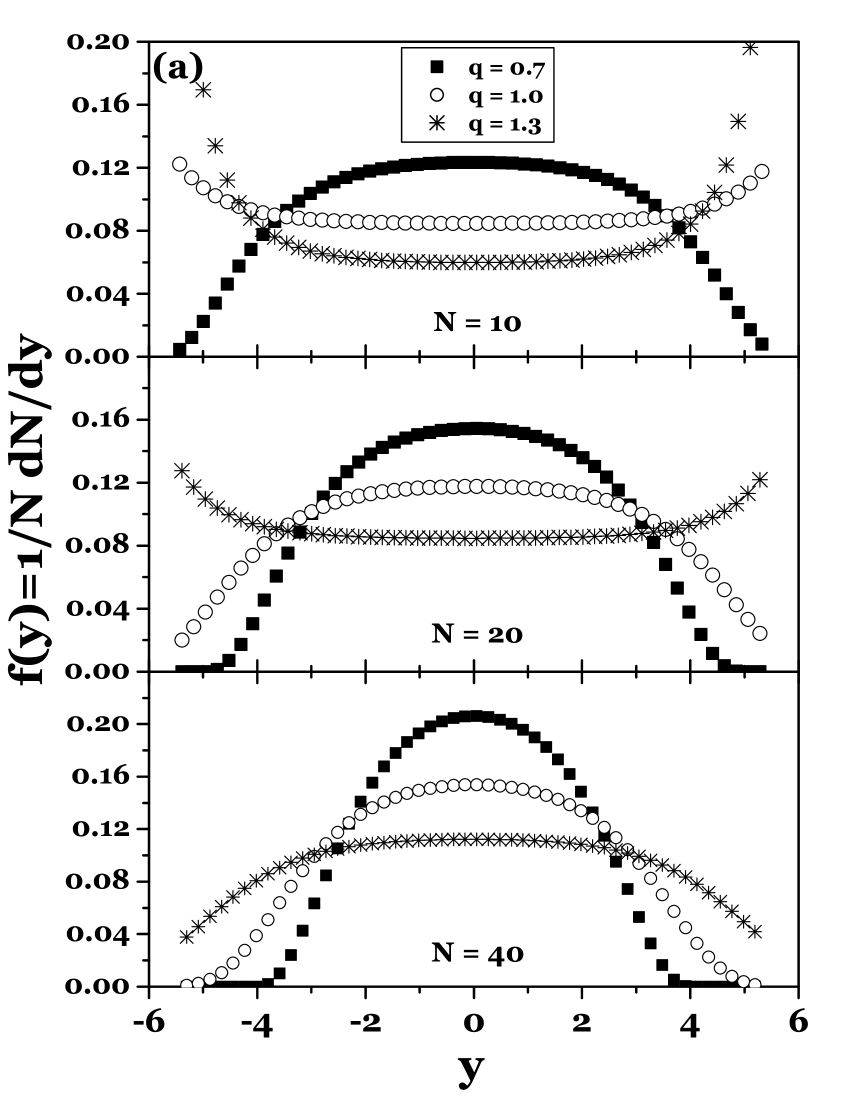
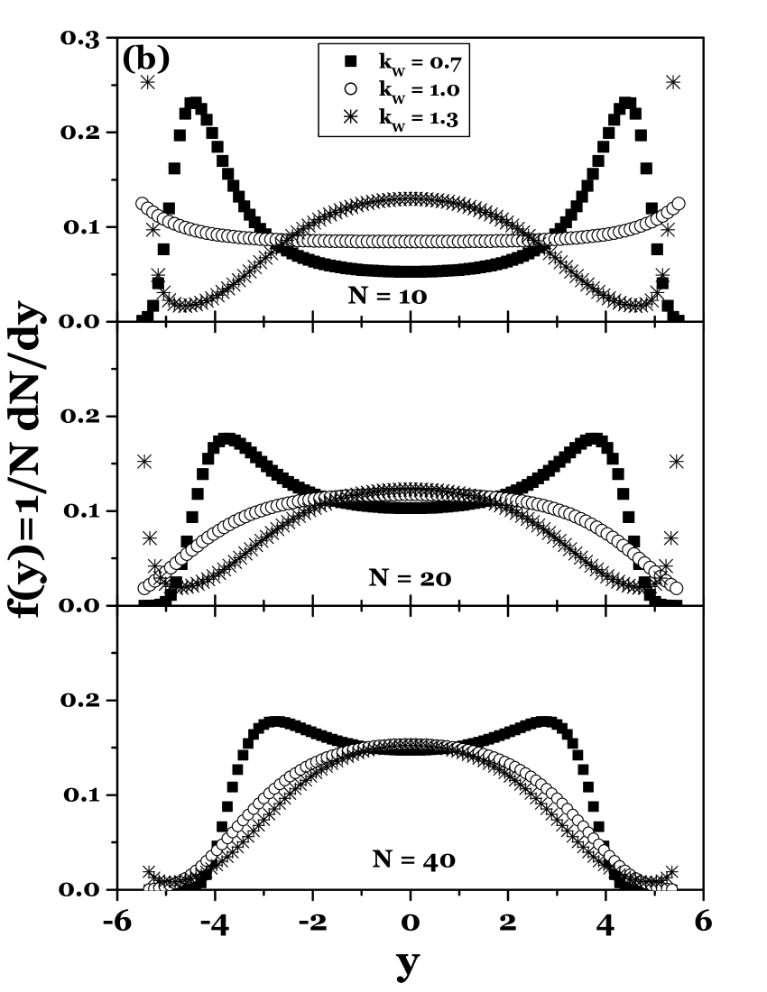
Figure 1: $(a)$ Examples of the most probable rapidity distributions as given by eq. (7) for hadronizing mass $M=100$ GeV decaying into $N$ secondaries of (transverse) mass $m_{T}=0.4$ GeV each for different values of $q$ parameter. $(b)$ The same but using eq. (4) with different values of fluctuations given by $k_{W}$ such that $W=k_{W}^{2}W_{0}$ where $W_{0}$ are the intrinsic statistical fluctuations present in the system when $\gamma=0$, i.e., where gaussian becomes pure exponential.

which confronts rapidity distributions of the Tsallis type (7) with those obtained from EGE (4) obtained for hadronization of some fixed mass $M$ into different number of secondaries. Results obtained using EGE show completely different behavior from Tsallis statistics approach clearly demonstrating that direct fluctuations in energy used in EGE (and characterized here by parameter $k_{W}$ such that $W=k_{W}^{2}W_{0}$ where $W_{0}$ are the intrinsic statistical fluctuations present in the system when $\gamma=0$) are not equivalent to fluctuations described by parameter $q$ of Tsallis’ statistics. This can be understood in the following way. In standard description of hadronization processes by means of IT in the Shannon form we always have some (mean) number of secondaries produced $\langle N\rangle$ with (mean) energy $\langle E\rangle$ each. Allowing for fluctuations of $\langle N\rangle$ results in $q$-statistics using Tsallis entropy for IT MaxEntq . In this case the mean energy per particle fluctuates from event to event. Keeping now $\langle N\rangle$ fixed but introducing distribution of energy per particle (i.e., describing energy per particle by its mean and deviation from the mean) results in EGE. Evidently single particle distributions in hadronization processes follow first or second scenario, not EGE.

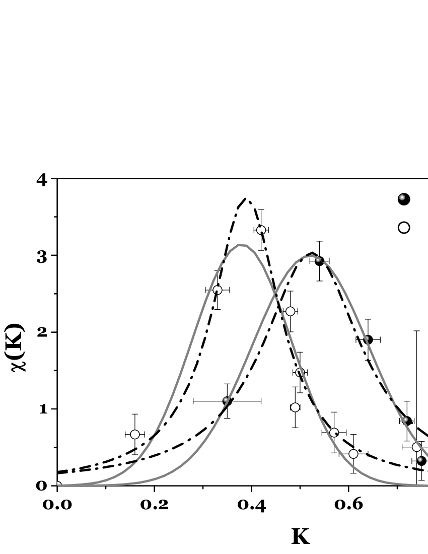
Figure 2: Inelasticity distributions $\chi(K)$ (normalized to unity) obtained in MaxEntq from analysis of multiparticle production data for $\sqrt{s}=200$ GeV and $\sqrt{s}=900$ GeV fitted by gaussian, $\chi(K)\simeq\exp\left[-(K-\langle K\rangle)^{2}/(2\sigma^{2})\right]$ (full lines), and lorentzian, $\chi(K)\simeq\sigma/[4(K-\langle K\rangle)^{2}+\sigma^{2}]$ (dash-dotted lines) formulas, respectively. The values of parameters $(<K>;\sigma)$ for gaussian case are $(0.52;0.24)$ and $(0.38;0.20)$ for $200$ GeV and $900$ GeV, respectively; for lorentzian case they are, respectively, $(0.52;0.25)$ and $(0.39;0.17)$ (see MaxEntq for more details).

On the other hand EGE turns out to be very useful when applied to other characteristic of multiparticle production, namely to inelasticity distribution, $\chi(K)$, (i.e., distribution of the fraction of the available energy, which is transformed into observed secondaries). In MaxEntq it was deduced from data for the first time for two energies: $200$ and $900$ GeV, cf. Fig. 2 (by analysing rapidity distributions of secondaries in fixed multiplicity bins). Its shape has been then fitted by gaussian and lorentzian curves but no explanation was offered for their possible origin and there was no argument at that time in favor of any of them. EGE provides arguments that most probably $\chi(K)$ should be of gaussian shape. To show this let us again follow eGe and let us suppose that the whole energy available for a given multiparticle production reaction, $E=\sqrt{s}$, is divided into two parts: one part equal to $E_{1}=K\cdot\sqrt{s}$ is going into system producing observed secondaries whereas the rest of it, $E_{2}=E-E_{1}$, is not used for this purpose and, in a sense, acts as a kind of ”heath bath” (or environment) for the first one. Both systems, the one producing particles with energy $E_{1}$ and the environment with energy $E_{2}$ can be in many possible states. Therefore

$$p_{1}(E_{1})=\frac{\Omega_{1}(E_{1})\Omega_{2}(E_{2})}{\Omega_{1+2}(E)},$$ (9)

where $\Omega$ denote the corresponding number of states. Defining entropy in the usual way as

$$S_{i}(E_{i})=\ln\Omega_{i}(E_{i}),\qquad i=1,2$$ (10)

one gets

$$p_{1}(E_{1})=\frac{1}{\Omega_{1+2}(E)}\cdot\exp\left[S_{1}(E_{1})+S_{2}(E_{2})\right].$$ (11)

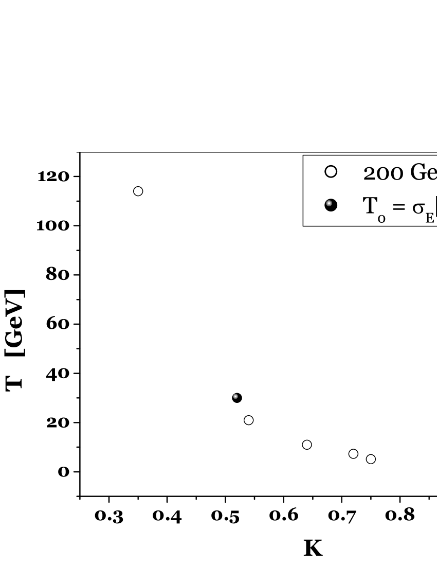
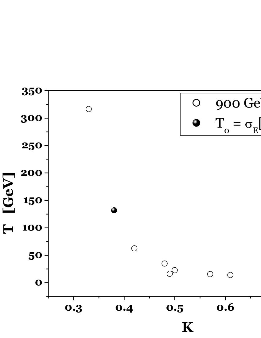
Figure 3: Inelasticity dependence of the temperature parameter as deduced in MaxEntq from multiparticle data at energies $200$ and $900$ GeV. Black circles correspond to the corresponding temperature obtained from the thermodynamical analysis performed along the EGE ideas.

Expanding now entropy around $E_{1}=U$, keeping only linear and quadratic terms and assuming that $\beta=\frac{1}{T_{0}}=\left[\frac{\partial\ln\Omega}{\partial E_{1}}\right]_{E_{1}=U}$ and $\gamma=-\left[\frac{\partial^{2}\ln\Omega}{\partial E_{1}^{2}}\right]$ are the same for both parts of the system (generalization is straightforward) one immediately obtains gaussian-like form for energy $E_{1}$ distribution,

$$p_{1}(E_{1})=\frac{1}{Z_{G}}\exp\left[-\gamma\left(E_{1}-U\right)^{2}\right],$$ (12)

which, because $E_{1}=\sqrt{s}\cdot K$ and $U=\sqrt{s}\cdot\langle K\rangle$ (where $\sqrt{s}$ is energy of reaction), translates in natural way to gaussian distribution of inelasticity, $\chi(K)$, as the most probably form with $\sigma^{2}=\frac{1}{2\gamma}$. From MaxEntq one can also deduce the $K$ dependence of the temperature $T$. Notice that in our case parameter $\gamma$ can be connected with $T$ and heat capacity $C_{V}$ because $\gamma=1/(C_{V}T^{2}_{0})$. On the other hand MaxEntq provides us also with parameter $q$ for different inelasticities for both energies and we know that $C_{V}$ can be connected with the nonextensivity parameter $q$, namely $1/C_{V}=q-1$ WW . It means therefore that there is simple relation connecting the width $\sigma$ of the observed gaussian distribution (i.e., parameter $\gamma$ of EGE), the temperature $T_{0}$ and the nonextensivity parameter $q$ describing internal behavior of the selected subsystem, namely

$$T_{0}=\sqrt{2(q-1)}\sigma_{E}\qquad{\rm where}\qquad\sigma_{E}=\sigma\cdot\sqrt{s}.$$ (13)

As can be seen in Fig. 3, $T_{0}$ deduced in such way agrees very well with the $(T,K)$ dependence deduced from analysis of rapidity distributions in fixed multiplicity bins MaxEntq .

4 Conclusions

We would like to conclude with the following remarks:

• EGE works only for the whole system, not for a single particle. This is going to be emitted according to its own distribution, in particular Boltzmann-Gibbs or Tsallis, notwithstanding what the energy $E_{1}$ is and how it is distributed. For a moment we cannot offer any convincing explanation why it is so.

• EGE is not the same (i.e., it does not describes the same kind of fluctuations) as $q$-statistics. It means that even if for some limiting cases both distribution can be similar this is just an artifact.

• On the other hand EGE tells us that for the system under consideration $T=T(E)$ and $E_{1}$ fluctuates. This means that for particles emitted from this system one should rather use Tsallis distributions reserving Boltzmann-Gibbs ones only to the case of $T$=const.

Let us close with remark that the lorentzian curve shown also in Fig. 2 (and fitting data at least as well as the gaussian one) could be explained as a kind of a nonextensive extension of EGE by noticing that in q-statistical approach one gets gaussian distribution for $q=1$ and lorentzian distribution for $q=2$. We shall not pursue this further here.

Acknowledgments: GW is grateful to the organizers of the NEXT2005 for their hospitality. Partial support of the Polish State Committee for Scientific Research (KBN) (grant 621/E-78/SPUB/CERN/P-03/DZ4/99(GW)) is acknowledged.

References

- (1) F. O. Durães, F. S. Navarra and G. Wilk, Braz. J. Phys. 35, 3 (2005).
- (2) Cf., for example, F. Becattini, Nucl. Phys. A 702, 336 (2002); F. Becattini and G. Passaleva, Eur. Phys. J. C 23, 551 (2002); W. Broniowski and W. Florkowski, Phys. Rev. Lett. 87, 272302 (2001) and Acta Phys. Polon. B 35, 779 (2004) and references therein.
- (3) G. Wilk and Z. Włodarczyk, Phys. Rev. D 43, 794 (1991).
- (4) F. S. Navarra, O. V. Utyuzh, G. Wilk and Z. Włodarczyk, Phys. Rev. D 67, 114002 (2003).
- (5) F. S. Navarra, O. V. Utyuzh, G. Wilk and Z. Włodarczyk, Physica A 340, 467 (2004).
- (6) F. S. Navarra, O. V. Utyuzh, G. Wilk and Z. Włodarczyk, Physica A 344, 568 (2004) and Nukleonika 49 (Supplement 2), s19 (2004), see also O. V. Utyuzh, G. Wilk and Z. Włodarczyk, Multiparticle production processes from the Information Theory point of view, hep-ph/0503048, to be published in Acta Phys. Hung. (HIP) (2005).
- (7) G. Wilk and Z. Wlodarczyk, Phys. Rev. Lett. 84, 2770 (2000); Chaos, Solitons and Fractals 13/3, (2001) 581; Physica A 305, 227 (2002). Cf. also: C. Beck and E. G. D.Cohen, Physica A 322, 267 (2003) and T. S. Biró and A. Jakovác, Phys. Rev. Lett. 94, 132302 (2005).
- (8) A. Giovannini and L. Van Hove, Z. Phys. C 30, 381(1986) 381; see also: P. Carruthers and C. S. Shih, Int. J. Mod. Phys. A 2, 1447 (1986).
- (9) C. Tsallis, Physica A 340, 1 (2004) and Physica A 344, 718 (2004) and references therein.
- (10) R.S.Johal, A.Planes and E.Vives, Phys. Rev. E68 (2003) 056113.
- (11) M. P. Almeida, Physica A 300, 424 (2001).
- (12) M. S. S. Challa and J. H. Hetherington, Phys. Rev. Lett. 60, 77 (1988).