PSI-PR-05-09
ZU-TH 18/05
DFTT 30/05

Electroweak corrections to ${\mathrm{W}}\gamma$ and ${\mathrm{Z}}\gamma$ production
at the LHC

E. Accomando¹, A. Denner², C. Meier^2,3

¹ Dipartimento di Fisica Teorica, Università di Torino,
Via P. Giuria 1, 10125 Torino, Italy

² Paul Scherrer Institut, Würenlingen und Villigen
CH-5232 Villigen PSI, Switzerland

³ Institute for Theoretical Physics
University of Zürich, CH-8057 Zürich, Switzerland

Abstract:

We have calculated the electroweak ${\cal O}$($\alpha$) corrections to the processes ${\mathrm{p}}{\mathrm{p}}\rightarrow{\mathrm{Z}}\gamma+X\rightarrow\nu_{l}\bar{\nu}_{l}\gamma+X$, ${\mathrm{p}}{\mathrm{p}}\rightarrow{\mathrm{Z}}\gamma+X\rightarrow l\bar{l}\gamma+X$, and ${\mathrm{p}}{\mathrm{p}}\rightarrow{\mathrm{W}}\gamma+X\rightarrow\nu_{l}\bar{l}\gamma+X$ at the LHC, with $l={\mathrm{e}},\mu$ and $\nu_{l}=\nu_{{\mathrm{e}}},\nu_{\mu},\nu_{\tau}$. The virtual corrections are evaluated in leading-pole approximation, whereas the real corrections are taken into account exactly. These corrections are implemented into a Monte Carlo generator which includes both phase-space slicing and subtraction to deal with soft and collinear singularities. We present numerical results for total cross sections as well as for experimentally interesting distributions. Applying typical LHC cuts, the electroweak corrections are of the order of $-5\%$ for the total cross sections and exceed $-20\%$ for observables dominated by high centre-of-mass energies of the partonic processes.

September 2005

1 Introduction

One of the primary goals of future colliders is to look for effects of theories beyond the Standard Model (SM). In general, there are two possibilities for new physics. Either the novel phenomena manifest themselves at energy scales probed directly at forthcoming experiments or at much larger scales. In the first case one could admire a spectacular scenario, characterized by the appearance of many new particles or resonances. In the latter case, the situation appears less favourable, but new-physics effects could still be detected in an indirect way. They can, for instance, influence physical observables at low energy by modifying the structure of the gauge-boson self-interactions. Such modifications can be parametrized in terms of anomalous couplings in the Yang–Mills vertices. While the gauge-boson couplings to the fermions have been measured at LEP2 and Tevatron to an accuracy of $0.1$–$1\%$ [1], triple and quartic gauge-boson couplings have been determined to much lower accuracy [1, 2]. Hence, the possibility of the existence of anomalous couplings in the electroweak gauge sector cannot be ruled out yet.

Vector-boson pair-production processes turn out to be especially suited for testing the non-Abelian structure of the SM. In the last decade, their potential has been extensively exploited at LEP2 and Tevatron. For these processes, the effect of anomalous couplings is expected to rise strongly with increasing invariant mass of the gauge-boson pair, since non-standard terms lead in general to unitarity violation for longitudinal gauge bosons. At future colliders, it will thus be worthwhile to analyse the large di-boson invariant-mass region. Another interesting property of the vector-boson pair-production processes is the so-called radiation zero, which characterizes the SM partonic amplitudes of ${\mathrm{W}}\gamma$ and ${\mathrm{W}}{\mathrm{Z}}$ production. Owing to gauge cancellations, for a given value of the scattering angle in the di-boson rest frame, the amplitude for ${\mathrm{W}}\gamma$ production vanishes exactly and the one for ${\mathrm{W}}{\mathrm{Z}}$ approximately. For hadronic processes, the resulting effect is the appearance of a dip in the angular distributions (see e.g. Ref. [3] and references therein). Any deviation from the SM gauge structure tends to modify this peculiar signature, thus providing a clean possibility to look for new physics. Present experiments are not sensitive enough to see the dip [4, 5], but the LHC offers the possibility to observe it for the first time.

Finally, the production of vector-boson pairs constitutes an important background in the search for new particles. For example, $\gamma{\mathrm{Z}}$ production with the ${\mathrm{Z}}$ boson decaying into a pair of neutrinos gives rise to a photon-plus-missing-energy signature. The same signal is expected for processes where the photon is produced in association with one or more heavy particles which escape the detector, either because they are weakly interacting or because they dissociate into invisible decay products. Many extensions of the SM predict the existence of such processes. For example, the ADD model [6] and related models [7, 8], where gravity becomes strong at $\,\mathrm{TeV}$ energies, predict the possibility to observe the production of a photon along with a graviton. Higher-dimensional gravitons appear as massive spin-2 neutral particles, which cannot be directly observed in a detector. Hence, graviton radiation leads to a missing-energy signature where a photon is produced with no observable particle balancing its transverse momentum. Independently of the considered new-physics model, the production of such heavy invisible particles can be inferred from the missing transverse energy distribution, which would exhibit an excess of events at high values as compared to the SM. Existing experimental searches for such an effect are, for instance, presented in Refs. [9, 10].

Owing to their limited energy and luminosity, LEP2 and Tevatron only provide weak constraints on anomalous couplings and production rates for new particles [1, 11, 12, 13]. At the LHC, the experimental collaborations will collect hundred thousands of events coming from vector-boson pair production [14]. To match the precision of the LHC experiments, the cross sections for vector-boson pair-production processes have to be calculated beyond leading order. The next-to-leading-order (NLO) QCD corrections for on-shell ${\mathrm{W}}$ and ${\mathrm{Z}}$ bosons were calculated in Refs. [15, 16] and extended to include leptonic decays in the narrow-width approximation and anomalous couplings in Refs. [17, 18, 19]. After the full NLO amplitudes including leptonic decays had become available [20], Monte Carlo programs incorporating these amplitudes have been presented for ${\mathrm{W}}\gamma$ and ${\mathrm{Z}}\gamma$ production in Ref. [21] and for ${\mathrm{W}}{\mathrm{W}}$, ${\mathrm{W}}{\mathrm{Z}}$, and ${\mathrm{Z}}{\mathrm{Z}}$ production in Refs. [22, 23]. As a general feature, the QCD corrections modify the leading-order di-boson cross sections at the LHC by a positive amount of several tens of per cent, and have thus a considerable impact on the measurement of gauge-boson couplings. At this point, the question arises if the electroweak corrections to vector-boson pair-production processes at the LHC lead to similarly sizable effects. In the above-mentioned calculations typically only universal electroweak corrections were taken into account such as the running of $\alpha$ or corrections associated with the $\rho$-parameter. This approach was based on the idea that nonuniversal electroweak corrections only contribute significantly in the high-energy domain, where the statistics at the LHC will be too low to extract any physics from the experimental data.

However, this is in general not the case in the high-energy region, which is of considerable experimental interest since as discussed above the effects of the anomalous couplings and the effects of the production of so far unknown heavy particles are most pronounced there. In fact, at high energies the electroweak corrections are enhanced by so-called electroweak Sudakov logarithms, i.e. double logarithms of the process energy over the vector-boson mass [24, 25, 26, 27, 28]. They can reach several tens of per cent and have to be taken into account to make sure that an experimentally observed deviation from the QCD-corrected SM predictions due to electroweak effects is not misinterpreted as a signal for physics beyond the SM. The importance of the electroweak corrections to gauge-boson pair-production processes at the LHC has been confirmed by several calculations [29, 30, 31], which all point to a negative contribution of some ten per cent, which well exceeds the statistical errors. Whereas the logarithmic electroweak corrections to ${\mathrm{W}}{\mathrm{W}}$, ${\mathrm{W}}{\mathrm{Z}}$, ${\mathrm{Z}}{\mathrm{Z}}$ production in the high-energy limit have been calculated including the corrections to the decay process as well as the complete real corrections [31], for ${\mathrm{W}}\gamma$ production only the logarithmic electroweak corrections to the production subprocess are available [29]. The electroweak corrections to ${\mathrm{Z}}\gamma$ production have so far only been determined for an on-shell ${\mathrm{Z}}$ boson, i.e. without taking into account decay effects [30]. Furthermore, the real corrections for the latter two processes have been included only in the soft and collinear limits or not at all. The goal of our work is therefore the calculation of the virtual and real electroweak corrections to the cross sections and distributions for the purely leptonic channels ${\mathrm{p}}{\mathrm{p}}\to V\gamma+X\to l_{1}\bar{l}_{2}\gamma+X$, where $V={\mathrm{W}},{\mathrm{Z}}$. Final states containing quarks are not discussed in this work.

This paper is organized as follows: The strategy of our calculation is described in Section 2. In Section 3 we give the setup for the numerical evaluation. Numerical results are presented in Section 4, and Section 5 contains our summary. Finally, some explicit analytical results are listed in the appendices.

2 Strategy of the calculation

We consider the production of a photon along with a massive gauge boson in proton–proton collisions, where the gauge boson decays leptonically. The generic process reads

$${\mathrm{p}}+{\mathrm{p}}\to V+\gamma+X\to l_{3}+\bar{l}_{4}+\gamma+X,$$ (2.1)

where ${\mathrm{p}}$ denotes the incoming protons, $V$ indicates a ${\mathrm{W}}$ or ${\mathrm{Z}}$ boson, $\gamma$ the outgoing photon, $l_{3}$ the outgoing lepton, $\bar{l}_{4}$ the outgoing anti-lepton, and $X$ the remnants of the protons.

In the parton model, the corresponding cross section is obtained as a convolution of the distributions $\Phi_{q_{1}|{\mathrm{p}}}$ and $\Phi_{\bar{q}_{2}|{\mathrm{p}}}$ of the partons $q_{1}$ and $\bar{q}_{2}$ in the incoming protons with the partonic cross sections $\sigma_{q_{1}\bar{q}_{2}}$, averaged over spins and colours of the partons,

$$\sigma_{{\rm{\mathrm{p}}{\mathrm{p}}}}(S)=\sum_{q_{1},q_{2}}\int_{0}^{1}{\rm d}x_{1}\int_{0}^{1}{\rm d}x_{2}\,\Phi_{q_{1}|{\mathrm{p}}}(x_{1})\Phi_{\bar{q}_{2}|{\mathrm{p}}}(x_{2})\sigma_{q_{1}\bar{q}_{2}}(\hat{s}).$$ (2.2)

The sum $\sum_{q_{1},q_{2}}$ runs over all partonic initial states which are allowed by charge conservation. In practice we include the quarks and antiquarks $q_{i}={\mathrm{u}},\bar{\mathrm{u}},{\mathrm{d}},\bar{\mathrm{d}},{\mathrm{s}},\bar{\mathrm{s}},{\mathrm{c}},\bar{\mathrm{c}}$. The integration variables $x_{i},i=1,2$ correspond to the partonic energy fractions. Moreover, the quantities $S$ and $\hat{s}=x_{1}x_{2}S$ are the squared CM energies of the hadronic process and the partonic subprocesses, respectively.

For the partonic processes we adopt the generic notation

$$q_{1}(p_{1},\sigma_{1})+\bar{q}_{2}(p_{2},\sigma_{2})\rightarrow V(p_{3}+p_{4})+\gamma(p_{5},\lambda_{5})\\ \rightarrow l_{3}(p_{3},\sigma_{3})+\bar{l}_{4}(p_{4},\sigma_{4})+\gamma(p_{5},\lambda_{5}),$$ (2.3)

where the arguments label the momenta and helicities $\sigma_{i}=\pm 1/2$, $i=1,\ldots,4$ and $\lambda_{5}=\pm 1$ of the corresponding particles. In the following, the masses of the external fermions are denoted by $m_{i}$, $i=1,\ldots,4$. Since we treat all external fermions as massless these appear only as regulators of mass singularities. The charges of the fermions are denoted by $Q_{i}$, those of the anti-fermions by $-Q_{i}$.

The lowest-order partonic cross sections are calculated using the complete matrix elements for the process

$$q_{1}(p_{1},\sigma_{1})+\bar{q}_{2}(p_{2},\sigma_{2})\rightarrow l_{3}(p_{3},\sigma_{3})+\bar{l}_{4}(p_{4},\sigma_{4})+\gamma(p_{5},\lambda_{5}).$$ (2.4)

This means that we include the full set of Feynman diagrams, in this way accounting for all irreducible background coming from non-resonant contributions. Analytic results are given in App. A.1.

The electroweak radiative corrections to (2.4) consist of virtual corrections, resulting from loop diagrams, as well as of real corrections, originating from the process

$$q_{1}(p_{1},\sigma_{1})+\bar{q}_{2}(p_{2},\sigma_{2})\to l_{3}(p_{3},\sigma_{3})+\bar{l}_{4}(p_{4},\sigma_{4})+\gamma(p_{5},\lambda_{5})+\gamma(p_{6},\lambda_{6})$$ (2.5)

with an additional photon with momentum $p_{6}$ and helicity $\lambda_{6}=\pm 1$. Virtual and real corrections have to be combined properly in order to ensure the cancellations of soft and collinear singularities (cf. Section 2.2). The helicity matrix elements for the process (2.5) are listed in App. A.3. For the calculation of the radiative corrections we follow the approach used for the process ${\mathrm{e^{+}}}{\mathrm{e^{-}}}\to{\mathrm{W^{+}}}{\mathrm{W^{-}}}\to 4f$ in Ref. [32]: The virtual corrections are calculated in the Leading-Pole Approximation (LPA), i.e. we take only those terms into account that are enhanced by a resonant massive gauge-boson propagator (cf. Section 2.3), whereas the real corrections are calculated from the full matrix elements for the processes (2.5).

2.1 Absorption of initial-state mass singularities in parton distribution functions

At next-to-leading order in electroweak perturbation theory, the partonic cross sections generally contain universal, initial-state collinear singularities. The latter can be absorbed in the Parton Distribution Functions (PDFs). To this end, one has to fix a factorization scheme, and we choose the $\overline{\rm MS}$ scheme, which defines the connection between the lowest-order PDFs in (2.2) and the experimentally determined PDFs as [33, 34]

$$\Phi_{q_{i}|{\mathrm{p}}}(x_{i})=\overline{\Phi}^{\overline{\rm MS}}_{q_{i}|{\mathrm{p}}}(x_{i},Q^{2})\\ -\frac{\alpha}{2\pi}Q_{i}^{2}\int_{x_{i}}^{1}\frac{{\rm d}z}{z}\;\overline{\Phi}^{\overline{\rm MS}}_{q_{i}|{\mathrm{p}}}\left(\frac{x_{i}}{z},Q^{2}\right)\left[\frac{1+z^{2}}{1-z}\left(\ln\left(\frac{Q^{2}}{m_{i}^{2}}\right)-2\ln(1-z)-1\right)\right]_{+}.$$ (2.6)

Here, we used the $(+)$-prescription

$$\int_{a}^{1}{\rm d}x\left[f(x)\right]_{+}g(x)=\int_{a}^{1}{\rm d}xf(x)[g(x)-g(1)]-g(1)\int_{0}^{a}{\rm d}xf(x),$$ (2.7)

and the quantity $Q$ denotes the electromagnetic factorization scale, which should be set equal to the typical energy scale of the considered process. Inserting the $\overline{\rm MS}$ definition (2.6) into the hadronic cross section (2.2) allows to write the latter as a convolution of the experimentally defined PDFs with the subtracted partonic cross section

$$\sigma_{{\rm{\mathrm{p}}{\mathrm{p}}}}(S,Q^{2})=\sum_{q_{1},q_{2}}\int_{0}^{1}{\rm d}x_{1}\int_{0}^{1}{\rm d}x_{2}\,\overline{\Phi}^{\overline{\rm MS}}_{q_{1}|{\mathrm{p}}}(x_{1},Q^{2})\overline{\Phi}^{\overline{\rm MS}}_{\bar{q}_{2}|{\mathrm{p}}}(x_{2},Q^{2})\sigma^{\overline{\rm MS}}_{q_{1}\bar{q}_{2}}(\hat{s},Q^{2}),$$ (2.8)

where

$$\sigma^{\overline{\rm MS}}_{q_{1}\bar{q}_{2}}(\hat{s},Q^{2})=\sigma_{q_{1}\bar{q}_{2}}(\hat{s})-\sigma^{\overline{\rm MS}}_{q_{1}\bar{q}_{2},{\rm sing}}(\hat{s},Q^{2})+{\cal O}(\alpha^{2})$$ (2.9)

and

$$\sigma^{\overline{\rm MS}}_{q_{1}\bar{q}_{2},{\rm sing}}(\hat{s},Q^{2})=\frac{\alpha}{4\pi\hat{s}}\sum_{i=1,2}Q_{i}^{2}\int_{0}^{1}{\rm d}z\int{\rm d}\Phi_{i}(z)\mathop{\left|{\cal M}^{(0)}_{q_{1}\bar{q}_{2}}(\Phi_{i}(z))\right|^{2}}\\ \times\frac{1}{z}\left[\frac{1+z^{2}}{1-z}\left(\ln\left(\frac{Q^{2}}{m_{i}^{2}}\right)-2\ln(1-z)-1\right)\right]_{+}.$$ (2.10)

Here ${\cal M}^{(0)}_{q_{1}\bar{q}_{2}}$ denotes the lowest-order matrix element, and $\Phi_{i}(z)$ represents the partonic phase-space where the incoming particle $i$ has momentum $zp_{i}$. After the subtraction, the resulting cross section is free of collinear and soft singularities.

A fully consistent inclusion of the electroweak corrections into the calculation of the hadronic cross sections requires the use of PDFs in which both photonic initial states and QED ${\cal{O}}(\alpha)$ corrections are taken into account. A first global analysis of parton distributions incorporating QED contributions has been performed recently in Ref. [35]. It turns out that the photon PDFs are quite small [35], and the QED corrections change the PDFs of the quarks by less than 1% [36, 37]. These effects are below the typical uncertainty of hadronic processes and below the envisaged accuracy of our analysis. Accordingly, we restrict our calculation to initial states containing quarks and use only QCD-corrected PDFs in (2.8). We nevertheless investigated the dependence of our results on the electromagnetic factorization scale $Q$ entering in (2.10), keeping the QCD factorization scale Q that enters $\overline{\Phi}^{\overline{\rm MS}}_{q_{i}|{\mathrm{p}}}(x_{i},Q^{2})$ in (2.8) fixed. For $\gamma{\mathrm{Z}}$ production, a variation of $Q$ by a factor 10 resulted in a change of the total cross section by less than 0.3%, of the $\gamma{\mathrm{Z}}$ invariant-mass distribution at large invariant mass by less than 0.5%, and of the transverse momentum distribution of the photon at large transverse momenta by less than 1%.

2.2 Treatment of soft and collinear photon emission

In first-order electroweak perturbation theory, the subtracted partonic cross section receives contributions from the lowest order, the virtual corrections, the real corrections, as well as of the term (2.10) arising from the factorization of the initial-state collinear singularities:

$$\sigma_{q_{1}\bar{q}_{2}}^{\overline{\rm MS}}(\hat{s},Q^{2})=\sigma_{q_{1}\bar{q}_{2}}^{(0)}(\hat{s})+\sigma_{q_{1}\bar{q}_{2}}^{{\rm virt}}(\hat{s})+\sigma_{q_{1}\bar{q}_{2}}^{{\rm real}}(\hat{s})-\sigma^{\overline{\rm MS}}_{q_{1}\bar{q}_{2},{\rm sing}}(\hat{s},Q^{2}).$$ (2.11)

In general, virtual and real corrections contain soft as well as collinear singularities, which we regularize by introducing an infinitesimal photon mass $m_{\gamma}$ as well as small mass parameters $m_{i}$ for the external fermions. These logarithmic singularities cancel when adding real and virtual corrections, except for the collinear logarithms arising from the initial state, which are absorbed in the PDFs as described in Section 2.1. Thus, all soft and collinear singularities cancel in (2.11), leaving the subtracted cross section free of any mass regulators.

However, this cancellation requires a careful treatment of soft and collinear singularities. In our work, we adopt the approach to divide the virtual and real corrections into finite and singular parts, and to cancel the dependence on the mass regulators by adding the singular parts analytically. To extract the singular parts from the real corrections, we employ two independent methods, the phase-space-slicing technique and the dipole subtraction method. In the following we give explicit expressions for our treatment of infrared, i.e. soft and collinear, singularities.

2.2.1 Finite virtual corrections

First, we define the finite virtual corrections by

$$\sigma_{q_{1}\bar{q}_{2},{\rm finite}}^{{\rm virt}}(\hat{s}) = \frac{1}{2\hat{s}}\int{\rm d}\Phi_{0}\,\Bigl{(}2\mathop{\mathrm{Re}}\nolimits\left[{\cal M}_{q_{1}\bar{q}_{2}}^{(0)}(\Phi_{0})\left(\delta{\cal M}_{q_{1}\bar{q}_{2}}^{{\rm virt}}(\Phi_{0})\right)^{\star}\right]$$ (2.12)

$$\qquad{}-2\mathop{\mathrm{Re}}\nolimits\left[{\cal M}_{q_{1}\bar{q}_{2}}^{(0)}(\Phi_{0})\left(\delta{\cal M}_{q_{1}\bar{q}_{2},\mathrm{sing}}^{{\rm virt}}(\Phi_{0})\right)^{\star}\right]\Bigr{)},$$

where ${\cal M}_{q_{1}\bar{q}_{2}}^{(0)}$ and $\delta{\cal M}_{q_{1}\bar{q}_{2}}^{{\rm virt}}$ denote the matrix elements of the Born process and the corresponding electroweak virtual corrections, respectively, whereas $\Phi_{0}$ is the phase-space for the Born process (2.4). The subtracted singular parts are given by [32, 38]

$$2\mathop{\mathrm{Re}}\nolimits\left[{\cal M}_{q_{1}\bar{q}_{2}}^{(0)}(\Phi_{0})\left(\delta{\cal M}_{q_{1}\bar{q}_{2},\mathrm{sing}}^{{\rm virt}}(\Phi_{0})\right)^{\star}\right]=\frac{\alpha}{2\pi}\sum_{i,j=1\atop i\neq j}^{n}\tau_{i}\tau_{j}Q_{i}Q_{j}\mathop{\left|{\cal M}_{q_{1}\bar{q}_{2}}^{(0)}(\Phi_{0})\right|^{2}}({\cal L}(s_{ij},m_{i}^{2})+C_{ij}),$$ (2.13)

where $n$ is the number of external particles of the lowest-order process, $s_{ij}=(p_{i}+p_{j})^{2}$, and $\tau_{i}=1$ for incoming particles and outgoing anti-particles, whereas $\tau_{i}=-1$ for outgoing particles and incoming anti-particles. The singularities are contained in

$${\cal L}(s_{ij},m_{i}^{2})=\ln\left(\frac{m_{\gamma}^{2}}{s_{ij}}\right)\left(1+\ln\left(\frac{m_{i}^{2}}{s_{ij}}\right)\right)-\frac{1}{2}\ln^{2}\left(\frac{m_{i}^{2}}{s_{ij}}\right)+\frac{1}{2}\ln\left(\frac{m_{i}^{2}}{s_{ij}}\right),$$ (2.14)

while the finite parts $C_{ij}$ are added for later convenience and distinguish between incoming, $i,j=1,2$, and outgoing particles, $i,j>2$,

$$C_{ij}=\left\{\begin{array}[]{l l}-\frac{\pi^{2}}{3}+\frac{3}{2},&i,j>2,\quad i\neq j,\\[4.30554pt] \phantom{-}\frac{\pi^{2}}{6}-1,&i=1,2,\quad j>2,\\[4.30554pt] -\frac{\pi^{2}}{2}+\frac{3}{2},&i>2,\quad j=1,2,\\[4.30554pt] -\frac{\pi^{2}}{3}+2,&i=1,2,\quad j=1,2,\quad i\neq j.\\[4.30554pt] \end{array}\right.$$ (2.15)

2.2.2 Phase-space slicing

In short, the idea of the phase-space-slicing technique is to define the finite real corrections by restricting the phase-space integration to the region where the squared amplitude of the bremsstrahlung process is finite. To this end, a technical cut $\delta_{\mathrm{s}}$ on the energy $E$ of the bremsstrahlung particle is introduced, as well as a technical cut $\delta_{\mathrm{c}}$ on the angles $\vartheta_{i}$ of the bremsstrahlung particles with respect to all potential emitters. The finite real corrections are then given by

$$\sigma^{{\rm real,sli}}_{q_{1}\bar{q}_{2},{\rm finite}}(\hat{s})=\frac{1}{2\hat{s}}\int_{\parbox{54.06006pt}{\tiny$E>\delta_{\mathrm{s}}\sqrt{\hat{s}}/2$\\ $\cos\vartheta_{i}<1-\delta_{\mathrm{c}}$}}{\rm d}\Phi_{{\rm real}}\mathop{\left|{\cal M}^{{\rm real}}_{q_{1}\bar{q}_{2}}(\Phi_{{\rm real}})\right|^{2}},$$ (2.16)

where $\Phi_{{\rm real}}$ and ${\cal M}^{{\rm real}}$ denote the phase-space and the matrix element of the bremsstrahlung process (2.5).

In the remaining singular parts of the real corrections, the momentum of the bremsstrahlung particle is integrated out, up to a remaining convolution over the momentum fraction $z$ of the initial state particle after bremsstrahlung emission. Here the soft and collinear singularities are again regularized by an infinitesimal photon mass $m_{\gamma}$ and by small mass parameters $m_{i}$ for the external fermions. The resulting expressions [32, 33] can be divided into a part arising from initial-state radiation and a part arising from final-state radiation. Adding them to the term (2.10) originating from the $\overline{\rm MS}$ definition of the PDFs and to the singular parts (2.12) of the virtual corrections, all infrared singularities cancel and one obtains a finite contribution

$$\sigma_{q_{1}\bar{q}_{2},{\mathrm{sing}}}^{{\rm virt+real,sli}}(\hat{s},Q^{2})=\sigma_{q_{1}\bar{q}_{2},{\rm sing}}^{{\rm virt}}(\hat{s})+\sigma^{{\rm real,sli}}_{q_{1}\bar{q}_{2},{\rm sing}}(\hat{s})-\sigma^{\rm\overline{\rm MS}}_{q_{1}\bar{q}_{2},{\rm sing}}(\hat{s},Q^{2})\\ =\frac{1}{2\hat{s}}\int{\rm d}\Phi_{0}\left(\mathop{\left|{\cal M}^{{\rm v+r,init}}_{q_{1}\bar{q}_{2},{\mathrm{sing}}}(\Phi_{0})\right|^{2}}+\mathop{\left|{\cal M}^{{\rm v+r,final}}_{q_{1}\bar{q}_{2},{\mathrm{sing}}}(\Phi_{0})\right|^{2}}\right)\\ +\frac{1}{2\hat{s}}\sum_{i=1}^{2}\int\frac{{\rm d}z}{z}\int{\rm d}\Phi_{i}(z)\mathop{\left|{\cal M}^{{\rm v+r,init,z}}_{q_{1}\bar{q}_{2},{\mathrm{sing}}}(\Phi_{i}(z))\right|^{2}},$$ (2.17)

where

$$\mathop{\left|{\cal M}^{{\rm v+r,init}}_{q_{1}\bar{q}_{2},{\mathrm{sing}}}(\Phi_{0})\right|^{2}}=\frac{\alpha}{2\pi}\sum_{i=1}^{2}\sum_{{j=1\atop j\neq i}}^{n}Q_{i}\tau_{i}Q_{j}\tau_{j}\mathop{\left|{\cal M}^{(0)}_{q_{1}\bar{q}_{2}}(\Phi_{0})\right|^{2}}\\ \times\left[\frac{\pi^{2}}{3}-2+C_{ij}+{\rm Li}_{2}\left(1-\frac{4E_{i}E_{j}}{s_{ij}}\right)\right.\\ \left.+\ln\left(\frac{\hat{s}}{s_{ij}}\frac{\delta_{\mathrm{c}}}{2}\right)\left(\frac{3}{2}+\ln\delta_{\mathrm{s}}^{2}\right)+\frac{1}{2}\ln^{2}\left(\frac{\hat{s}}{s_{ij}}\right)\right],$$ (2.18)

$$\mathop{\left|{\cal M}^{{\rm v+r,final}}_{q_{1}\bar{q}_{2},{\mathrm{sing}}}(\Phi_{0})\right|^{2}}=\frac{\alpha}{2\pi}\sum_{i=3}^{n}\sum_{{j=1\atop j\neq i}}^{n}Q_{i}\tau_{i}Q_{j}\tau_{j}\mathop{\left|{\cal M}^{(0)}_{q_{1}\bar{q}_{2}}(\Phi_{0})\right|^{2}}\\ \times\left[\pi^{2}-\frac{9}{2}+C_{ij}+{\rm Li}_{2}\left(1-\frac{4E_{i}E_{j}}{s_{ij}}\right)\right.\\ \left.+\ln\left(\frac{4E_{i}^{2}}{s_{ij}}\frac{\delta_{\mathrm{c}}}{2}\right)\left(\frac{3}{2}+\ln\left(\frac{\delta_{\mathrm{s}}^{2}\hat{s}}{4E_{i}^{2}}\right)\right)+\frac{1}{2}\ln^{2}\left(\frac{4E_{i}^{2}}{s_{ij}}\right)\right],$$ (2.19)

$$\mathop{\left|{\cal M}^{{\rm v+r,init,z}}_{q_{1}\bar{q}_{2},{\mathrm{sing}}}(\Phi_{i}(z))\right|^{2}}=-\frac{\alpha}{2\pi}\sum_{{j=1\atop j\neq i}}^{n}Q_{i}\tau_{i}Q_{j}\tau_{j}\mathop{\left|{\cal M}^{(0)}_{q_{1}\bar{q}_{2}}(\Phi_{i}(z))\right|^{2}}\\ \times\left[\frac{1+z^{2}}{1-z}\left(\ln\left(\frac{\hat{s}}{Q^{2}}\frac{\delta_{\mathrm{c}}}{2}\right)+2\ln(1-z)+1\right)-\frac{2z}{1-z}\right]_{+},$$ (2.20)

${\rm Li}_{2}$ denotes the dilogarithm

$${\rm Li}_{2}(z)=-\int_{0}^{z}\;\frac{{\rm d}t}{t}\ln(1-t),\qquad|\mathop{\mathrm{arc}}\nolimits(1-z)|<\pi,$$ (2.21)

and $\Phi_{i}(z)$ represents the phase-space where the incoming particle $i$ has momentum $zp_{i}$.

2.2.3 Dipole subtraction method

In the dipole subtraction method, the finite real corrections are constructed by subtracting an auxiliary function from the squared bremsstrahlung amplitude before integrating over phase-space,

$$\sigma^{{\rm real,sub}}_{q_{1}\bar{q}_{2},{\rm finite}}(\hat{s})=\frac{1}{2\hat{s}}\int{\rm d}\Phi_{{\rm real}}\left(\mathop{\left|{\cal M}^{{\rm real}}_{q_{1}\bar{q}_{2}}(\Phi_{{\rm real}})\right|^{2}}-\mathop{\left|{\cal M}^{\rm sub}_{q_{1}\bar{q}_{2}}(\Phi_{{\rm real}})\right|^{2}}\right).$$ (2.22)

The subtracted terms are added again after partial analytic integration over the bremsstrahlung momentum. The subtraction function has to be chosen such that it cancels all soft and collinear singularities of the original integrand, so that the difference (2.22) can be integrated numerically without regulators for these singularities. Moreover, it has to be simple enough so that it can be integrated analytically over the singular regions of phase space. We use the process-independent dipole subtraction formalism, which was introduced for massless QCD in Refs. [39, 40, 41] and generalized to massive fermions in Ref. [38]. We follow the approach of Ref. [38] in the limit of small fermion masses.

In the dipole subtraction formalism the subtraction function is constructed from contributions that are labelled by ordered pairs $ij$ of charged fermions, so-called dipoles. The fermions $i$ and $j$ are called emitter and spectator, respectively. In the formulation of Ref. [38] the subtraction function reads

$$\mathop{\left|{\cal M}^{\rm sub}_{q_{1}\bar{q}_{2}}(\Phi_{{\rm real}})\right|^{2}}=-4\pi\alpha\sum_{n_{b}=5}^{6}\sum_{i,j=1\atop i\neq j}^{n}\tau_{i}\tau_{j}Q_{i}Q_{j}g_{ij}^{\rm sub}(p_{i},p_{j},p_{n_{b}})\mathop{\left|{\cal M}^{(0)}_{q_{1}\bar{q}_{2}}(\tilde{\Phi}^{n_{b}}_{0,ij})\right|^{2}}.$$ (2.23)

The sum over $n_{b}=5,6$ accounts for the fact that the photon appears twice in the final state of the bremsstrahlung process (2.5), such that a separate subtraction term has to be introduced for each final-state photon. Note that one of the two final-state photons has always to be visible in the detector and thus does not give rise to singularities. In what follows, we suppress the dependence of the phase-space on $n_{b}$ and denote the bremsstrahlung momentum by $k=p_{n_{b}}$. The phase-spaces $\tilde{\Phi}^{n_{b}}_{0,ij}$ in (2.23) are given by embedding prescriptions of the phase-space $\Phi^{\rm real}$ of the bremsstrahlung process in the phase-space $\Phi_{0}$ of the Born process. Both, the embedding prescription $\tilde{\Phi}_{0,ij}^{n_{b}}$ and the subtraction functions $g_{ij}^{\rm sub}$ depend on the emitter $i$ and spectator $j$ being incoming or outgoing. One therefore encounters four kinematically different cases for the subtraction functions $g_{ij}^{\rm sub}$

$$g_{ij}^{\rm sub}(p_{i},p_{j},k)=\left\{\begin{array}[]{l l}\frac{1}{(p_{i}k)(1-y_{ij})}\left[\frac{2}{1-z_{ij}(1-y_{ij})}-1-z_{ij}\right],&\quad i,j>2,\\[6.45831pt] \frac{1}{(p_{i}k)x_{ij}}\left[\frac{2}{2-x_{ij}-z_{ij}}-1-z_{ij}\right],&\quad i>2,\quad j=1,2,\\[6.45831pt] \frac{1}{(p_{i}k)x_{ji}}\left[\frac{2}{2-x_{ji}-z_{ji}}-1-x_{ji}\right],&\quad i=1,2,\quad j>2,\\[6.45831pt] \frac{1}{(p_{i}k)v_{ij}}\left[\frac{2}{1-v_{ij}}-1-v_{ij}\right],&\quad i=1,2,\quad j=1,2.\end{array}\right.$$ (2.24)

where

$$x_{ij} =\frac{p_{i}p_{j}+p_{j}k-p_{i}k}{p_{i}p_{j}+p_{j}k}, y_{ij}=\frac{p_{i}k}{p_{i}p_{j}+p_{i}k+p_{j}k},$$

$$z_{ij} =\frac{p_{i}p_{j}}{p_{i}p_{j}+p_{j}k}, v_{ij}=\frac{p_{i}p_{j}-p_{i}k-p_{j}k}{p_{i}p_{j}}.$$ (2.25)

Denoting the number of external particles by $n$, one has for the embedding prescription if both the emitter and the spectator are part of the final state

$$\tilde{p}^{\mu}_{i}=p_{i}^{\mu}+k^{\mu}-\frac{y_{ij}}{1-y_{ij}}p^{\mu}_{j},\qquad\tilde{p}^{\mu}_{j}=\frac{1}{1-y_{ij}}p^{\mu}_{j},\qquad\tilde{p}^{\mu}_{l}=p^{\mu}_{l},\\ i,j>2,\quad i\neq j,\quad l=1,\ldots,n,\quad l\neq i,j,$$ (2.26)

whereas for an initial-state emitter and a final-state spectator one gets

$$\tilde{p}^{\mu}_{i}=x_{ji}p^{\mu}_{i},\qquad\tilde{p}^{\mu}_{j}=p^{\mu}_{j}+k^{\mu}-(1-x_{ji})p^{\mu}_{i},\qquad\tilde{p}^{\mu}_{l}=p^{\mu}_{l},\\ i=1,2,\quad j>2,\quad l=1,\ldots,n,\quad l\neq i,j.$$ (2.27)

The embedding prescription for a final-state emitter and an initial-state spectator can be obtained from (2.27) by exchanging $i\leftrightarrow j$ everywhere. Finally, in case of an initial-state emitter and an initial-state spectator the embedding prescription is given by

$$\tilde{p}_{i}^{\mu}=v_{ij}p_{i},\qquad\tilde{p}_{j}=p_{j},\qquad\tilde{p}_{l}^{\mu}=\Lambda_{\;\;\nu}^{\mu}p_{l}^{\nu},\qquad i,j=1,2,\quad i\neq j,\quad l=3,\ldots,n$$ (2.28)

with the boost matrix

$$\Lambda_{\;\;\nu}^{\mu}=g_{\;\;\nu}^{\mu}-\frac{(P_{ij}+\tilde{P}_{ij})^{\mu}(P_{ij}+\tilde{P}_{ij})_{\nu}}{P_{ij}^{2}+P_{ij}\tilde{P}_{ij}}+\frac{2\tilde{P}_{ij}^{\mu}P_{ij,\nu}}{P_{ij}^{2}}.$$ (2.29)

Here, $\tilde{P}_{ij}$ represents the total initial-state momentum after the projection, $\tilde{P}_{ij}^{\mu}=\tilde{p}_{i}^{\mu}+\tilde{p}_{j}^{\mu}$, and

$$P_{ij}=p_{1}+p_{2}-k=\sum_{k=3}^{n}p_{k}.$$ (2.30)

The subtracted contribution can be integrated over the (singular) photonic degrees of freedom up to a remaining convolution over a variable $z$. In this integration the regulators $m_{\gamma}$ and $m_{i}$ must be retained, and soft and collinear singularities appear as logarithms in these mass regulators. The resulting expressions [32, 38] can again be divided into a part arising from initial-state radiation and a part arising from final-state radiation. Adding them to the term (2.10) originating from the $\overline{\rm MS}$ definition of the PDFs and to the singular parts (2.12) of the virtual corrections, the infrared singularities cancel and one finds

$$\sigma_{q_{1}\bar{q}_{2},{\mathrm{sing}}}^{{\rm virt+real,sub}}(\hat{s},Q^{2})=\sigma_{q_{1}\bar{q}_{2},{\rm sing}}^{{\rm virt}}(\hat{s})+\sigma^{{\rm real,sub}}_{q_{1}\bar{q}_{2},{\rm sing}}(\hat{s})-\sigma^{\rm\overline{\rm MS}}_{q_{1}\bar{q}_{2},{\rm sing}}(\hat{s},Q^{2})\\ =\frac{1}{2\hat{s}}\sum_{i=1}^{2}\int\frac{{\rm d}z}{z}\int{\rm d}\Phi_{i}(z)\left(\mathop{\left|{\cal M}^{{\rm v+r,init,z}}_{q_{1}\bar{q}_{2},{\mathrm{sing}}}(\Phi_{i}(z))\right|^{2}}+\mathop{\left|{\cal M}^{{\rm v+r,final,z}}_{q_{1}\bar{q}_{2},{\mathrm{sing}}}(\Phi_{i}(z))\right|^{2}}\right),$$ (2.31)

where

$$\mathop{\left|{\cal M}^{{\rm v+r,init,z}}_{q_{1}\bar{q}_{2},{\mathrm{sing}}}(\Phi_{i}(z))\right|^{2}}=-\frac{\alpha}{2\pi}\sum_{{j=1\atop j\neq i}}^{n}Q_{i}\tau_{i}Q_{j}\tau_{j}\mathop{\left|{\cal M}^{(0)}_{q_{1}\bar{q}_{2}}(\Phi_{i}(z))\right|^{2}}\\ \times\left[\frac{1+z^{2}}{1-z}\left(\ln\left(\frac{|\tilde{s}_{ij}|}{Q^{2}z}\right)+2\ln(1-z)\right)+1-z\right.\\ \left.-\delta_{j>2}\left(\frac{2}{1-z}\ln(2-z)-(1+z)\ln(1-z)\right)\right]_{+},$$ (2.32)

$$\mathop{\left|{\cal M}^{{\rm v+r,final,z}}_{q_{1}\bar{q}_{2},{\mathrm{sing}}}(\Phi_{i}(z))\right|^{2}}\\ =\frac{\alpha}{2\pi}Q_{i}\tau_{i}(\tau_{1}Q_{1}+\tau_{2}Q_{2})\mathop{\left|{\cal M}^{(0)}_{q_{1}\bar{q}_{2}}(\Phi_{i}(z))\right|^{2}}\left[\frac{1}{1-z}\left(2\ln\left(\frac{2-z}{1-z}\right)-\frac{3}{2}\right)\right]_{+},$$ (2.33)

and $\delta_{j>2}=1$ for $j>2$ and $\delta_{j>2}=0$ for $j\leq 2$. Note that the finite part (2.15) of the singular virtual corrections (2.13) has been chosen to exactly cancel the end-point parts resulting from the subtraction function (2.23) such that only $z$-dependent contributions remain in (2.32) and (2.33).

2.2.4 Master formula

Altogether, in our approach the subtracted partonic cross section, which is free of soft and collinear singularities, can be written as a sum of four different parts

$$\sigma_{q_{1}\bar{q}_{2}}^{\overline{\rm MS}}(\hat{s},Q^{2})=\sigma_{q_{1}\bar{q}_{2}}^{(0)}(\hat{s})+\sigma_{q_{1}\bar{q}_{2},{\rm finite}}^{{\rm virt}}(\hat{s})+\sigma_{q_{1}\bar{q}_{2},{\rm finite}}^{{\rm real}}(\hat{s})+\sigma_{q_{1}\bar{q}_{2},{\rm sing}}^{{\rm virt+real}}(\hat{s},Q^{2}),$$ (2.34)

where the finite virtual corrections in the second term of the right-hand side are defined by (2.12). The last two terms are given by (2.16) and (2.17), respectively, if using the phase-space-slicing technique and by (2.22) and (2.31), respectively, in case of using the subtraction method.

2.3 Treatment of finite-width effects

The processes (2.3) involve the production and decay of an unstable particle $V={\mathrm{W}},{\mathrm{Z}}$. The corresponding propagator leads to a pole in the amplitude, which has to be regularized by incorporating the finite width of the massive vector bosons. Several methods to include finite-width effects in a perturbative calculation have been discussed in the literature [42, 43, 44, 45, 46, 47, 48, 49, 50, 51, 52, 53]. The simplest approach is given by the fixed-width scheme, which corresponds to replacing the resonant propagator by one containing a constant finite width. Since the finite width results from resummation of an incomplete set of higher-order contributions, its introduction potentially violates gauge invariance. For Born amplitudes, the effects of this violation have been shown to be numerically small in the fixed-width scheme (see e.g. Refs. [45, 47, 54, 55]) by comparing the results to those obtained with other manifestly gauge-invariant prescriptions, as e.g. the complex-mass scheme [47].

In our calculation, following the approach of Ref. [32], we adopt the fixed-width scheme to evaluate the Born cross section and the real corrections. For the virtual corrections, on the other hand, we use the LPA [32, 43, 46]. In this approximation only the leading term in an expansion about the resonance pole, i.e. the residue divided by the resonant propagator, is kept. Since the residue, which is related to physical amplitudes for on-shell production and decay, and the resonant propagator are gauge-invariant, the LPA yields a gauge-invariant result. As all non-resonant contributions are neglected, the number of contributing diagrams is considerably reduced, and only loop integrals with up to four propagators appear. The error induced by using the LPA for the virtual corrections can be estimated to be of the order $\alpha\Gamma_{V}/M_{V}$, where $M_{V}$ and $\Gamma_{V}$ are the mass and the width of the vector boson $V$, respectively, and thus of the order of a few per mille. This estimate was confirmed for single W production at hadron colliders in Ref. [34] and for WW production in electron positron annihilation in Refs. [56, 57]. Thus, the LPA should be more than sufficient for the considered process, as long as the resonant diagrams dominate.

Following the approach presented in Ref. [32], the virtual corrections evaluated in LPA can be further split into factorizable and non-factorizable parts, such that the finite virtual corrections can be written as

$$\sigma_{q_{1}\bar{q}_{2},{\rm finite}}^{{\rm virt},{\rm LPA}}(\hat{s})=\frac{1}{2\hat{s}}\int{\rm d}\Phi_{0}\,2\mathop{\mathrm{Re}}\nolimits\left[{\cal M}^{(0),{\rm LPA}}_{q_{1}\bar{q}_{2}}(\Phi_{0},\Phi_{0}^{\rm osh})\right.\\ \times\left.\left(\delta{\cal M}^{{\rm virt},{\rm LPA}}_{q_{1}\bar{q}_{2},{\rm fac}}(\Phi_{0},\Phi_{0}^{\rm osh})+\delta{\cal M}_{q_{1}\bar{q}_{2},{\rm nfac}}^{{\rm virt},{\rm LPA}}(\Phi_{0},\Phi_{0}^{\rm osh})-\delta{\cal M}_{q_{1}\bar{q}_{2},{\rm sing}}^{{\rm virt},{\rm LPA}}(\Phi_{0},\Phi_{0}^{\rm osh})\right)^{\star}\right].$$ (2.35)

In (2.35), ${\cal M}^{(0),{\rm LPA}}_{q_{1}\bar{q}_{2}}(\Phi_{0},\Phi_{0}^{\rm osh})$ denotes the Born matrix element in LPA

$${\cal M}^{(0),{\rm LPA}}_{q_{1}\bar{q}_{2}}(\Phi_{0},\Phi_{0}^{\rm osh})=\frac{R^{(0)}(\Phi_{0}^{\rm osh})}{(p_{3}+p_{4})^{2}-M_{V}^{2}+{\mathrm{i}}M_{V}\Gamma_{V}},$$ (2.36)

which receives contributions from all Born diagrams containing the resonant propagator. The residue $R$ of the amplitude at the pole is evaluated using a phase-space $\Phi^{\rm osh}_{0}=\{p_{i}^{\rm osh},i=1,\ldots,5\}$ projected on the mass-shell of the decaying particle, i.e. $(p_{3}^{\rm osh}+p_{4}^{\rm osh})^{2}=M_{V}^{2}$. We specify our choice for the on-shell projection in App. B. The factorizable virtual corrections in (2.35) get contributions from all diagrams where the resonant propagator appears outside the loop, i.e. from diagrams that factorize into a production part, a decay part, and the resonant propagator. In LPA, they can be written as

$$\delta{\cal M}_{q_{1}\bar{q}_{2},{\rm fac}}^{{\rm virt},{\rm LPA}}(\Phi_{0},\Phi_{0}^{\rm osh})=\frac{R_{{\rm fac}}^{{\rm virt}}(\Phi_{0}^{\rm osh},m_{\gamma})}{(p_{3}+p_{4})^{2}-M_{V}^{2}+{\mathrm{i}}M_{V}\Gamma_{V}},$$ (2.37)

where all soft singularities are regularized by the infinitesimal photon mass parameter $m_{\gamma}$.

The non-factorizable virtual corrections receive contributions from all diagrams where a massless virtual particle, in our case a photon, connects the production and decay subprocesses or one of these subprocesses to the resonance. The infrared singularities originating from photon emission off the unstable boson $V$ are here regularized by keeping the resonant momentum off-shell wherever the on-shell limit leads to a singularity. The contribution of the diagrams where the photon couples to the resonance are already partly contained in the factorizable virtual corrections as defined above, such that this contribution has to be subtracted from the non-factorizable corrections to avoid double counting [32]. As an advantage, the non-factorizable virtual corrections can be evaluated in the Extended Soft Photon Approximation (ESPA), which corresponds to setting the loop momentum to zero wherever this does not lead to a resonance. The non-factorizable corrections

$$\delta{\cal M}_{q_{1}\bar{q}_{2},{\rm nfac}}^{{\rm virt},{\rm LPA}}(\Phi_{0},\Phi_{0}^{\rm osh})=\frac{R_{{\rm nfac}}^{{\rm virt},{\rm ESPA}}(\Phi_{0}^{\rm osh},(p_{3}+p_{4})^{2}-M_{V}^{2})}{(p_{3}+p_{4})^{2}-M_{V}^{2}+{\mathrm{i}}M_{V}\Gamma_{V}}\\ =\frac{1}{2}{\cal M}^{(0),{\rm LPA}}_{q_{1}\bar{q}_{2}}(\Phi_{0},\Phi_{0}^{\rm osh})\delta^{{\rm virt}}_{{\rm nfac}}(\Phi_{0}^{\rm osh},(p_{3}+p_{4})^{2}-M_{V}^{2}),$$ (2.38)

are then proportional to the Born matrix element in LPA. We give the analytical expression for the correction factor $\delta^{{\rm virt}}_{{\rm nfac}}$ in App. A.2.

Note that in order not to spoil the cancellation of soft and collinear singularities between the virtual corrections in LPA and the real corrections evaluated exactly, we consistently subtract in (2.35) the singular virtual corrections evaluated in LPA

$$2\mathop{\mathrm{Re}}\nolimits\left[{\cal M}^{(0),\mathrm{LPA}}_{q_{1}\bar{q}_{2}}(\Phi_{0},\Phi_{0}^{\rm osh})\left(\delta{\cal M}_{q_{1}\bar{q}_{2},{\rm sing}}^{{\rm virt,LPA}}(\Phi_{0},\Phi_{0}^{\rm osh})\right)^{\star}\right]\\ =\frac{\alpha}{2\pi}\sum_{i,j=1\atop i\neq j}^{n}\tau_{i}\tau_{j}Q_{i}Q_{j}\mathop{\left|{\cal M}_{q_{1}\bar{q}_{2}}^{(0),{\rm LPA}}(\Phi_{0},\Phi_{0}^{\rm osh})\right|^{2}}({\cal L}(s^{\rm osh}_{ij},m_{i}^{2})+C_{ij}),$$ (2.39)

but we use the exact singular virtual corrections in (2.17) and (2.31). In (2.39), $s_{ij}^{\rm osh}=(p_{i}^{\rm osh}+p_{j}^{\rm osh})^{2}$, and ${\cal L}$ and $C_{ij}$ are given by (2.14) and (2.15), respectively.

2.4 Implementation

We have implemented our strategy in a Mathematica package called Pole, which works as an extension of the computer-algebra packages FeynArts3 [58] and FormCalc3.1 [59]. To be explicit, Pole extends these packages by the following features:

• amplitude generation for initial-state hadrons,

• amplitude generation for a given intermediate state to select only resonant factorizable and resonant non-factorizable diagrams,

• evaluation of the non-factorizable part of the amplitude in ESPA

• reduction of fermion chains using the Weyl–van der Waerden formalism,

• numerical evaluation of hadronic cross sections,

• numerical evaluation of the virtual corrections in LPA,

• phase-space integration for an arbitrary number of external particles using the generic phase-space generator of Lusifer [60],

• numerical evaluation of the real corrections using phase-space slicing or the dipole subtraction method.

The main changes for the amplitude generation are the possibility to specify hadronic initial states as well as the resonant particles in the intermediate state. The latter information is used to only generate the resonant factorizable and the resonant non-factorizable diagrams. In the FormCalc part, we have implemented the Weyl–van der Waerden formalism, which reduces the fermionic spinor structures down to Weyl-spinor products and Kronecker deltas in the helicities. Note that our implementation of the Weyl–van der Waerden method works independently of the formalism contained in FormCalc4 [61], where the fermionic structures are numerically evaluated as two-dimensional matrix–vector products. As an advantage of our approach with regard to FormCalc4, the matrix element is split into helicity amplitudes, and only non-vanishing components are calculated.

As a consequence, the kinematical dependence of the amplitudes as calculated by Pole is completely different from the amplitude given back by FormCalc3.1, so that we had to rewrite the Fortran part of FormCalc3.1. The input required by the new code are model parameters, kinematical cuts, PDF set, as well as the aforementioned on-shell projection of the outgoing momenta. Using this input, the program automatically calculates hadronic cross sections and kinematical distributions including real QED corrections as well as virtual electroweak corrections evaluated in LPA. The phase-space integration is done using the generic Monte Carlo generator of Lusifer [60], which is able to handle the kinematics of a process with an arbitrary number of final-state particles. To flatten the propagator peaks, Lusifer employs the multi-channel importance sampling [62, 63, 64, 65] with adaptive weight optimization [66]. Since the generator was originally designed to calculate Born cross sections only, we had to extend it to incorporate an appropriate treatment of soft and collinear singularities. We implemented both, the dipole subtraction method and the phase-space-slicing technique as presented in Section 2.2.

Pole is designed to handle processes involving an arbitrary final state and an arbitrary number of resonances. The applicability is limited to processes where the decay products are stable, i.e. it cannot handle cascade decays where unstable particles decay into unstable particles. Furthermore, the treatment of the non-factorizable corrections as well as the implementation of the phase-space slicing and subtraction methods are limited to massless external particles.

3 Input and checks

3.1 Parameter input and process definition

We consider three classes of processes:

$${\mathrm{p}}+{\mathrm{p}} \rightarrow \nu_{l}+\bar{\nu}_{l} {}+\gamma+X, l={\mathrm{e}},\mu,\tau,$$ (3.1)

$${\mathrm{p}}+{\mathrm{p}} \rightarrow \,l\;+\,\bar{l}\; {}+\gamma+X, l={\mathrm{e}},\mu,$$ (3.2)

$${\mathrm{p}}+{\mathrm{p}} \rightarrow \nu_{l}+\,\bar{l}\; {}+\gamma+X, l={\mathrm{e}},\mu.$$ (3.3)

The first two classes allow to analyse ${\mathrm{Z}}\gamma$ production, while the third one contains ${\mathrm{W}}\gamma$ as intermediate state. In the following sections, we present results for the LHC at CM energy $\sqrt{S}=14\,\mathrm{TeV}$ and an integrated luminosity $L=100\,\mathrm{fb}^{-1}$ per experiment. We neglect all fermion masses except for the mass of the top quark. We though keep the fermion masses in arguments of loop integrals as a regularization parameter for possible collinear divergences, where we use the values [67, 68]

$$m_{\mathrm{u}} =0.066\,\mathrm{GeV}, m_{\mathrm{c}} =1.6\,\mathrm{GeV}, m_{\mathrm{t}} =178\,\mathrm{GeV},$$

$$m_{\mathrm{d}} =0.066\,\mathrm{GeV}, m_{\mathrm{s}} =0.15\,\mathrm{GeV}, m_{\mathrm{b}} =4.9\,\mathrm{GeV},$$

$$m_{\mathrm{e}} =5.109989\times 10^{-4}\,\mathrm{GeV}, m_{\mu} =0.105658369\,\mathrm{GeV}, m_{\tau} =1.77699\,\mathrm{GeV}.$$ (3.4)

For the vector-boson masses and decay widths we take [67]

$$M_{\mathrm{W}}=80.425\,\mathrm{GeV},\qquad\Gamma_{{\mathrm{W}}}=2.124\,\mathrm{GeV},$$

$$M_{\mathrm{Z}}=91.1876\,\mathrm{GeV},\qquad\Gamma_{{\mathrm{Z}}}=2.4952\,\mathrm{GeV},$$ (3.5)

and the Higgs-boson mass is fixed to

$$M_{\mathrm{H}}=115\,\mathrm{GeV}.$$ (3.6)

We use the $G_{\mu}$ scheme, i.e. we define the fine structure constant in terms of the Fermi constant

$$\alpha=\alpha_{G_{\mu}}=\frac{\sqrt{2}}{\pi}G_{\mu}M_{\mathrm{W}}^{2}s_{\mathrm{w}}^{2},$$ (3.7)

where the quantity $s_{\mathrm{w}}^{2}=1-M_{\mathrm{W}}^{2}/M_{\mathrm{Z}}^{2}$ denotes the sine of the weak mixing angle squared, and we use the value $G_{\mu}=1.16637\times 10^{-5}\;{\rm GeV^{-2}}$ for the Fermi constant. The definition (3.7) effectively resums contributions associated with the evolution of $\alpha$ to the ${\mathrm{W}}$-boson mass and incorporates leading universal $m_{\mathrm{t}}$-dependent two-loop corrections. For the coupling of one real final-state photon, we use instead the value $\alpha=\alpha(0)=1/137.035999$, i.e. we rescale the cross section with $\alpha(0)/\alpha_{G_{\mu}}$. Thus we have for the lowest-order cross section $\sigma^{(0)}$ and for the corresponding corrections $\sigma^{(1)}$:

$$\sigma^{(0)}\propto\alpha(0)\alpha_{G_{\mu}}^{2},\qquad\sigma^{(1)}\propto\alpha(0)\alpha_{G_{\mu}}^{3}.$$ (3.8)

The terms absorbed in $\alpha_{G_{\mu}}$ have to be subtracted from the finite virtual corrections (2.35) calculated in the $\alpha(0)$ scheme, once for each vertex parametrized by $\alpha_{G_{\mu}}$, to avoid double counting. Since in our case we have two such couplings in the lowest-order cross section, the finite virtual corrections are evaluated according to

$$\sigma_{q_{1}\bar{q}_{2},{\rm finite},\alpha_{G_{\mu}}}^{{\mathrm{virt}},{\rm LPA}}(\hat{s})=\sigma_{q_{1}\bar{q}_{2},{\rm finite}}^{{\mathrm{virt}},{\rm LPA}}(\hat{s})-2\sigma_{q_{1}\bar{q}_{2}}^{(0),{\rm LPA}}(\hat{s})\Delta r^{(1)}.$$ (3.9)

The one-loop contribution $\Delta r^{(1)}$ to $\Delta r$ can for instance be found in Ref. [69].

We neglect all loop corrections to the quark mixing, and simply multiply the cross sections of the partonic subprocesses with the squares of the quark-mixing matrix elements

$$V_{{\mathrm{u}}{\mathrm{d}}} =0.974, V_{{\mathrm{u}}{\mathrm{s}}} =\sqrt{1-V_{{\mathrm{u}}{\mathrm{d}}}^{2}}, V_{{\mathrm{u}}{\mathrm{b}}} =0,$$

$$V_{{\mathrm{c}}{\mathrm{d}}} =-\sqrt{1-V_{{\mathrm{u}}{\mathrm{d}}}^{2}}, V_{{\mathrm{c}}{\mathrm{s}}} =0.974, V_{{\mathrm{c}}{\mathrm{b}}} =0,$$

$$V_{{\mathrm{t}}{\mathrm{d}}} =0, V_{{\mathrm{t}}{\mathrm{c}}} =0, V_{{\mathrm{t}}{\mathrm{b}}} =1$$ (3.10)

for ${\mathrm{W}}\gamma$-production processes

Following our discussion at the end of Section 2.1, we neglect the QED corrections to the PDFs. We therefore choose the only QCD-corrected CTEQ6M set [70] to calculate the hadronic cross sections and we neglect all contributions of the initial states containing bottom quarks. Denoting the momenta of the incoming protons by $P_{1,2}$ and the final-state momenta collectively by $p_{\rm fin}$, the hadronic cross section for the ${\mathrm{Z}}\gamma$-production processes (3.1) and (3.2) can be written as

$$\sigma_{{\mathrm{p}}{\mathrm{p}}}(S,Q^{2})=\int_{0}^{1}{\rm d}x_{1}\int_{0}^{1}{\rm d}x_{2}\;\frac{1}{2x_{1}x_{2}S}\int{\rm d}\Phi(p_{\rm fin})\\ \times\sum_{q={\mathrm{u}},{\mathrm{d}},{\mathrm{c}},{\mathrm{s}}}\left(\mathop{\left|{\cal M}_{q\bar{q}}(x_{1}P_{1},x_{2}P_{2},p_{\rm fin})\right|^{2}}\overline{\Phi}^{\overline{\rm MS}}_{q|{\mathrm{p}}}(x_{1},Q^{2})\overline{\Phi}^{\overline{\rm MS}}_{\bar{q}|{\mathrm{p}}}(x_{2},Q^{2})\right.\\ \left.{}+{}\mathop{\left|{\cal M}_{q\bar{q}}(x_{2}P_{2},x_{1}P_{1},p_{\rm fin})\right|^{2}}\overline{\Phi}^{\overline{\rm MS}}_{q|{\mathrm{p}}}(x_{2},Q^{2})\overline{\Phi}^{\overline{\rm MS}}_{\bar{q}|{\mathrm{p}}}(x_{1},Q^{2})\right),$$ (3.11)

and we use ${\cal M}_{{\mathrm{c}}\bar{{\mathrm{c}}}}={\cal M}_{{\mathrm{u}}\bar{{\mathrm{u}}}}$ and ${\cal M}_{{\mathrm{s}}\bar{{\mathrm{s}}}}={\cal M}_{{\mathrm{d}}\bar{{\mathrm{d}}}}$ in the zero mass limit for the external fermions. For the ${\mathrm{W}}\gamma$-production process (3.3), the effects of the quark mixing are taken into account by setting the quark-mixing matrix to the unit matrix for the calculation of the amplitudes, and by convoluting the squared amplitudes according to

$$\sigma_{{\mathrm{p}}{\mathrm{p}}}(S,Q^{2})=\int_{0}^{1}{\rm d}x_{1}\int_{0}^{1}{\rm d}x_{2}\;\frac{1}{2x_{1}x_{2}S}\int{\rm d}\Phi(p_{\rm fin})\\ \times\sum_{q={\mathrm{u}},{\mathrm{c}}}\sum_{q^{\prime}={\mathrm{d}},{\mathrm{s}}}\mathop{\left|V_{qq^{\prime}}\right|^{2}}\left(\mathop{\left|{\cal M}_{q\bar{q}^{\prime}}(x_{1}P_{1},x_{2}P_{2},p_{\rm fin})\right|^{2}}\overline{\Phi}^{\overline{\rm MS}}_{q|{\mathrm{p}}}(x_{1},Q^{2})\overline{\Phi}^{\overline{\rm MS}}_{\bar{q}^{\prime}|{\mathrm{p}}}(x_{2},Q^{2})\right.\\ \left.{}+{}\mathop{\left|{\cal M}_{q\bar{q}^{\prime}}(x_{2}P_{2},x_{1}P_{1},p_{\rm fin})\right|^{2}}\overline{\Phi}^{\overline{\rm MS}}_{q|{\mathrm{p}}}(x_{2},Q^{2})\overline{\Phi}^{\overline{\rm MS}}_{\bar{q}^{\prime}|{\mathrm{p}}}(x_{1},Q^{2})\right),$$ (3.12)

and we use ${\cal M}_{{\mathrm{u}}\bar{{\mathrm{d}}}}={\cal M}_{{\mathrm{u}}\bar{{\mathrm{s}}}}={\cal M}_{{\mathrm{c}}\bar{{\mathrm{d}}}}={\cal M}_{{\mathrm{c}}\bar{{\mathrm{s}}}}$ for unit quark-mixing matrix.

Finally, for the typical energy scale $Q$ used to evaluate the PDFs we choose [14]

$$Q^{2}=\frac{1}{2}\left(M_{V}^{2}+p_{{\rm T},V}^{2}+p_{{\rm T},\gamma}^{2}\right),\qquad V={\mathrm{Z}},{\mathrm{W}},$$ (3.13)

where $p_{{\rm T},V}$ denotes the transverse momentum of the resonance

$$p_{{\rm T},V}=\left\{\begin{array}[]{c l}p_{\rm T}^{{\rm miss}}&{\rm for\quad}{\mathrm{p}}{\mathrm{p}}\rightarrow\nu_{l}\bar{\nu}_{l}\gamma,\\[4.30554pt] \sqrt{(p_{{\rm T},x}^{l}+p_{{\rm T},x}^{\bar{l}})^{2}+(p_{{\rm T},y}^{l}+p_{{\rm T},y}^{\bar{l}})^{2}}&{\rm for\quad}{\mathrm{p}}{\mathrm{p}}\rightarrow l\bar{l}\gamma,\\[4.30554pt] \sqrt{(p_{{\rm T},x}^{l}+p_{{\rm T},x}^{{\rm miss}})^{2}+(p_{{\rm T},y}^{l}+p_{{\rm T},y}^{{\rm miss}})^{2}}&{\rm for\quad}{\mathrm{p}}{\mathrm{p}}\rightarrow\nu_{l}\bar{l}\gamma.\\ \end{array}\right.$$ (3.14)

The missing transverse momentum $p_{\rm T}^{{\rm miss}}$ is here defined as the sum of the transverse momenta of all particles visible in the detector, whereas $p_{{\rm T},x}^{{\rm miss}}$ and $p_{{\rm T},y}^{{\rm miss}}$ denote missing momentum in $x$ and $y$ direction, respectively. We use the same scale $Q$ in the calculation of the electromagnetic $\overline{\rm MS}$ subtraction term (2.10).

We have implemented a general set of cuts, proper for LHC analyses. In order to specify this set, we introduce the azimuthal–pseudorapidity separation between particle $i$ and $j$

$$\Delta R_{ij}=\sqrt{(\eta_{i}-\eta_{j})^{2}+(\varphi_{i}-\varphi_{j})^{2}},$$ (3.15)

where $\varphi_{i}$ is the azimuthal angle parametrizing the spatial part of the external momentum $p_{i}$, and the corresponding pseudo-rapidity

$$\eta_{i}=-\ln\left(\tan\frac{\theta_{i}}{2}\right)$$ (3.16)

is a measure of the production angle $\theta_{i}$ of the considered particle with respect to the beam.

In order to define observables that are free of soft and collinear singularities, we use the following recombination scheme:

• Photons close to the beam, i.e. with a rapidity $|\eta^{\gamma}|>\eta^{{\rm rec}}=2.5$, or with too small energy, i.e. $E^{\gamma}<E^{\rm{rec}}=2\,\mathrm{GeV}$, are treated as invisible, i.e. they only contribute to the missing momentum.

• Photons with $|\eta^{\gamma}|<\eta^{{\rm rec}}=2.5$ and $E^{\gamma}>E^{\rm{rec}}=2\,\mathrm{GeV}$ which are close to a final state charged lepton or another photon, i.e. which fulfil $\Delta R_{\gamma i}<R^{{\rm rec}}=0.1$ for at least one $i=e,\mu,\gamma$, are recombined. This means that the momentum of the photon and the momentum $p_{i}$ of the final-state charged lepton or photon for which $\Delta R_{\gamma i}$ has the lowest value are added and considered as an effective lepton or photon momentum.

• Photons with $|\eta^{\gamma}|<\eta^{{\rm rec}}=2.5$, $E^{\gamma}>E^{\rm{rec}}=2\,\mathrm{GeV}$, and $\Delta R_{\gamma i}>R^{{\rm rec}}=0.1$ for all $i=e,\mu,\gamma$ are treated as visible.

For the acceptance cuts, we consider an event to contribute to the cross section if the momenta for the leptons after possible photon recombination and the momentum of at least one of the visible final-state photons fulfil the following requirements:

• $p_{\rm T}^{\gamma}>p_{\rm T}^{\gamma,{\rm c}}=50\,\mathrm{GeV}\;(100\,\mathrm{GeV})$ for at least one photon in case of ${\mathrm{W}}\gamma$ (${\mathrm{Z}}\gamma$) production,

• $p_{\rm T}^{l}>p_{\rm T}^{l,{\rm c}}=20\,\mathrm{GeV}$ for all final-state charged leptons,

• $\Delta R_{ij}>R^{\rm c}=0.7$, $i,j=l,\gamma$, for the rapidity–azimuthal angle separation (3.15) between two charged leptons and between charged leptons and visible photons.

• $|\eta|<\eta^{\rm c}=2.5$ for at least one of the final-state photons and all final-state charged leptons.

• $p_{\rm T}^{{\rm miss}}>p_{\rm T}^{{\rm miss},{\rm c}}=50\,\mathrm{GeV}\;(100\,\mathrm{GeV})$ for the missing transverse momentum in case of ${\mathrm{W}}\gamma$ (${\mathrm{Z}}\gamma$) production for final states containing at least one neutrino,

Furthermore, we introduce cuts on the invariant masses of the resonant gauge bosons. These cuts enhance the contributions of the gauge-boson pair-production process with respect to background diagrams and simultaneously reduce the error of the LPA. We impose the so-called reconstruction cut

$$M_{\mathrm{Z}}-20\,\mathrm{GeV}<\sqrt{(p_{3}+p_{4})^{2}}<M_{\mathrm{Z}}+20\,\mathrm{GeV}$$ (3.17)

on the phase-space for the process (3.2). For the case of ${\mathrm{W}}\gamma$-production (3.3), the neutrino momentum is not an observable, such that one has to rely on the missing transverse momentum to restrict the squared energy of the lepton pair to the phase-space region around the resonance. To this end, a cut on the transverse mass

$$M_{\rm T}^{l\nu}<M_{\mathrm{W}}+20\,\mathrm{GeV}$$ (3.18)

is appropriate, where the transverse mass for a lepton–neutrino pair $l\nu_{l}$ is defined as

$$M_{\rm T}^{l\nu}=\sqrt{(|p^{\rm miss}_{{\rm T}}|+|p_{{\rm T},l}|)^{2}-(p^{\rm miss}_{x}+p_{x,l})^{2}-(p^{\rm miss}_{y}+p_{y,l})^{2}}.$$ (3.19)

For the case of the ${\mathrm{Z}}$ boson decaying into two neutrinos (3.1) none of the decay products is visible, and thus neither of the above reconstruction cuts can be imposed.

For the bremsstrahlung process the scale $Q$ is fixed using the possibly recombined momenta as follows. If both photons are visible, we use

$$Q^{2}=\frac{1}{2}\left(M_{V}^{2}+p_{{\rm T},V}^{2}+p_{{\rm T},\gamma_{1}}^{2}+p_{{\rm T},\gamma_{2}}^{2}\right),\qquad V={\mathrm{Z}},{\mathrm{W}},$$ (3.20)

to evaluate the PDFs. If only one photon is visible, the expression used for the scale $Q$ depends on the considered final state. For the $l\bar{l}\gamma\gamma$ final state, we reconstruct the transverse momentum of the bremsstrahlung particle from momentum conservation and use the expression (3.20). When the final state contains one or more neutrinos, the bremsstrahlung momentum contributes to the missing momentum and we use (3.13) and (3.14) instead.

3.2 Checks of the calculation

To check the amplitudes generated by Pole numerically, we performed an explicit paper-and-pencil calculation of the Born amplitudes, the non-factorizable virtual corrections, and the real corrections. We have listed the corresponding expressions in App. A. In addition, we compared the Born amplitude and the bremsstrahlung amplitude for zero width numerically to the result of Madgraph [71, 72] for some phase-space points and found complete agreement. For a check of the amplitude for the factorizable virtual corrections, we generated the diagrams for the partonic processes corresponding to (2.4) by means of FeynArts. We then switched off the non-resonant and non-factorizable diagrams by hand, and translated the corresponding amplitudes into Fortran code using FormCalc4. In the so-generated code, we replaced the resonant propagator by the corresponding propagator including a finite width. The resulting amplitudes were checked by comparing to the output of Pole for some set of phase-space points, as well as by comparing the integrated cross sections, yielding in each case complete agreement.

The numerical evaluation of the finite virtual corrections (2.35) was tested by numerically varying the UV regulator, i.e. the mass parameter $\mu$ for the dimensional regularization, the infrared regulator, i.e. the infinitesimal photon mass $m_{\gamma}$, and the masses of the external fermions. The finite virtual corrections were found to be completely independent of these parameters, and we fixed the UV regulator to $\mu=1\,\mathrm{GeV}$, the infrared regulator to $m_{\gamma}=1\,\mathrm{GeV}$, and the masses of the external fermions to the values listed in (3.4).

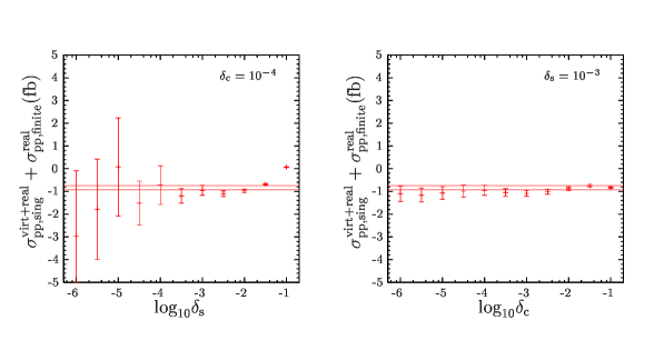
Figure 1: Dependence of the sum of the singular virtual corrections, the complete real corrections, and the term arising from the $\overline{\rm MS}$ definition of the PDFs for ${\mathrm{p}}{\mathrm{p}}\rightarrow\nu_{l}\bar{l}\gamma+X$ on the phase-space-slicing cut parameters. The horizontal lines indicate the error bars of our results obtained by using the subtraction method.

To check the treatment of the real corrections, we calculated the dependence of the sum of (2.16) and (2.17) on the slicing cut parameters $\delta_{\mathrm{s}}$ and $\delta_{\mathrm{c}}$ and compared the corresponding values to the sum of (2.22) and (2.31) obtained from the dipole subtraction method. In Figure 1 we show the dependence on $\delta_{\mathrm{s}}$ for fixed $\delta_{\mathrm{c}}=10^{-4}$ and the dependence on $\delta_{\mathrm{c}}$ for fixed $\delta_{\mathrm{s}}=10^{-3}$ for the process ${\mathrm{p}}{\mathrm{p}}\rightarrow\nu_{l}\bar{l}\gamma+X$. The error bars reflect the uncertainty of the Monte Carlo integration. The cross section shows a plateau over the full considered range for $\delta_{\mathrm{c}}$, whereas the variation with $\delta_{\mathrm{s}}$ leads to a plateau in the region $10^{-5}<\delta_{\mathrm{s}}<10^{-2}$. In addition, the numerical values obtained in these ranges agree with those obtained by using the subtraction method within the integration error, which we indicate in Figure 1 by the horizontal lines. The same analysis for the other considered processes yielded similar results. For the results to be presented in the next section, we accordingly fixed the slicing cuts to $\delta_{\mathrm{s}}=10^{-3}$ and $\delta_{\mathrm{c}}=10^{-4}$.

Finally, tree-level amplitudes and phase-space integration have been tested by comparing the outcome of our code with the results obtained with the program used for the analyses in Ref. [29]. This latter code employs matrix elements generated by means of PHACT[73], a set of routines based on the helicity-amplitude formalism of Ref. [74], and an independent integration method. For the sake of comparison, the original version of the program was extended to include the ${\mathrm{Z}}\gamma$-production processes (3.1) and (3.2). The results for all three Born cross sections agree at the per-mille level. Furthermore, we numerically cross-checked the lowest-order results for the distributions to be presented in the next section for all three processes. Complete agreement has been reached, which confirms our implementation of phase-space integration, cut routines, and histogram generation.

4 Numerical results

In this section, we illustrate the effect of the electroweak corrections on hadronic ${\mathrm{W}}\gamma$ and ${\mathrm{Z}}\gamma$ production at the LHC. For the process (3.1) we sum over all three neutrino flavours, while for the two processes (3.2) and (3.3) we include the first two lepton families only.

In the definition of the distributions for these processes, the possible presence of two photons in the final state, one coming from the real corrections, can lead to ambiguities. When observables of the final-state photon are involved, our prescription is to attribute the event weight to the bin corresponding to the photon with the largest energy.

4.1 Total cross sections

	$\sigma_{{\mathrm{p}}{\mathrm{p}}}^{(0)}$(fb)	$\sigma^{(1),{\rm tot}}_{{\mathrm{p}}{\mathrm{p}}}$(fb)		$1/\sqrt{2L\sigma^{(0)}_{{\mathrm{p}}{\mathrm{p}}}}\;(\%)$
$\nu_{l}\bar{\nu}_{l}\gamma$	$212.26(7)$	$-9.65(3)$	$-4.5\%$	$0.5\%$
$l\bar{l}\gamma$	$~{}38.99(9)$	$-2.61(7)$	$-6.7\%$	$1.1\%$
$\nu_{l}\bar{l}\gamma$	$124.57(8)$	$-2.36(5)$	$-1.9\%$	$0.6\%$

Table 1: Total lowest-order cross section (second column) as well as the electroweak ${\cal{O}}(\alpha)$ corrections in absolute size (third column) and in per cent of the lowest-order cross section (fourth column) for the three considered final states. The last column shows the statistical error for an integrated luminosity of $L=2\times 100/{\rm fb}$.

In Table 1, we show the total hadronic cross section for the three processes (3.1)–(3.3). The second column contains the lowest-order results, while the third and fourth entries display the value of the ${\cal{O}}(\alpha)$ corrections and their contribution relative to the lowest-order cross section, respectively. For the three considered processes, the electroweak corrections are negative and of the order of $-2\%$ to $-7\%$. This is to be compared with the last column of Table 1, where we show an estimate of the statistical error based on an integrated luminosity $L=100\,{\rm fb}^{-1}$ for two experiments. As can be seen, the size of the electroweak corrections well exceeds the statistical uncertainty. They are of the same order of magnitude as the systematic error, which is expected to be dominated by the error on the PDFs and thus presently of the order of 5% for processes initiated by quarks. The systematic uncertainty could possibly be reduced by considering ratios of cross sections. On the other hand, the size of the ${\cal{O}}(\alpha)$ corrections is strongly cut dependent and in fact increases with growing ${\mathrm{CM}}$ energy and vector-boson scattering angle. Larger values for the electroweak corrections are found by choosing, for instance, a more stringent cut on the transverse momentum of the photon. Such a constraint is useful for new-physics searches, although decreasing the statistics (see Ref. [29] and references therein). Also, distributions can be differently affected by the radiative corrections according to the specific observable at hand. In the following sections we illustrate this point for some sample variables.

4.2 Distributions for ${\mathrm{p}}{\mathrm{p}}\rightarrow\nu_{l}\bar{\nu}_{l}\gamma+X$

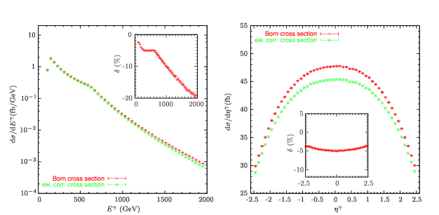
Figure 2: Distributions in energy (left plot) and rapidity (right plot) of the final-state photon for the process ${\mathrm{p}}{\mathrm{p}}\to\nu_{l}\bar{\nu_{l}}\gamma+X$, $l={\mathrm{e}},\mu,\tau$. The inserted plots show the relative ${\cal{O}}(\alpha)$ corrections in per cent normalized to the lowest order.

We begin by considering distributions for ${\mathrm{p}}{\mathrm{p}}\rightarrow\nu_{l}\bar{\nu}_{l}\gamma+X$. The error bars in the following plots result from the Monte Carlo integration errors. In the left plot of Figure 2, we show the energy distribution of the final-state photon. As previously mentioned, this distribution can be used to probe the existence of new particles which escape detection. These particles, once produced along with the photon, would lead to an excess of events in the high-energy domain. The kink at $E^{\gamma}=600\,\mathrm{GeV}$ is due to the cut $|\eta|<\eta^{\rm c}$ on the rapidity of the final-state photon. This cut restricts the cosine of the photon production angle $\theta^{\gamma}$ in the laboratory frame to the interval

$$\frac{\exp^{-2\eta^{\mathrm{c}}}-1}{\exp^{-2\eta^{\mathrm{c}}}+1}<\cos\theta^{\gamma}<\frac{\exp^{2\eta^{\mathrm{c}}}-1}{\exp^{2\eta^{\mathrm{c}}}+1},$$ (4.1)

such that for our choice $\eta^{\mathrm{c}}=2.5$:

$$\frac{p_{\rm T}^{\gamma}}{E^{\gamma}}=|\sin\theta^{\gamma}|>0.163071\ldots\approx\frac{1}{6}.$$ (4.2)

Since we also applied a cut of $p_{\rm T}^{\gamma,\mathrm{c}}=100\,\mathrm{GeV}$ on the transverse momentum of the photon, this condition is always fulfilled for $E^{\gamma}\mathrel{\raisebox{-3.00003pt}{$\stackrel{{\scriptstyle\displaystyle<}}{{\sim}}$}}600\,\mathrm{GeV}$ and the rapidity cut is never applied for these photon energies. For $E^{\gamma}\mathrel{\raisebox{-3.00003pt}{$\stackrel{{\scriptstyle\displaystyle>}}{{\sim}}$}}600\,\mathrm{GeV}$, on the other hand, the rapidity cut will start to exclude more and more events, which leads to a steeper decrease of the Born and NLO distributions. Assuming an LHC luminosity of $L=2\times 100/{\rm fb}$, the bin $E^{\gamma}=800\pm 10\,\mathrm{GeV}$ collects a contribution of ${\rm d}\sigma/{\rm d}E^{\gamma}\approx 5\times 10^{-2}\,{\rm fb}/{\rm GeV}$ to the total cross section, and will thus contain about

$$N_{\rm ev}\approx L\times\frac{{\rm d}\sigma}{{\rm d}E^{\gamma}}\Delta E^{\gamma}=200\,{\rm fb}^{-1}\times\frac{5\times 10^{-2}\,{\rm fb}}{{\rm GeV}}\,{20\,\mathrm{GeV}}=200$$ (4.3)

events, where $\Delta E^{\gamma}=20\;{\rm GeV}$ is the bin width. In this energy region, the electroweak corrections are of the order of $-10\%$. The increase of the corrections with $E^{\gamma}$ can be attributed to large logarithms of Sudakov type. The electroweak corrections should therefore be included to match the experimental accuracy. This is the first calculation of the ${\cal{O}}(\alpha)$ corrections to the photon spectrum for $\nu_{l}\bar{\nu_{l}}\gamma$ final states. Up to now, only QCD-corrected distributions have been computed. Since the electroweak corrections reduce cross sections and distributions, considering only lowest-order or QCD-corrected results could overestimate the SM background when looking for new particles. An excess of events in the high-energy domain could then be misinterpreted as compatible with the SM predictions, and could therefore be missed.

The right plot of Figure 2 shows the distribution in the photon rapidity. The electroweak corrections are here of the order of $-3\%$ to $-5\%$, and are thus smaller as in the case discussed above and of the order of the present systematic uncertainty from PDFs. This is because all bins receive the dominant contributions from events with low CM energies, where the electroweak corrections are small. An estimate of the event rate as in (4.3) applied to the bin $\eta^{\gamma}=0\pm 0.05$ gives 900 events.

4.3 Distributions for ${\mathrm{p}}{\mathrm{p}}\rightarrow l\bar{l}\gamma+X$

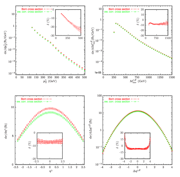
Figure 3: Distributions in the transverse momentum of the final-state photon (upper left plot), in the $\gamma{\mathrm{Z}}$ invariant mass (upper right plot), in the photon rapidity (lower left plot), and in the photon–${\mathrm{Z}}$-boson rapidity difference (lower right plot) for ${\mathrm{p}}{\mathrm{p}}\rightarrow l\bar{l}\gamma+X$, $l={\mathrm{e}},\mu$. The inserted plots show the relative ${\cal{O}}(\alpha)$ corrections in per cent normalized to the lowest order.

We turn now to the process (3.2), mediated by ${\mathrm{Z}}\gamma$ production, and we show in Figure 3 some sample distributions. The upper left plot displays the photon transverse momentum distribution. The kink at $p_{\rm T}^{\gamma}=250\,\mathrm{GeV}$ can be explained by the cut $\Delta R_{l\bar{l}}>R^{\mathrm{c}}$ on the rapidity-azimuthal angle separation of the two leptons resulting from the $\mathrm{Z}$ boson. The position of the kink is approximately given by

$$p_{\rm T}^{\gamma}=p_{\rm T}^{R^{\mathrm{c}}}\equiv\frac{2M_{\mathrm{Z}}}{\sqrt{\vphantom{A^{A}}2\exp(R^{\mathrm{c}})-1}-1}.$$ (4.4)

For $p_{\rm T}^{{\mathrm{Z}}}=p_{\rm T}^{\gamma}<p_{\rm T}^{R^{\mathrm{c}}}$ the $R^{\mathrm{c}}$ cut is not effective, while for $p_{\rm T}^{{\mathrm{Z}}}=p_{\rm T}^{\gamma}>p_{\rm T}^{R^{\mathrm{c}}}$ the decay products of the ${\mathrm{Z}}$ boson are so strongly boosted that this cut eliminates many of the events. The effects of the electroweak corrections to this distribution have already been studied in Ref. [30] for an on-shell final-state ${\mathrm{Z}}$ boson, and with the real corrections included in the soft and collinear limits only. In this case, the corrections were found to be large and negative, of the order of $-20\%$ and to increase in absolute size with rising $p_{\rm T}^{\gamma}$. As can be seen from Figure 3, our calculation largely confirms these results. Since the effects of the anomalous couplings are most pronounced in the high-$p_{\rm T}$ region, the electroweak corrections could modify the experimental sensitivity to possible new physics. For the process considered here, the QCD corrections to the distribution in the photon transverse momentum have been calculated in Refs. [18, 19, 21]. If applying a jet veto, they are found to range between $+60\%$ and $-20\%$ [21]. At NLO, the contributions arising from electroweak and QCD corrections are thus comparable in magnitude. Including the electroweak radiative effects in the experimental analysis is therefore mandatory in order not to overestimate the SM background.

In the upper right plot of Figure 3, we show the distribution in the final-state invariant mass. A simple estimate as in (4.3) shows that the process should be observable up to $M_{\rm inv}^{\gamma{\mathrm{Z}}}=750$–$1000\,\mathrm{GeV}$. As can be seen from the inset plot, the total electroweak corrections amount to roughly $-8\%$, independently of the $M_{\rm inv}^{\gamma{\mathrm{Z}}}$ value. Electroweak radiative-correction effects are thus relevant for this important distribution. Earlier results for the electroweak corrections to the invariant-mass distribution have been published in Ref. [30] under the aforementioned approximations. Large negative corrections of the order of $-15\%$ were found, increasing in magnitude towards larger invariant masses. Comparing these results to the curve shown in the inset of the upper right plot in Figure 3, we rather find the relative size of the virtual and real corrections approaching a plateau with rising invariant mass. We attribute this effect to angular-dependent logarithms, which are enhanced for events with photons collinear to the beams and compensate the Sudakov logarithms. Such events are eliminated by a cut on $p_{\rm T}^{\gamma}$ and thus do not influence the $p_{\rm T}^{\gamma}$ distribution, but contribute to the invariant-mass distribution also for large invariant masses. Thus, compared to the results published in Ref. [30], the inclusion of the real corrections reduces the impact of the electroweak corrections for large invariant masses.

The distribution in the photon rapidity is shown in the lower left plot of Figure 3. The relative size of the electroweak corrections can be seen from the inserted plot to be of the order of $-7\%$. Finally, the photon–${\mathrm{Z}}$-boson rapidity difference is shown in the lower right plot of Figure 3. While the corresponding corrections are at a similar level as for the two previous distributions in the central region, they become large and positive near $|\Delta\eta^{\gamma{\mathrm{Z}}}|\approx 4$. For $|\Delta\eta^{\gamma{\mathrm{Z}}}|>5$, the cut $|\eta^{\gamma}|<\eta^{\mathrm{c}}=2.5$ eliminates all events with only one photon and a pair of leptons in the final state, and only bremsstrahlung events contribute. Thus, the smallness of the lowest order cross section causes the large relative corrections near and above $|\Delta\eta^{\gamma{\mathrm{Z}}}|\approx 4$. However, the event rate expected at the LHC in this region is too small for experimental observation. The remaining central part of the curve does not present novelties compared to the two previous distributions.

4.4 Distributions for ${\mathrm{p}}{\mathrm{p}}\rightarrow{\nu}_{l}\bar{l}\gamma+X$

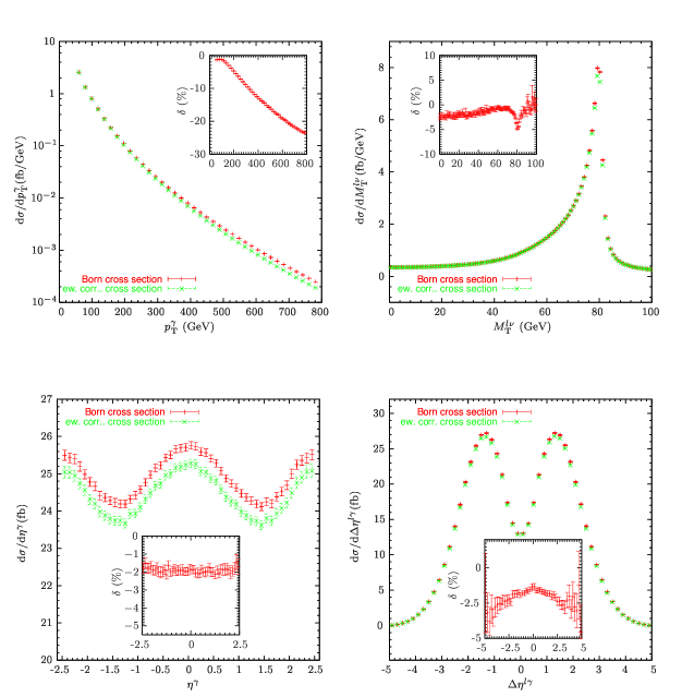
Figure 4: Distributions in the transverse momentum of the final-state photon (upper left plot), in the transverse mass of the lepton–neutrino pair (upper right plot), in the photon rapidity (lower left plot) and in the lepton–photon rapidity difference (lower right plot) for ${\mathrm{p}}{\mathrm{p}}\rightarrow\nu_{l}\bar{l}\gamma+X$, $l={\mathrm{e}},\mu$. The inserted plots show the relative electroweak corrections in per cent normalized to the lowest order.

Turning next to the ${\mathrm{W}}\gamma$ production process, we show in Figure 4 some distributions for ${\mathrm{p}}{\mathrm{p}}\rightarrow{\nu}_{l}\bar{l}\gamma+X$, $l={\mathrm{e}},\mu$. Starting with the transverse-momentum distribution of the photon in the upper left plot, an estimate as in (4.3) shows that the event rate should be observable up to $p_{\rm T}^{\gamma}=300$–$400\,\mathrm{GeV}$. An analysis of the effects of the electroweak corrections on this distribution summed over $\nu_{l}\bar{l}$ and $l\bar{\nu}_{l}$ final states has already been published in Ref. [29], taking into account the ${\mathrm{W}}$-boson decay but including only the leading logarithmic virtual corrections to the production subprocess in the high-energy approximation. Large negative corrections were found, which can reach up to $-12\%$ at $p_{\rm T}^{\gamma}=400\,\mathrm{GeV}$. As can be seen from the inset plot, we reproduce this result. At $p_{\rm T}^{\gamma}=400\,\mathrm{GeV}$, the electroweak corrections are found to contribute about $-13\%$ of the Born result, which is well above the systematic and statistical errors. The QCD corrections to the transverse-momentum distribution of the photon have been analysed in Ref. [21]. If applying a jet veto, large positive corrections of up to $60\%$ for low transverse momenta have been found. They decrease to $-5\%$ to $-10\%$ of the Born cross section at $p_{\rm T}^{\gamma}=400\,\mathrm{GeV}$. For high transverse momenta, the electroweak corrections are thus of the same order of magnitude or even larger than the QCD corrections, and further reduce the lowest-order distribution. Again, a data analysis performed just including QCD corrections could overestimate the SM background in anomalous coupling measurements.

In the upper right plot of Figure 4, we display our results for the distribution in the transverse mass of the final-state lepton–neutrino pair as defined in (3.19). The curves terminate at the cut value $M_{\rm T,c}^{l\nu}=M_{\mathrm{W}}+20\;{\rm GeV}\approx 100.4\,\mathrm{GeV}$. The ${\mathrm{W}}$-boson resonance can be observed as a pronounced peak, an effect which could be used to determine the ${\mathrm{W}}$-boson mass as a consistency check. The electroweak corrections can be seen from the inserted plot to contribute most at the peak, where they amount to $-4\%$ of the Born cross section.

An interesting property of angular distributions for ${\mathrm{W}}\gamma$ pair production is the radiation zero, i.e. a kinematical configuration where all tree-level helicity amplitudes of the parton process are exactly zero. The radiation zero appears at

$$\cos\hat{\theta}^{\gamma}=\frac{Q_{\mathrm{u}}+Q_{\mathrm{d}}}{Q_{\mathrm{u}}-Q_{\mathrm{d}}}=\frac{1}{3},$$ (4.5)

where $\hat{\theta}$ is the scattering angle of the photon in the partonic CM frame, and $Q_{\mathrm{u}}$ and $Q_{\mathrm{d}}$ denote the charge of the up quark and down quark, respectively. At the LHC, the radiation zero should be observable as a dip in the distribution in the rapidity difference between the photon and the charged lepton coming from the ${\mathrm{W}}$ boson [3, 21]. It arises from gauge cancellations, and is characteristic for the SM. As a consequence, deviations from the SM gauge structure generally tend to fill in the dip, such that an analysis of the radiation zero provides an excellent opportunity to probe new physics. QCD corrections generally enhance the cross section at the radiation zero [3]. Depending on the process definition, the effect can be quite dramatic. If no jet veto is applied, the dip arising from the radiation zero is completely washed out. If selecting only events without final-state jets, a dip at the level of 20% survives. In the bottom right plot of Figure 4, we display our results for the distribution in the rapidity difference between the photon and the charged lepton, which exhibits the dip originating from the radiation zero at $\Delta\eta^{l\gamma}\approx 0$. The electroweak corrections hardly influence the dip and amount to about $-2\%$. This is probably too small to have an observable impact on the data analysis. The smallness of the ${\cal{O}}(\alpha)$ correction has again its origin in the fact that a given bin receives the main contributions from the low-energy domain of phase-space, where the electroweak corrections are small. Selecting kinematical regions characterized by larger energies and scattering angles would increase the size of the electroweak corrections, at the same time enhancing the radiation zero dip, as shown in Ref. [29], but decrease the statistics.

Analogous remarks apply to the electroweak corrections to the photon-rapidity distribution shown in the bottom left of Figure 4. The central peak in this distribution is caused by events with small $p^{\gamma}_{\mathrm{T}}$ and disappears if the cut $p^{\gamma,\mathrm{c}}_{\mathrm{T}}=50\,\mathrm{GeV}$ is increased. The peaks in forward and backward direction are also present for larger $p^{\gamma,\mathrm{c}}_{\mathrm{T}}$. They result from the peaking of the partonic matrix element in the direction of the incoming up quark which is additionally amplified by the boost from the CM to the laboratory system, which goes preferably along the direction of the valence quark.

4.5 Comparison with virtual correction in high-energy approximation

It is interesting to compare our results for the electroweak corrections to hadronic ${\mathrm{W}}\gamma$ production with those obtained in Ref. [29]. In this latter calculation, the virtual corrections were determined for the production subprocess only, and using the High-Energy Approximation (HEA) of Refs. [75, 76, 77]. In this approximation, all terms that vanish with $M_{\mathrm{W}}/\sqrt{\hat{s}}$ at high energies are neglected, and only the logarithmic contributions to the loop integrals of the form $\ln^{2}(\hat{s}/M_{\mathrm{W}}^{2})$, $\ln(\hat{s}/M_{\mathrm{W}}^{2})\ln(\hat{s}/\hat{x})$ and $\ln(\hat{s}/M_{\mathrm{W}}^{2})$ are taken into account, where $\hat{x}=\hat{t},\hat{u}$ denotes one of the Mandelstam variables for the production subprocess. The use of the HEA is justified by requiring a large transverse momentum of the final-state photon, which results in large values for the partonic CM energy $\sqrt{\hat{s}}$ compared to the ${\mathrm{W}}$-boson mass, and thus to large values for the above logarithms.

In order to tune our results to those of Ref. [29], we generated the amplitudes for the virtual corrections using Pole, but we switched off the diagrams involving the corrections to the decay subprocess. We evaluated the so-obtained amplitudes numerically by adapting the input to the parameter and cut values used in Ref. [29]. For this comparison, we moreover summed up the process (3.3) and its charge-conjugate, i.e. we considered both ${\mathrm{W}}^{+}\gamma$ and ${\mathrm{W}}^{-}\gamma$ production. The resulting numerical values for the Born cross section and the finite virtual corrections are shown in Table 2 for some values of the cut on the transverse momentum of the final-state photon. The numbers in parentheses represent the integration errors in the last digits. Note that the values shown in Table 2 do not exactly correspond to the results presented in a similar table in Ref. [29]. This is because we found an error in the implementation of the azimuthal-pseudorapidity separation (3.15) when comparing our results to those of Ref. [29].

	Ref. [29]			this work
$p_{\rm T}^{\gamma,{\rm c}}({\rm GeV})$	$\sigma_{{\mathrm{p}}{\mathrm{p}}}^{(0)}({\rm fb})$	$\sigma_{{{\mathrm{p}}{\mathrm{p}},\rm finite}}^{{\rm virt}}({\rm fb})$	$\delta_{{{\mathrm{p}}{\mathrm{p}},\rm finite}}^{{\rm virt}}$	$\sigma^{(0)}_{{\mathrm{p}}{\mathrm{p}}}({\rm fb})$	$\sigma_{{{\mathrm{p}}{\mathrm{p}},\rm finite}}^{{\rm virt}}({\rm fb})$	$\delta_{{{\mathrm{p}}{\mathrm{p}},\rm finite}}^{{\rm virt}}$
250	$6.01~{}$	$-0.292$	$-4.86\%$	$6.02(3)$	$-0.649(3)$	$-10.8\%$
450	$0.712$	$-9.78\times 10^{-2}$	$-13.74\%$	$0.711(4)$	$-0.1372(7)$	$-19.3\%$
700	$9.30\times 10^{-2}$	$-2.06\times 10^{-2}$	$-22.12\%$	$9.31(6)\times 10^{-2}$	$-2.54(2)\times 10^{-2}$	$-27.3\%$
1000	$1.25\times 10^{-2}$	$-3.72\times 10^{-3}$	$-29.6\%$	$1.253(9)\times 10^{-2}$	$-4.32(3)\times 10^{-3}$	$-34.5\%$

Table 2: Lowest-order cross section and finite virtual corrections to the production subprocess for ${\mathrm{p}}{\mathrm{p}}\rightarrow{\mathrm{W}}^{\pm}\gamma+X\rightarrow l\nu_{l}\gamma+X$, where $l\nu_{l}=l\bar{\nu}_{l}+\bar{l}\nu_{l}$ and $l=e,\mu$.

The results for the Born cross section agree within errors at the per-mille level. Comparing our results for the finite virtual corrections to those obtained in the HEA in Ref. [29], one would expect a sizeable difference for low $p_{\rm T}^{\rm\gamma,\mathrm{c}}$ values, which decreases for higher values of this cut to the level of $1$–$2\%$. However, the numbers in Table 2 point rather towards a constant difference of approximately $5$–$6\%$.

In order to understand this effect, we used the fact that Pole employs the FF-based package LoopTools [78, 79], which numerically reduces all tensorial loop integrals onto a set of scalar basis integrals. We replaced each loop integral in this basis set by the corresponding expression in the HEA, and split the latter into different contributions. The total electroweak corrections obtained in this way are smaller than those in Table 2 by at most half a per cent. The subcontributions obtained with this procedure are shown in Table 3.

$p_{\rm T}^{\gamma,\rm c}({\rm GeV})$	$\sigma^{(1)}_{{\rm EWLog}}({\rm fb})$	$\delta^{(1)}_{{\rm EWLog}}$	$\Delta\sigma^{(1)}_{{\rm QED}}({\rm fb})$	$\delta^{(1)}_{{\rm QED}}$	$\sigma^{(1)}_{{\rm rem}}({\rm fb})$	$\delta^{(1)}_{{\rm rem}}$
250	$-0.364(1)$	$-6.05\%$	$8.6(1)\times 10^{-2}$	$1.43\%$	$-0.360(2)$	$-5.99\%$
450	$-0.1026(4)$	$-14.4\%$	$1.13(2)\times 10^{-2}$	$1.59\%$	$-4.29(2)\times 10^{-2}$	$-6.04\%$
700	$-2.11(1)\times 10^{-2}$	$-22.6\%$	$1.40(3)\times 10^{-3}$	$1.50\%$	$-5.31(3)\times 10^{-3}$	$-5.71\%$
1000	$-3.77(3)\times 10^{-3}$	$-30.1\%$	$1.74(5)\times 10^{-4}$	$1.39\%$	$-6.63(5)\times 10^{-4}$	$-5.29\%$

Table 3: Finite virtual corrections to the production subprocess for ${\mathrm{p}}{\mathrm{p}}\rightarrow{\mathrm{W}}^{\pm}\gamma+X\rightarrow l\nu_{l}\gamma+X$ in HEA split into electroweak logarithmic contributions $\sigma^{(1)}_{{\rm EWLog}}$, the QED remnants $\Delta\sigma^{(1)}_{{\rm QED}}$, as well as the remaining contributions $\sigma^{(1)}_{{\rm rem}}$.

The electroweak logarithmic contributions in the second and third column of Table 3 result from the contributions to the basic loop integrals that involve only logarithms of the form $\ln^{2}(\hat{s}/M_{\mathrm{W}}^{2})$, $\ln(\hat{s}/M_{\mathrm{W}}^{2})\ln(\hat{s}/\hat{x}),$ $x=\hat{t},\hat{u}$ and $\ln(\hat{s}/M_{\mathrm{W}}^{2})$. This is the approximation used in Ref. [29]. As can be seen by comparing these numbers to the results in the third and fourth column in Table 2, the leading logarithmic contributions differ by about $1.2\%$ for $p_{\rm T}^{\gamma,\mathrm{c}}=250\,\mathrm{GeV}$ and this difference decreases to the per-mille level for higher cut values. Thus we can reproduce the results of Ref. [29] to a satisfying accuracy by keeping only the electroweak logarithms.

The QED contributions in the fourth and fifth column of Table 3 are obtained by keeping only terms involving logarithms in the regulators for the masses of the photon and the external light fermions, i.e. logarithms of the form $\ln(m_{\gamma}^{2}/M_{\mathrm{W}}^{2})$ or $\ln(m_{i}^{2}/M_{\mathrm{W}}^{2})$, in the loop integrals and subtracting the finite virtual corrections as given in (2.39). We here observe a roughly energy-independent contribution of about $1.5\%$. This contribution results from the fact that the subtraction term (2.39) involves logarithms of the form $\ln(m_{\gamma}^{2}/s_{ij})$ and $\ln(m_{i}^{2}/s_{ij})$ while in the HEA they appear as $\ln(m_{\gamma}^{2}/M_{\mathrm{W}}^{2})$ and $\ln(m_{i}^{2}/M_{\mathrm{W}}^{2})$.

Finally, the contributions listed in the sixth and seventh column of Table 3 result from all remaining terms in the HEA, i.e. logarithms depending only on ratios of kinematical variables and constant terms in the high-energy expressions of the basic loop integrals, as well as extra constant terms arising from the reduction of tensor loop integral to scalar loop integrals. These remaining terms yield a contribution of $5$–$6\%$ and thus make up the largest part of the difference between our results and those of Ref. [29].

In order to trace the origin of this large effect, we further split the remaining contributions to the basic loop integrals as shown in Table 4.

$p_{\rm T}^{\rm c}({\rm GeV})$	$\sigma^{(1)}_{{\rm rem,NoLog}}({\rm fb})$	$\delta^{(1)}_{{\rm rem,NoLog}}$	$\sigma^{(1)}_{{\rm rem,Log}}({\rm fb})$	$\delta^{(1)}_{{\rm rem,Log}}$	$\sigma^{(1)}_{{\rm rem,Log}^{2}}({\rm fb})$	$\delta^{(1)}_{{\rm rem,Log}^{2}}$
250	$-1.55(8)\times 10^{-2}$	$-0.26\%$	$-0.107(1)$	$-1.78\%$	$-0.238(2)$	$-3.95\%$
450	$-4.13(8)\times 10^{-3}$	$-0.58\%$	$1.139(2)\times 10^{-2}$	$-1.97\%$	$-2.48(2)\times 10^{-2}$	$-3.50\%$
700	$-6.94(9)\times 10^{-4}$	$-0.74\%$	$-1.78(2)\times 10^{-3}$	$-1.91\%$	$-2.83(2)\times 10^{-3}$	$-3.05\%$
1000	$-1.09(1)\times 10^{-4}$	$-0.87\%$	$-2.25(3)\times 10^{-4}$	$-1.79\%$	$-3.29(3)\times 10^{-4}$	$-2.62\%$

Table 4: The non-leading contributions to the virtual corrections to the production subprocess for ${\mathrm{p}}{\mathrm{p}}\rightarrow{\mathrm{W}}^{\pm}\gamma+X\rightarrow l\nu_{l}\gamma+X$ in HEA split up into terms $\sigma^{(1)}_{{\rm rem,NoLog}}$ containing no angular-dependent logarithms, into terms $\sigma^{(1)}_{{\rm rem,Log}}$ depending on single angular-dependent logarithms as well as into terms $\sigma^{(1)}_{{\rm rem,Log}^{2}}$ depending on angular-dependent logarithms squared.

The numbers in the fourth and fifth column comprise the contributions linear in the purely angular-dependent logarithms, i.e. logarithms of the form $\ln(\hat{s}/\hat{x}),$ $x=\hat{t},\hat{u}$, whereas the numbers in the sixth and seventh column correspond to the terms containing these logarithms squared. As can be seen from Table 4, the contributions linear and quadratic in the purely angular-dependent logarithms vary only little with increasing energy, but contribute with about $-2\%$ and $-(3$–$4)\%$, respectively, i.e. the make up the bulk of the remaining contributions. The large size of the contributions of the purely angular-dependent logarithms can be explained by the enhancement of the cross section of the considered processes in the forward and backward directions. Since in these regions $\hat{s}/\hat{t}$ or $\hat{s}/\hat{u}$ are small the purely angular-dependent logarithms become large. The contributions of these logarithms are the source of comparably large difference between the corrections in the HEA of Ref. [29] and the results of this paper. On the other hand, as shown in the second and third column of Table 4 the non-logarithmic remaining terms contribute to the cross section only below the per-cent level. The increase of this contribution with rising transverse momentum cut of the photon can be attributed to the energy dependence of those parts of the matrix elements that have not been evaluated in the HEA.

We thus find that, for processes dominated by contributions coming from phase-space regions with small kinematical variables, the accuracy of the HEA which only takes into account enhanced logarithms of $\hat{s}/M^{2}$ may only be at the level of several per cent, unless the enhanced angular-dependent logarithms are included as well.

5 Summary and Conclusions

We have calculated the electroweak corrections to ${\mathrm{Z}}\gamma$ and ${\mathrm{W}}\gamma$ production at the LHC, with ${\mathrm{Z}}$ and ${\mathrm{W}}$ decaying into leptons. For the Born cross sections and the real corrections we use complete matrix elements. The virtual corrections are included in the leading-pole approximation. For a treatment of the soft and collinear divergences, we used the dipole subtraction method as well as the phase-space-slicing technique.

We have implemented our strategy in a Mathematica package called Pole, which works as an extension of the programs FeynArts3 and FormCalc3.1 and is designed to calculate electroweak corrections in leading-pole approximation for hadronic or partonic processes. We have applied the program to the ${\mathrm{p}}{\mathrm{p}}\rightarrow\nu_{l}\bar{\nu_{l}}\gamma,l\bar{l}\gamma,\nu_{l}\bar{l}\gamma$ processes at the LHC, and tested the results extensively. As part of our checks we have performed a comparison with the virtual corrections evaluated in the high-energy approximation, which reveals that angular-dependent logarithms can give effects of several per cent at high energies.

For the above-mentioned processes and typical LHC cuts, we find electroweak corrections of the order of $-5\%$ for total cross sections and angular distributions as, for instance, the radiation zero in ${\mathrm{W}}\gamma$ production. For transverse-momentum and energy distributions, the ${\cal{O}}(\alpha)$ corrections contribute up to $-20\%$ of the lowest-order cross section. Their influence is thus well above the systematic and statistical errors, and may be of the same size as the QCD corrections or even larger, depending on the cut settings. Consequently, electroweak radiative effects have to be included in the experimental analysis when looking for the existence of anomalous vector-boson couplings or for the production of new particles via hadronic production of ${\mathrm{Z}}\gamma$ and ${\mathrm{W}}\gamma$. Thus, the Monte Carlo generators for LHC should include besides QCD corrections also the electroweak corrections.

Appendix A Analytical results for the amplitudes

In this appendix, we summarize analytical results for those parts of the amplitudes that are compact enough to be explicitly displayed. We present the analytical expressions for the Born amplitude in Section A.1, the amplitude corresponding to the non-factorizable corrections in Section A.2, and the amplitudes for the QED bremsstrahlung processes in Section A.3. The calculation of the Born and bremsstrahlung amplitudes are carried out in the framework of the Weyl–van der Waerden formalism [80, 81] as presented in Ref. [82].

A.1 The Lowest-order amplitudes

The helicity amplitudes of all partonic processes (2.4) can be obtained from the generic set of Feynman diagrams shown in Figure 5.

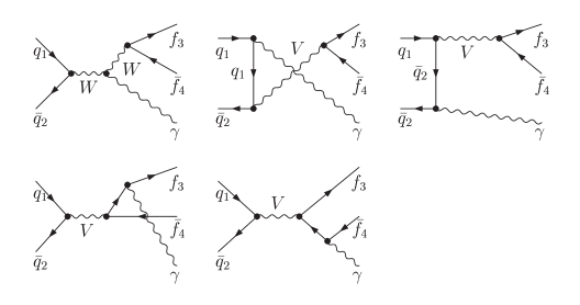
Figure 5: Tree-level diagrams for $q_{1}+\bar{q}_{2}\rightarrow f_{3}+\bar{f}_{4}+\gamma$

The amplitude corresponding to these diagrams can be written as

$${\cal M}^{(0)\;\sigma_{1}\sigma_{2}\sigma_{3}\sigma_{4}\lambda_{5}}_{\;\;c_{1}c_{2}}(p_{1},p_{2},p_{3},p_{4},p_{5})=-2\sqrt{2}e^{3}\delta_{c_{1}c_{2}}\delta_{\sigma_{1}-\sigma_{2}}\delta_{\sigma_{3}-\sigma_{4}}\\ \sum_{V}C^{\sigma_{1}}_{V\bar{q}_{2}q_{1}}C^{\sigma_{3}}_{V\bar{f}_{3}f_{4}}{\rm B}_{V}^{\sigma_{1}\sigma_{3}\lambda_{5}}(p_{1},p_{2},p_{3},p_{4},p_{5},Q_{q_{1}},Q_{{q}_{2}},Q_{f_{3}},Q_{{f}_{4}}),$$ (A.1)

where the quantities $Q_{i},i=1,\ldots 4$ denote the charges of the external fermions (the charges of the external antifermions are given by $-Q_{i}$.) and $c_{1},c_{2}$ are the colour indices for the initial-state quarks. The sum over $V$ runs over all SM vector bosons. The non-vanishing gauge couplings $C^{\pm}_{V\bar{f}_{a}f_{b}}$ of a fermion $f_{b}$ and an anti-fermion $\bar{f}_{a}$ to the vector boson $V$ are listed in Table 5 using the following conventions.

$C^{\pm}_{\gamma\bar{f_{2}}f_{1}}$	$=$	$-Q_{f_{1}}\delta_{f_{1}f_{2}},$	$f_{1,2}=q,l$
$C^{\sigma}_{Z\bar{f}_{2}f_{1}}$	$=$	$\left\{\begin{array}[]{l c l}-\frac{s_{\mathrm{w}}}{c_{\mathrm{w}}}Q_{f_{1}}\delta_{f_{1}f_{2}},&&{\rm for}\;\sigma=+\\[4.30554pt] \frac{I^{3}_{f_{1}}-s_{\mathrm{w}}^{2}Q_{f_{1}}}{s_{\mathrm{w}}c_{\mathrm{w}}}\delta_{f_{1}f_{2}},&&{\rm for}\;\sigma=-\end{array}\right.,$	$f_{1,2}=q,l$
$C^{\sigma}_{W^{-}\bar{l}\nu_{l}}$	$=$	$\left\{\begin{array}[]{l c l}\hbox to0.0pt{0,\hss}\hphantom{\frac{I^{3}_{f_{1}}-s_{\mathrm{w}}^{2}Q_{f_{1}}}{s_{\mathrm{w}}c_{\mathrm{w}}}\delta_{f_{1}f_{2}},}&&{\rm for}\;\sigma=+\\[4.30554pt] \frac{1}{\sqrt{2}s_{\mathrm{w}}},&&{\rm for}\;\sigma=-\end{array}\right.,$	$l={\mathrm{e}},\mu,\tau$
$C^{\sigma}_{W^{+}\bar{\nu}_{l}l}$	$=$	$\left\{\begin{array}[]{l c l}\hbox to0.0pt{0,\hss}\hphantom{\frac{I^{3}_{f_{1}}-s_{\mathrm{w}}^{2}Q_{f_{1}}}{s_{\mathrm{w}}c_{\mathrm{w}}}\delta_{f_{1}f_{2}},}&&{\rm for}\;\sigma=+\\[4.30554pt] \frac{1}{\sqrt{2}s_{\mathrm{w}}},&&{\rm for}\;\sigma=-\end{array}\right.,$	$l={\mathrm{e}},\mu,\tau$
$C^{\sigma}_{W^{-}\bar{q}_{2}q_{1}}$	$=$	$\left\{\begin{array}[]{l c l}\hbox to0.0pt{0,\hss}\hphantom{\frac{I^{3}_{f_{1}}-s_{\mathrm{w}}^{2}Q_{f_{1}}}{s_{\mathrm{w}}c_{\mathrm{w}}}\delta_{f_{1}f_{2}},}&&{\rm for}\;\sigma=+\\[4.30554pt] \frac{1}{\sqrt{2}s_{\mathrm{w}}}V_{q_{2}q_{1}}^{\dagger},&&{\rm for}\;\sigma=-\end{array}\right.,$	$q_{1}={\mathrm{u}},{\mathrm{c}},{\mathrm{t}},\quad q_{2}={\mathrm{d}},{\mathrm{s}},{\mathrm{b}}$
$C^{\sigma}_{W^{+}\bar{q}_{2}q_{1}}$	$=$	$\left\{\begin{array}[]{l c l}\hbox to0.0pt{0,\hss}\hphantom{\frac{I^{3}_{f_{1}}-s_{\mathrm{w}}^{2}Q_{f_{1}}}{s_{\mathrm{w}}c_{\mathrm{w}}}\delta_{f_{1}f_{2}},}&&{\rm for}\;\sigma=+\\[4.30554pt] \frac{1}{\sqrt{2}s_{\mathrm{w}}}V_{q_{2}q_{1}},&&{\rm for}\;\sigma=-\end{array}\right.,$	$q_{1}={\mathrm{d}},{\mathrm{s}},{\mathrm{b}},\quad q_{2}={\mathrm{u}},{\mathrm{c}},{\mathrm{t}}$

Table 5: Coupling constants of quarks and leptons to the gauge bosons $V=\gamma,Z,W^{\pm}$

The particle indices $l$ ($q$) denote leptons (quarks). The charges and the third component of the isospin of the fermion $f$ are denoted by $Q_{f}$ and $I^{3}_{f}$, respectively. The quantities $s_{\mathrm{w}}$ and $c_{\mathrm{w}}$ are the sine and the cosine of the weak mixing angle, whereas $\alpha$ is the fine-structure constant. Finally, $\delta_{ij}$ and $V_{ij}$ denote the Kronecker delta and the quark mixing matrix. Note, that the elementary charge $e$ has been extracted from the couplings.

As discussed in Section 2.3, the amplitude can be split into a resonant and a non-resonant part. This splitting can be done on the level of the generic functions

$${\rm B}_{V}^{\sigma_{1}\sigma_{3}\lambda_{5}}={\rm B}_{V}^{{\rm res},\sigma_{1}\sigma_{3}\lambda_{5}}+{\rm B}_{V}^{{\rm nres},\sigma_{1}\sigma_{3}\lambda_{5}}.$$ (A.2)

The resonant part comprises all contributions from diagrams containing the resonant propagator of the decaying particle $V$, and thus corresponds to the amplitude originating from the diagrams in the first row of Figure 5. Applying the Weyl–van der Waerden formalism as presented in Ref. [82] to these diagrams, the generic function for all helicities positive is given by

$${\rm B}_{V}^{{\rm res},+++}(p_{1},p_{2},p_{3},p_{4},p_{5},Q_{1},Q_{2},Q_{3},Q_{4})=-P_{V}(p_{3}+p_{4})\frac{\langle p_{1}p_{4}\rangle^{2}}{\langle p_{4}p_{5}\rangle}\\ \times\left\{\frac{Q_{1}\langle p_{3}p_{2}\rangle^{\star}}{\langle p_{1}p_{5}\rangle}+\frac{Q_{2}\langle p_{3}p_{1}\rangle^{\star}}{\langle p_{2}p_{5}\rangle}-(Q_{2}-Q_{1})P_{V}(p_{1}+p_{2})\langle p_{3}p_{5}\rangle^{\star}\langle p_{2}p_{1}\rangle^{\star}\right\}.$$ (A.3)

The non-resonant part of the Born amplitude, on the other hand, receives contributions from the remaining diagrams in the second row of Figure 5. Expressed in Weyl-spinor products, the generic function for all helicities positive reads

$${\rm B}_{V}^{{\rm nres},+++}(p_{1},p_{2},p_{3},p_{4},p_{5},Q_{1},Q_{2},Q_{3},Q_{4})=P_{V}(p_{1}+p_{2})\frac{Q_{3}\langle p_{1}p_{4}\rangle^{2}\langle p_{2}p_{1}\rangle^{\star}}{\langle p_{3}p_{5}\rangle\langle p_{4}p_{5}\rangle}.$$ (A.4)

Here $M_{V}$ is the mass and $\Gamma_{V}$ the decay width of the vector boson $V$, and the corresponding propagators are denoted as

$$P_{V}(k)=\frac{1}{k^{2}-M_{V}^{2}-{\mathrm{i}}M_{V}\Gamma_{V}}.$$ (A.5)

The Weyl-spinor products are defined by

$$\langle pq\rangle=2\sqrt{p_{0}q_{0}}\,\Biggl{[}{\mathrm{e}}^{-{\mathrm{i}}\phi_{p}}\cos\frac{\theta_{p}}{2}\sin\frac{\theta_{q}}{2}-{\mathrm{e}}^{-{\mathrm{i}}\phi_{q}}\cos\frac{\theta_{q}}{2}\sin\frac{\theta_{p}}{2}\Biggr{]},$$ (A.6)

where $\theta_{p}$, $\theta_{q}$ and $\phi_{p}$, $\phi_{q}$ are the polar and azimuthal angles, respectively, of the corresponding light-like 4-momenta

$$p^{\mu} = p_{0}(1,\sin\theta_{p}\cos\phi_{p},\sin\theta_{p}\sin\phi_{p},\cos\theta_{p}),$$

$$q^{\mu} = q_{0}(1,\sin\theta_{q}\cos\phi_{q},\sin\theta_{q}\sin\phi_{q},\cos\theta_{q}).$$ (A.7)

The amplitudes for neutral current reactions can be extracted from (A.3) and (A.4) by simply setting $(Q_{2}-Q_{1})=0$. Inserting (A.3) and (A.4) in (A.1) and adding the resulting expressions yields the full Born amplitude. While this is gauge invariant, the resonant and non-resonant parts as defined above are gauge-dependent, unless applying the LPA. To this end, one has to set the finite width in the $s$-channel propagator $P_{V}(p_{1}+p_{2})$ in the resonant amplitude (A.3) to zero and to insert the resulting expression in (A.1), where the spinor and scalar products have to be evaluated using the on-shell projected momenta, except for in the resonant propagator $P_{V}(p_{3}+p_{4})$. Note that we set the gauge spinor for the external photon to $g=p_{4}$ to obtain the above results, which is why the contribution of the diagram with the photon coupling to the external fermion $f_{4}$ vanishes.

Dropping the superscript for resonant and non-resonant contributions in what follows, the other helicity combinations can be obtained as

$${\rm B}_{V}^{-++}(p_{1},p_{2},p_{3}, \,p_{4},p_{5},Q_{1},Q_{2},Q_{3},Q_{4})$$

$$={\rm B}_{V}^{+++}(p_{2},p_{1},p_{3},p_{4},p_{5},-Q_{2},-Q_{1},Q_{3},Q_{4}),$$

$${\rm B}_{V}^{+-+}(p_{1},p_{2},p_{3}, \,p_{4},p_{5},Q_{1},Q_{2},Q_{3},Q_{4})$$

$$={\rm B}_{V}^{+++}(p_{1},p_{2},p_{4},p_{3},p_{5},Q_{1},Q_{2},-Q_{4},-Q_{3}),$$

$${\rm B}_{V}^{--+}(p_{1},p_{2},p_{3}, \,p_{4},p_{5},Q_{1},Q_{2},Q_{3},Q_{4})$$

$$={\rm B}_{V}^{+++}(p_{2},p_{1},p_{4},p_{3},p_{5},-Q_{2},-Q_{1},-Q_{4},-Q_{3}),$$ (A.8)

as well as

$${\rm B}_{V}^{\sigma_{1}\sigma_{3}-}(p_{1},p_{2},p_{3},p_{4},p_{5},Q_{1},Q_{2},Q_{3},Q_{4})\\ =\left[{\rm B}_{V}^{-\sigma_{1}-\sigma_{3}+}(p_{1},p_{2},p_{3},p_{4},p_{5},Q_{1},Q_{2},Q_{3},Q_{4})\right]^{\star}\Bigg{|}_{P_{V}^{\star}\rightarrow P_{V}}.$$ (A.9)

A.2 The non-factorizable corrections

A general discussion for the photonic non-factorizable corrections for a process involving massless external particles and an arbitrary number of resonances can be found in Ref. [31]. Applying the general results displayed there to our processes, the correction factor results in

$$\delta^{{\rm virt}}_{{\rm nfac}}(\Phi^{\rm osh}_{0},(p_{3}+p_{4})^{2}-M_{V}^{2})\\ =\sum_{i=1,2}\sum_{j=3,4}\tau_{i}\tau_{j}Q_{i}Q_{j}\frac{\alpha}{\pi}\mathop{\mathrm{Re}}\nolimits\left\{\Delta^{V}(p_{i}^{\rm osh};(p_{3}+p_{4}),p_{j}^{\rm osh})\right\},\quad V={\mathrm{W}},{\mathrm{Z}}$$ (A.10)

with

$$\Delta^{V}(p_{i}^{\rm osh};(p_{3}+p_{4}),p_{j}^{\rm osh})\\ =2\ln\left(\frac{m_{\gamma}M_{V}}{M_{V}^{2}-{\mathrm{i}}M_{V}\Gamma_{V}-(p_{3}+p_{4})^{2}}\right)\left[\ln\left(\frac{\hat{t}}{t}\right)-1\right]-2-{\rm Li}_{2}\left(1-\frac{\hat{t}}{t}\right).$$ (A.11)

The kinematical variables $\hat{t}$ and $t$ are defined by

$$t=(p_{i}^{\rm osh}-p_{j}^{\rm osh})^{2},\qquad\hat{t}=(p_{i}^{\rm osh}-p_{3}^{\rm osh}-p_{4}^{\rm osh})^{2}-M_{V}^{2},$$ (A.12)

and ${\rm Li}_{2}$ denotes the dilogarithm (2.21).

A.3 The real QED corrections

The determination of the helicity amplitudes for the real QED corrections can be performed in the same way as described in Section A.1 for the case of the Born amplitudes. The calculation is much more involved, though, since the set of generic diagrams comprises here 31 instead of five diagrams. These diagrams can be obtained from the ones shown in Figure 5 in the following way. A total number of thirty diagrams is obtained by attaching the additional real photon to each fermion line and to each massive vector-boson line in the Born graphs shown in Figure 5. The one remaining diagram results from both photons coupling to the intermediate vector boson via a $VV\gamma\gamma$ coupling. Apart from the increased number of diagrams, one has to calculate the generic amplitude for two different polarization combinations, since a final state with both photons having the same helicity is not related by any discrete symmetry to a final state with two photons of opposite helicity.

Adopting the conventions of Section A.1, the generic amplitude of the QED bremsstrahlung process reads

$${\cal M}^{\;\sigma_{1}\sigma_{2}\sigma_{3}\sigma_{4}\lambda_{5}\lambda_{6}}_{{\rm real,QED}\;\;c_{1}c_{2}c_{3}c_{4}}(p_{1},p_{2},p_{3},p_{4},p_{5},p_{6})=-4e^{4}\delta_{c_{1}c_{2}}\delta_{\sigma_{1}-\sigma_{2}}\delta_{\sigma_{3}-\sigma_{4}}\\ \sum_{V}C^{\sigma_{1}}_{V\bar{q}_{2}q_{1}}C^{\sigma_{3}}_{V\bar{f}_{3}f_{4}}{\rm B}_{V\gamma}^{\sigma_{1}\sigma_{3}\lambda_{5}\lambda_{6}}(p_{1},p_{2},p_{3},p_{4},p_{5},p_{6},Q_{q_{1}},Q_{{q}_{2}},Q_{f_{3}},Q_{{f}_{4}}),$$ (A.13)

where the sum over $V$ is again taken over all SM vector bosons. The couplings of the gauge boson $V$ to the fermion $f_{a}$ and the anti-fermion $\bar{f}_{b}$ is again denoted by $C^{\sigma_{a}}_{V\bar{f}_{b}f_{a}}$ and can be read off Table 5. The generic function for all helicities positive is obtained as

$${\rm B}_{V\gamma}^{++++}(p_{1},p_{2},p_{3},p_{4},p_{5},p_{6},Q_{1},Q_{2},Q_{3},Q_{4})=\frac{\langle p_{4}p_{1}\rangle^{2}}{\langle p_{4}p_{5}\rangle\langle p_{4}p_{6}\rangle}$$ (A.14)

$${}\times\Bigg{\{}P_{V}(p_{3}+p_{4})\Bigg{[}\frac{-Q_{1}^{2}\langle p_{3}p_{2}\rangle^{\star}\langle p_{4}p_{1}\rangle}{\langle p_{1}p_{5}\rangle\langle p_{1}p_{6}\rangle}+\frac{Q_{1}Q_{2}\langle p_{4}|p_{2}+p_{5}|p_{3}\rangle}{\langle p_{2}p_{5}\rangle\langle p_{1}p_{6}\rangle}$$

$$\qquad{}+\frac{Q_{1}Q_{2}\langle p_{4}|p_{2}+p_{6}|p_{3}\rangle}{\langle p_{1}p_{5}\rangle\langle p_{2}p_{6}\rangle}+\frac{Q_{2}^{2}\langle p_{1}p_{3}\rangle^{\star}\langle p_{2}p_{4}\rangle}{\langle p_{2}p_{5}\rangle\langle p_{2}p_{6}\rangle}\Bigg{]}$$

$${}+P_{V}(p_{3}+p_{4}+p_{5})\Bigg{[}\frac{Q_{3}}{\langle p_{3}p_{5}\rangle}+P_{V}(p_{3}+p_{4})(Q_{2}-Q_{1})\langle p_{5}p_{3}\rangle^{\star}\Bigg{]}$$

$$\qquad{}\times\Bigg{[}\frac{Q_{1}\langle p_{4}|p_{1}+p_{6}|p_{2}\rangle}{\langle p_{1}p_{6}\rangle}+\frac{Q_{2}\langle p_{4}|p_{2}+p_{6}|p_{1}\rangle}{\langle p_{2}p_{6}\rangle}$$

$$\qquad\qquad{}-P_{V}(p_{1}+p_{2})(Q_{2}-Q_{1})\langle p_{1}p_{2}\rangle^{\star}\langle p_{4}|p_{2}+p_{1}|p_{6}\rangle\Bigg{]}$$

$${}+P_{V}(p_{3}+p_{4}+p_{6})\Bigg{[}\frac{Q_{3}}{\langle p_{3}p_{6}\rangle}+P_{V}(p_{3}+p_{4})(Q_{2}-Q_{1})\langle p_{6}p_{3}\rangle^{\star}\Bigg{]}$$

$$\qquad{}\times\Bigg{[}\frac{Q_{1}\langle p_{4}|p_{1}+p_{5}|p_{2}\rangle}{\langle p_{1}p_{5}\rangle}+\frac{Q_{2}\langle p_{4}|p_{2}+p_{5}|p_{1}\rangle}{\langle p_{2}p_{5}\rangle}$$

$$\qquad\qquad{}-P_{V}(p_{1}+p_{2})(Q_{2}-Q_{1})\langle p_{1}p_{2}\rangle^{\star}\langle p_{4}|p_{2}+p_{1}|p_{5}\rangle\Bigg{]}$$

$${}-P_{V}(p_{1}+p_{2})\frac{Q_{3}^{2}}{\langle p_{3}p_{5}\rangle\langle p_{3}p_{6}\rangle}\langle p_{1}p_{2}\rangle^{\star}\langle p_{3}p_{4}\rangle\Bigg{\}},$$

where in the above expressions, a product like $\langle p_{1}|p_{4}+p_{6}|p_{5}\rangle$ is defined by

$$\langle a|b+c|d\rangle=\langle ab\rangle\langle db\rangle^{\star}+\langle ac\rangle\langle dc\rangle^{\star}.$$ (A.15)

The corresponding function for helicity $\lambda_{5}$ negative reads

$${\rm B}_{V\gamma}^{++-+}(p_{1},p_{2},p_{3},p_{4},p_{5},p_{6},Q_{1},Q_{2},Q_{3},Q_{4})=\frac{1}{\langle p_{4}p_{6}\rangle\langle p_{3}p_{5}\rangle^{\star}}$$ (A.16)

$${}\times\Bigg{\{}P_{V}(p_{3}+p_{4})\Bigg{[}\frac{Q_{1}^{2}}{\langle p_{1}p_{5}\rangle^{\star}\langle p_{1}p_{6}\rangle}\frac{\langle p_{3}p_{2}\rangle^{\star}}{(p_{1}+p_{5}+p_{6})^{2}}\bigg{(}\langle p_{4}|p_{1}+p_{5}|p_{3}\rangle\langle p_{4}|p_{1}+p_{5}|p_{6}\rangle\langle p_{1}p_{6}\rangle$$

$$\qquad\qquad\qquad{}+\langle p_{1}p_{4}\rangle\langle p_{1}p_{5}\rangle^{\star}\langle p_{1}p_{5}\rangle\langle p_{2}p_{4}\rangle\langle p_{3}p_{2}\rangle^{\star}\bigg{)}$$

$$\qquad{}+\frac{Q_{2}^{2}}{\langle p_{2}p_{5}\rangle^{\star}\langle p_{2}p_{6}\rangle}\frac{\langle p_{4}p_{1}\rangle}{(p_{2}+p_{5}+p_{6})^{2}}\bigg{(}\langle p_{5}|p_{2}+p_{6}|p_{3}\rangle\langle p_{4}|p_{2}+p_{6}|p_{3}\rangle\langle p_{2}p_{5}\rangle^{\star}$$

$$\qquad\qquad\qquad{}+\langle p_{1}p_{3}\rangle^{\star}\langle p_{2}p_{6}\rangle^{\star}\langle p_{2}p_{6}\rangle\langle p_{2}p_{3}\rangle^{\star}\langle p_{4}p_{1}\rangle\bigg{)}$$

$$\qquad{}+\frac{Q_{1}Q_{2}}{\langle p_{2}p_{5}\rangle^{\star}\langle p_{1}p_{6}\rangle}\langle p_{4}p_{1}\rangle^{2}\left(\langle p_{2}p_{3}\rangle^{\star}\right)^{2}-\frac{Q_{1}Q_{2}}{\langle p_{1}p_{5}\rangle^{\star}\langle p_{2}p_{6}\rangle}\langle p_{4}|p_{1}+p_{5}|p_{3}\rangle^{2}\Bigg{]}$$

$${}+P_{V}(p_{3}+p_{4}+p_{5})\langle p_{1}|p_{4}+p_{5}|p_{3}\rangle\Bigg{[}\frac{Q_{4}}{\langle p_{4}p_{5}\rangle^{\star}}-P_{V}(p_{3}+p_{4})(Q_{2}-Q_{1})\langle p_{5}p_{4}\rangle\Bigg{]}$$

$$\qquad{}\times\Bigg{[}\frac{Q_{1}}{\langle p_{1}p_{6}\rangle}\langle p_{4}p_{1}\rangle\langle p_{3}p_{2}\rangle^{\star}-\frac{Q_{2}}{\langle p_{2}p_{6}\rangle}\langle p_{4}|p_{2}+p_{6}|p_{3}\rangle$$

$$\qquad\qquad{}+P_{V}(p_{1}+p_{2})(Q_{2}-Q_{1})\bigg{(}\langle p_{6}p_{2}\rangle^{\star}\langle p_{6}p_{3}\rangle^{\star}\langle p_{6}p_{4}\rangle+\langle p_{4}|p_{2}+p_{1}|p_{6}\rangle\langle p_{3}p_{2}\rangle^{\star}\bigg{)}\Bigg{]}$$

$${}+P_{V}(p_{3}+p_{4}+p_{6})\langle p_{4}|p_{3}+p_{6}|p_{2}\rangle\Bigg{[}\frac{Q_{3}}{\langle p_{3}p_{6}\rangle}+P_{V}(p_{3}+p_{4})(Q_{2}-Q_{1})\langle p_{6}p_{3}\rangle^{\star}\Bigg{]}$$

$$\qquad{}\times\Bigg{[}\frac{Q_{1}}{\langle p_{1}p_{5}\rangle^{\star}}\langle p_{4}|p_{2}+p_{6}|p_{3}\rangle+\frac{Q_{2}}{\langle p_{2}p_{5}\rangle^{\star}}\langle p_{4}p_{1}\rangle\langle p_{3}p_{2}\rangle^{\star}$$

$$\qquad\qquad{}-P_{V}(p_{1}+p_{2})(Q_{2}-Q_{1})\bigg{(}\langle p_{5}p_{1}\rangle\langle p_{5}p_{4}\rangle\langle p_{5}p_{3}\rangle^{\star}+\langle p_{5}|p_{2}+p_{1}|p_{3}\rangle\langle p_{4}p_{1}\rangle\bigg{)}\Bigg{]}$$

$${}+P_{V}(p_{1}+p_{2})\Bigg{[}P_{V}(p_{3}+p_{4})(Q_{2}-Q_{1})^{2}\langle p_{1}p_{4}\rangle\langle p_{2}p_{3}\rangle^{\star}\langle p_{4}p_{5}\rangle\langle p_{6}p_{3}\rangle^{\star}$$

$$\qquad{}+\frac{Q_{3}^{2}}{\langle p_{3}p_{6}\rangle}\frac{\langle p_{6}p_{4}\rangle\langle p_{3}p_{6}\rangle^{\star}\langle p_{4}p_{1}\rangle}{(p_{3}+p_{5}+p_{6})^{2}}\langle p_{5}|p_{3}+p_{6}|p_{2}\rangle$$

$$\qquad{}+\frac{Q_{3}Q_{4}}{\langle p_{3}p_{6}\rangle\langle p_{4}p_{5}\rangle^{\star}}\langle p_{1}|p_{4}+p_{5}|p_{3}\rangle\langle p_{4}|p_{3}+p_{6}|p_{2}\rangle$$

$$\qquad{}-\frac{Q^{2}_{4}}{\langle p_{4}p_{5}\rangle^{\star}}\frac{\langle p_{5}p_{3}\rangle^{\star}\langle p_{3}p_{2}\rangle^{\star}\langle p_{5}p_{4}\rangle}{(p_{4}+p_{5}+p_{6})^{2}}\langle p_{1}|p_{4}+p_{5}|p_{6}\rangle\Bigg{]}\Bigg{\}}.$$

The other helicity combinations can be calculated by

$${\rm B}_{V\gamma}^{-+\lambda_{5}+}(p_{1},p_{2},p_{3}, \,p_{4},p_{5},p_{6},Q_{1},Q_{2},Q_{3},Q_{4})$$

$$={\rm B}_{V\gamma}^{++\lambda_{5}+}(p_{2},p_{1},p_{3},p_{4},p_{5},p_{6},-Q_{2},-Q_{1},Q_{3},Q_{4}),$$

$${\rm B}_{V\gamma}^{+-\lambda_{5}+}(p_{1},p_{2},p_{3}, \,p_{4},p_{5},p_{6},Q_{1},Q_{2},Q_{3},Q_{4})$$

$$={\rm B}_{V\gamma}^{++\lambda_{5}+}(p_{1},p_{2},p_{4},p_{3},p_{5},p_{6},Q_{1},Q_{2},-Q_{4},-Q_{3}),$$

$${\rm B}_{V\gamma}^{--\lambda_{5}+}(p_{1},p_{2},p_{3}, \,p_{4},p_{5},p_{6},Q_{1},Q_{2},Q_{3},Q_{4})$$

$$={\rm B}_{V\gamma}^{++\lambda_{5}+}(p_{2},p_{1},p_{4},p_{3},p_{5},p_{6},-Q_{2},-Q_{1},-Q_{4},-Q_{3}),$$ (A.17)

and

$${\rm B}_{V\gamma}^{\sigma_{1}\sigma_{3}\lambda_{5}-}(p_{1},p_{2},p_{3},p_{4},p_{5},p_{6},Q_{1},Q_{2},Q_{3},Q_{4})\\ =\left[{\rm B}_{V\gamma}^{-\sigma_{1}-\sigma_{3}-\lambda_{5}+}(p_{1},p_{2},p_{3},p_{4},p_{5},p_{6},Q_{1},Q_{2},Q_{3},Q_{4})\right]^{\star}\Bigg{|}_{P^{\star}_{V}\rightarrow P_{V}}.$$ (A.18)

Appendix B Explicit form of the (Lorentz-invariant) on-shell projection

In order to be able to evaluate the virtual corrections to the processes (2.3) in LPA, an on-shell projection has to be specified which maps a general set of momenta $\Phi_{0}$ on a set of momenta $\Phi_{0}^{\rm osh}$ such that $(p^{\rm osh}_{3}+p^{\rm osh}_{4})^{2}=M_{V}^{2}$, where $M_{V}$ is the mass of the decaying vector boson $V={\mathrm{W}},{\mathrm{Z}}$. Such a projection is given by

$$\tilde{p}_{3}=y_{1}p_{3},\qquad\tilde{p}_{5}=y_{2}p_{5},\qquad\tilde{p}_{4}=p_{1}+p_{2}-\tilde{p}_{3}-\tilde{p}_{5},$$ (B.1)

where scaling variables $x$ and $z$ are obtained from the mass-shell conditions for the resonance and for the momentum $\tilde{p}_{4}$ as

$$y_{2}=\frac{\hat{s}-M_{V}^{2}}{2(p_{1}+p_{2})p_{5}},\qquad y_{1}=\frac{M_{V}^{2}}{2(p_{1}+p_{2}-zp_{5})p_{3}}.$$ (B.2)

This on-shell projection only involves Lorentz-invariant quantities.

References

• [1] The LEP collaborations ALEPH, DELPHI, L3, OPAL, LEP EWWG, SLD Heavy Flavor and Electroweak Groups, hep-ex/0412015 (2004).
• [2] S. Villa, Nucl. Phys. Proc. Suppl. 142 (2005) 391, hep-ph/0410208.
• [3] U. Baur, S. Errede and G. Landsberg, Phys. Rev. D50 (1994) 1917, hep-ph/9402282.
• [4] A. Askew, Measurement of the $W\gamma\rightarrow\mu\nu\gamma$ cross section, limits on anomalous trilinear vector boson couplings, and the radiation amplitude zero in p anti-p collisions at $\sqrt{s}$= 1.96 TeV, PhD thesis, Rice University, 2004, FERMILAB-THESIS-2004-31.
• [5] M. Kirby, Measurement of $W+\gamma$ production in proton- antiproton collisions at $\sqrt{s}$ = 1.96 TeV, PhD thesis, Duke University, 2004, FERMILAB-THESIS-2004-32.
• [6] N. Arkani-Hamed, S. Dimopoulos and G. Dvali, Phys. Lett. B429 (1998) 263, hep-ph/9803315.
• [7] E. Mirabelli, M. Perelstein and M. Peskin, Phys. Rev. Lett. 82 (1999) 2236, hep-ph/9811337.
• [8] G. Giudice, R. Rattazzi and J. Wells, Nucl. Phys. B544 (1999) 3, hep-ph/9811291.
• [9] DELPHI, J. Abdallah et al., Eur. Phys. J. C38 (2005) 395, hep-ex/0406019.
• [10] CDF, D. Acosta et al., Phys. Rev. Lett. 89 (2002) 281801, hep-ex/0205057.
• [11] CDF II, D. Acosta et al., Phys. Rev. Lett. 94 (2005) 041803, hep-ex/0410008.
• [12] D0, V.M. Abazov et al., Phys. Rev. Lett. 95 (2005) 051802, hep-ex/0502036.
• [13] D0, V. Abazov, hep-ex/0504019 (2005).
• [14] S. Haywood et al., hep-ph/0003275 (1999).
• [15] J. Smith, D. Thomas and W.L. van Neerven, Z. Phys. C44 (1989) 267.
• [16] J. Ohnemus, Phys. Rev. D47 (1993) 940.
• [17] U. Baur, T. Han and J. Ohnemus, Phys. Rev. D48 (1993) 5140, hep-ph/9305314.
• [18] J. Ohnemus, Phys. Rev. D51 (1995) 1068, hep-ph/9407370.
• [19] U. Baur, T. Han and J. Ohnemus, Phys. Rev. D57 (1998) 2823, hep-ph/9710416.
• [20] L.J. Dixon, Z. Kunszt and A. Signer, Nucl. Phys. B531 (1998) 3, hep-ph/9803250.
• [21] D. De Florian and A. Signer, Eur. Phys. J. C16 (2000) 105, hep-ph/0002138.
• [22] L. Dixon, Z. Kunszt and A. Signer, Phys. Rev. D60 (1999) 114037, hep-ph/9907305.
• [23] J. Campbell and R. Ellis, Phys. Rev. D60 (1999) 113006, hep-ph/9905386.
• [24] W. Beenakker et al., Nucl. Phys. B410 (1993) 245.
• [25] M. Beccaria et al., Phys. Rev. D58 (1998) 093014, hep-ph/9805250.
• [26] P. Ciafaloni and D. Comelli, Phys. Lett. B446 (1999) 278, hep-ph/9809321.
• [27] J.H. Kühn and A.A. Penin, (1999), hep-ph/9906545.
• [28] M. Melles, Phys. Rept. 375 (2003) 219, hep-ph/0104232.
• [29] E. Accomando, A. Denner and S. Pozzorini, Phys. Rev. D65 (2002) 073003, hep-ph/0110114.
• [30] W. Hollik and C. Meier, Phys. Lett. B590 (2004) 69, hep-ph/0402281.
• [31] E. Accomando, A. Denner and A. Kaiser, Nucl. Phys. B706 (2005) 325, hep-ph/0409247.
• [32] A. Denner et al., Nucl. Phys. B587 (2000) 67, hep-ph/0006307.
• [33] U. Baur, S. Keller and D. Wackeroth, Phys. Rev. D59 (1999) 013002, hep-ph/9807417.
• [34] S. Dittmaier and M. Krämer, Phys. Rev. D65 (2002) 073007, hep-ph/0109062.
• [35] A. Martin et al., Eur. Phys. J. C39 (2005) 155, hep-ph/0411040.
• [36] H. Spiesberger, Phys. Rev. D52 (1995) 4936, hep-ph/9412286.
• [37] M. Roth and S. Weinzierl, Phys. Lett. B590 (2004) 190, hep-ph/0403200.
• [38] S. Dittmaier, Nucl. Phys. B565 (2000) 69, hep-ph/9904440.
• [39] S. Catani and M. Seymour, Phys. Lett. B378 (1996) 287, hep-ph/9602277.
• [40] S. Catani and M. Seymour, Nucl. Phys. B485 (1997) 291, hep-ph/9605323.
• [41] S. Catani and M. Seymour, Nucl. Phys. B510 (1997) 503, hep-ph/9605323, Erratum.
• [42] R. Stuart, Phys. Lett. B262 (1991) 113.
• [43] A. Aeppli, G. van Oldenborgh and D. Wyler, Nucl. Phys. B428 (1994) 126, hep-ph/9312212.
• [44] A. Aeppli, F. Cuypers and G. van Oldenborgh, Phys. Lett. B314 (1993) 413, hep-ph/9303236.
• [45] W. Beenakker et al., Nucl. Phys. B500 (1997) 255, hep-ph/9612260.
• [46] W. Beenakker, F. Berends and A. Chapovsky, Nucl. Phys. B548 (1999) 3, hep-ph/9811481.
• [47] A. Denner et al., Nucl. Phys. B560 (1999) 33, hep-ph/9904472.
• [48] G. Passarino, Nucl. Phys. B574 (2000) 451, hep-ph/9911482.
• [49] E. Accomando, A. Ballestrero and E. Maina, Phys. Lett. B479 (2000) 209, hep-ph/9911489.
• [50] W. Beenakker, F. Berends and A.P. Chapovsky, Nucl. Phys. B573 (2000) 503, hep-ph/9909472.
• [51] W. Beenakker et al., Nucl. Phys. B667 (2003) 359, hep-ph/0303105.
• [52] M. Beneke et al., Nucl. Phys. B686 (2004) 205, hep-ph/0401002.
• [53] M. Beneke et al., Phys. Rev. Lett. 93 (2004) 011602, hep-ph/0312331.
• [54] M. Roth, Precise predictions for four-fermion production in electron positron annihilation, PhD thesis, ETH Zürich No.13363, 1999, hep-ph/0008033.
• [55] E. Argyres et al., Phys. Lett. B358 (1995) 339, hep-ph/9507216.
• [56] A. Denner et al., Phys. Lett. B612 (2005) 223, hep-ph/0502063.
• [57] A. Denner et al., (2005), hep-ph/0505042.
• [58] T. Hahn, Comput. Phys. Commun. 140 (2001) 418, hep-ph/0012260.
• [59] T. Hahn, Nucl. Phys. Proc. Suppl. 89 (2000) 231, hep-ph/0005029.
• [60] S. Dittmaier and M. Roth, Nucl. Phys. B642 (2002) 307, hep-ph/0206070.
• [61] T. Hahn, Nucl. Phys. Proc. Suppl. 135 (2004) 333, hep-ph/0406288.
• [62] F.A. Berends, P.H. Daverveldt and R. Kleiss, Nucl. Phys. B253 (1985) 441.
• [63] F.A. Berends, P.H. Daverveldt and R. Kleiss, Comput. Phys. Commun. 40 (1986) 285.
• [64] J. Hilgart, R. Kleiss and F. Le Diberder, Comput. Phys. Commun. 75 (1993) 191.
• [65] F.A. Berends, R. Pittau and R. Kleiss, Nucl. Phys. B424 (1994) 308, hep-ph/9404313.
• [66] R. Kleiss and R. Pittau, Comput. Phys. Commun. 83 (1994) 141, hep-ph/9405257.
• [67] S. Eidelman et al., Physics Letters B592 (2004) 1.
• [68] CDF Collaborattion, P. Azzi et al., (2004), hep-ex/0404010.
• [69] A. Denner, Fortschr. Phys. 41 (1993) 307.
• [70] J. Pumplin et al., JHEP 07 (2002) 012, hep-ph/0201195.
• [71] T. Stelzer and W. Long, Comput. Phys. Commun. 81 (1994) 357, hep-ph/9401258.
• [72] H. Murayama, I. Watanabe and K. Hagiwara, KEK-91-11.
• [73] A. Ballestrero, hep-ph/9911318.
• [74] A. Ballestrero and E. Maina, Phys. Lett. B350 (1995) 225, hep-ph/9403244.
• [75] S. Pozzorini, Electroweak radiative corrections at high energies, PhD thesis, Zürich University, 2001, hep-ph/0201077.
• [76] A. Denner and S. Pozzorini, Eur. Phys. J. C18 (2001) 461, hep-ph/0010201.
• [77] A. Denner and S. Pozzorini, Eur. Phys. J. C21 (2001) 63, hep-ph/0104127.
• [78] G. van Oldenborgh and J. Vermaseren, Z. Phys. C46 (1990) 425.
• [79] G. van Oldenborgh, Comput. Phys. Commun. 66 (1991) 1.
• [80] H. Weyl, The Theory of Groups and Quantum Mechanics (Dover, New York, 1931).
• [81] B. van der Waerden, Group Theory and Quantum Mechanics (Springer, Berlin, 1974).
• [82] S. Dittmaier, Phys. Rev. D59 (1999) 016007, hep-ph/9805445.