Selfconsistent calculations of $\sigma$-meson properties at finite temperature

Abstract

I study the properties of the scalar $\sigma$-meson [also referred to as $f_{0}(600)$] at nonzero temperature in the $O(N)$-model in the framework of the Cornwall-Jackiw-Tomboulis formalism. In the standard Hartree (or large-N) approximation one only takes into account the double-bubble diagrams in the effective potential. I improve this approximation by additionally taking into account the sunset diagrams, which leads to 4-momentum dependent real and imaginary parts of the Dyson-Schwinger equations. By solving these and the equation for the chiral condensate selfconsistently, one gets the decay width and the spectral density of the $\sigma$-meson. I compare the results in the case with explicit chiral symmetry breaking with the chiral limit. I found, that the 4-momentum dependent real part of the selfenergy do not lead to qualitative changes in the spectral density.

I Introduction

In the low-energy regime of QCD, chiral symmetry is spontaneously broken by a nonvanishing quark condensate $\langle\bar{q}q\rangle\sim(300{\rm MeV})^{3}$. (In nature this symmetry is also explicitly broken by a nonvanishing quark mass.) At high temperatures, $T\sim\langle\bar{q}q\rangle$, one expects a “melting” of the condensate and therefore a (partial) restoration of this symmetry. A major goal in modern hadron physics is to find clear indications for this chiral restoration. A reasonably way is to study the properties of strongly interacting matter near the critical temperature of this transition, e.g. in heavy ion collisions.

In this work I will focus attention on the sector of light mesonic degrees of freedom at finite temperature. An adequate field-theoretical framework for this is the linear sigma model with $O(N)$ symmetry, which has been extensively studied in the last decades, cf. Gell-Mann and Levy (1960); Baym and Grinstein (1977); Bochkarev and Kapusta (1996); Roh and Matsui (1998); Amelino-Camelia (1997); Petropoulos (1999); Chiku and Hatsuda (1998); Lenaghan and Rischke (2000); Baacke and Michalski (2003); Patkos et al. (2002); Dumitru et al. (2004); Röder et al. (2003); Andersen et al. (2004); Mocsy et al. (2004) and citations therein. In this model the fundamental degrees of freedom of QCD (the quarks and gluons) are integrated out, and new (effective) degrees of freedom (the mesons) arise, which in the $O(N)$ model are the scalar $\sigma$-meson and the ($N-1$) pseudoscalar pions. These are chiral partners and thus become degenerate in mass in the chirally restored phase. (For an extension to finite densities, cf. e.g. Scavenius et al. (2001); Vicente Vacas and Oset (2002); Cabrera et al. (2005).)

In general, neither QCD nor the $O(N)$ model can be solved analytically. A standard way to get results is ordinary perturbation theory which is an expansion up to a certain order in the coupling constant $g$. Unfortunately, this scheme breaks down at nonzero temperature Dolan and Jackiw (1974). The reason is that the new energy scale introduced by the temperature can conspire with the typical momentum scale $p$ of a process so that $gT/p$ is no longer of order $g$, but can be of order $1$ Braaten and Pisarski (1990a, b). For this reason, one has to find a proper way to resum whole classes of diagrams of order $gT/p$.

The resummation method I use here is the so called Cornwall-Jackiw-Tomboulis (CJT) formalism Cornwall et al. (1974) at finite temperature. This scheme is equivalent to the $\Phi$-functional approach of Luttinger and Ward Luttinger and Ward (1960) and Baym Baym (1962). In the CJT formalism (assuming translation invariance), the Dyson-Schwinger and the condensate equations are given by the minimum of an effective potential

$$V[\bar{\sigma},\bar{G}]=U(\bar{\sigma})+\frac{1}{2}\,\int_{Q}\ln\bar{G}^{-1}(Q)+\frac{1}{2}\,\int_{Q}[G^{-1}(Q,\bar{\sigma})\bar{G}(Q)-1]+V_{2}[\bar{\sigma},\bar{G}]$$ (1)

where $\bar{\sigma}$ and $\bar{G}$ are the expectation value of the one and two-point function in the presence of external sources, $U(\bar{\sigma})$ is the tree-level potential, $G^{-1}$ the inverse tree-level two-point function, and $V_{2}[\bar{\sigma},\bar{G}]$ the sum of all two-particle irreducible (2PI) vacuum diagrams with internal lines given by $\bar{G}$ (the definition of $\int_{Q}\dots$ is given at the end of this introduction). Taking into account all 2PI diagrams in the functional $V_{2}$ would be equivalent to solve the exact theory, which is impossible. To get numerical results one has to truncate this sum.

In the standard Hartree (or Hartree-Fock) approximation of the $O(N)$ model, one only takes into account the double-bubble diagrams, shown in Figs. 1 a, b, c. In these approximations the selfenergies of the particles are only real valued, therefore no nonzero decay width effects are included. The difference between the Hartree and the Hartree-Fock approximations is that in the Hartree (or large-$N$) approximation all terms of order $\sim 1/N$ are neglected on the level of the Dyson-Schwinger and the condensate equations.

In Röder et al. (2005) we presented the so-called improved Hartree-Fock approximation, which takes additionally into account sunset type diagrams, shown in Figs. 1 d, e. This leads to 4-momentum dependent real and imaginary parts in the Dyson-Schwinger equations. Indeed, in that paper, we neglect the 4-momentum dependent real parts of the Dyson-Schwinger equations for simplicity. In the present work, I include them, although just in the Hartree approximation. This leads to a vanishing imaginary part of the pion selfenergy (because it is of order $\sim 1/N$), i.e., the spectral density of the pion is a delta function. For the $\sigma$-meson the contribution from the $\sigma\to 2\sigma$ decay is also of order $\sim 1/N$, and vanishes, but the contribution from the $\sigma\to 2\pi$ decay remains. Therefore, the spectral density has a nonzero width, as expected for the $\sigma$-meson with a very large vacuum decay width, of $\Gamma_{\sigma}=(600-1000)~{}{\rm MeV}$ Eidelman et al. (2004). In the following, I call this the improved Hartree approximation.

The paper is organized as follows. In Sec. II I derive the Dyson-Schwinger and the condensate equations of the $O(N)$ model in the improved Hartree approximation. In Sec. III the numerical results for the $N=4$ case are presented in the chiral limit and in the case with explicit chiral symmetry breaking for the parameter sets summarized in Tab. 1. Section IV concludes the paper with a summary and an outlook. The technical derivation of the integrals, which appear in the Dyson-Schwinger and the condensate equations are given in the appendix.

I denote 4-vectors by capital letters, $X\equiv(x_{0},{\bf x})$, with ${\bf x}$ being a 3-vector of modulus $x\equiv|{\bf x}|$. I use the imaginary time formalism to compute quantities at finite temperature. Integrals over 4-momentum $K\equiv(k_{0},{\bf k})$ are denoted as

$$\int_{K}\,f(K)\equiv T\sum_{n=-\infty}^{\infty}\int\frac{d^{3}k}{(2\pi)^{3}}\,f(-i\omega_{n},{\bf k})\;,$$ (2)

where $T$ is the temperature and $\omega_{n}=2\pi nT$, $n=0,\pm 1,\pm 2,\ldots$ are the bosonic Matsubara frequencies. Units are $\hbar=c=k_{B}=1$. The metric tensor is $g^{\mu\nu}={\rm diag}(+,-,-,-)$.

II The $O(N)$ model in the improved Hartree approximation

In this section I discuss the including of the sunset diagrams in the standard Hartree approximation. The Lagrangian of the $O(N)$ linear sigma model is given by

$${\cal L}({\mbox{\boldmath$\phi$}})=\frac{1}{2}\left(\partial_{\mu}{\mbox{\boldmath$\phi$}}\cdot\partial^{\mu}\mbox{\boldmath$\phi$}-\mu^{2}\mbox{\boldmath$\phi$}\cdot\mbox{\boldmath$\phi$}\right)-\frac{\lambda}{N}(\mbox{\boldmath$\phi$}\cdot\mbox{\boldmath$\phi$})^{2}+H\phi_{1}\,\,,$$ (3)

where $\mbox{\boldmath$\phi$}\equiv(\phi_{1},\mbox{\boldmath$\pi$})$, with the first component $\phi_{1}$ corresponding to the scalar $\sigma$-meson [also referred to as $f_{0}(600)$] and the other components $\mbox{\boldmath$\pi$}=(\phi_{2},...,\phi_{N})$ corresponding to the pseudoscalar pions. For $H=0$ and $\mu^{2}>0$, the Lagrangian is invariant under $O(N)$ rotations of the fields. For negative values of the bare mass $\mu^{2}$, the symmetry is spontaneously broken from $O(N)$ to $O(N-1)$, which leads to $N-1$ Goldstone bosons (the pions). The parameter $H$ breaks the $O(N)$ symmetry explicitly and give a mass to the pions.

The parameter $H$ is given as a function of the vacuum mass $m_{\pi}$, and the vacuum decay constant $f_{\pi}$ of the pion : $H=m_{\pi}^{2}f_{\pi}$. In this work I compare the chiral limit, $m_{\pi}=0$ and $f_{\pi}=90~{}{\rm MeV}$, with the case of explicit chiral symmetry breaking, $m_{\pi}=139.5~{}{\rm MeV}$ and $f_{\pi}=92.4~{}{\rm MeV}$. The bare mass $\mu^{2}$ and the four-point coupling $\lambda$ depend additionally on the vacuum mass of the $\sigma$-meson $m_{\sigma}$: $\mu^{2}=-(m_{\sigma}^{2}-3\,m_{\pi}^{2})/2$, and $\lambda=N(m_{\sigma}^{2}-m_{\pi}^{2})/(8f_{\pi}^{2})$. The decay width of the $\sigma$-meson in vacuum is very large, $\Gamma_{\sigma}=(600-1000)~{}{\rm MeV}$, therefore the vacuum mass is not well defined, $m_{\sigma}=(400-1200)~{}{\rm MeV}$ Eidelman et al. (2004). I compare the results for $m_{\sigma}=400,\;600,$ and $800~{}{\rm MeV}$. The parameter sets of the model, for $N=4$, are summarized in table 1.

$\begin{array}[]{c}\mbox{$\sigma$-meson}\\ \mbox{vacuum mass}\\ \end{array}$	$\begin{array}[]{c}\mbox{explicit chiral symmetry breaking}\\ m_{\pi}=139.5\,{\rm MeV},\;\;f_{\pi}=92.4\,{\rm MeV}\\ H=(121.6\,{\rm MeV})^{3}\end{array}$	$\begin{array}[]{c}\mbox{chiral limit}\\ m_{\pi}=0\,{\rm MeV},\;\;f_{\pi}=90\,{\rm MeV}\\ H=0\end{array}$
$m_{\sigma}=400\,{\rm MeV}$	$\lambda=8.230$	$\lambda=9.877$
	$\mu^{2}=-(225.41\,{\rm MeV})^{2}$	$\mu^{2}=-(282.84\,{\rm MeV})^{2}$
$m_{\sigma}=600\,{\rm MeV}$	$\lambda=19.043$	$\lambda=22.222$
	$\mu^{2}=-(388.34\,{\rm MeV})^{2}$	$\mu^{2}=-(424.264\,{\rm MeV})^{2}$
$m_{\sigma}=800\,{\rm MeV}$	$\lambda=36.341$	$\lambda=39.506$
	$\mu^{2}=-(539.27\,{\rm MeV})^{2}$	$\mu^{2}=-(565.685\,{\rm MeV})^{2}$

Table 1: The masses and decay constants at vanishing temperature and the corresponding parameter sets for the $O(4)$ linear sigma model for the two symmetry breaking patterns studied here.

The effective potential for the $O(N)$ model in the CJT formalism, Eq. (1), is given by Röder et al. (2003); Lenaghan and Rischke (2000)

$$V[\bar{\sigma},\bar{S},\bar{P}] = \frac{1}{2}\mu^{2}\bar{\sigma}^{2}+\frac{\lambda}{N}\bar{\sigma}^{4}-H\bar{\sigma}\,\,+\frac{1}{2}\int_{Q}\left[\,\ln\bar{S}^{-1}(Q)+S^{-1}(Q;\bar{\sigma})\,\bar{S}(Q)-1\,\right]$$ (4)

$$+ \frac{N-1}{2}\int_{Q}\,\left[\,\ln\bar{P}^{-1}(Q)+P^{-1}(Q;\bar{\sigma})\,\bar{P}(Q)-1\,\right]+V_{2}[\bar{\sigma},\bar{S},\bar{P}]\,\,,$$

where $\bar{\sigma},\bar{S},\bar{P}$ are the expectation values of the one- and two-point functions in the presence of external sources (I omit the dependency on the pseudoscalar one-point function $\bar{\pi}$, because the vacuum has even parity, and therefore $\bar{\pi}=0$). At tree-level the expectation value of $\bar{\sigma}$ can be calculated analytically

$$\bar{\sigma}=f_{\pi}=\sqrt{-\frac{N\mu^{2}}{4\lambda}}\frac{2}{\sqrt{3}}\cos\frac{\theta}{3},\quad\theta=\arccos\left[\frac{HN}{8\lambda}\left(-\frac{12\lambda}{N\mu^{2}}\right)^{3/2}\right].$$ (5)

The quantities $S^{-1}$ and $P^{-1}$ are the inverse tree-level propagators for scalar and pseudoscalar mesons,

$$S^{-1}(K;\bar{\sigma})=-K^{2}+m_{\sigma}^{2}(\bar{\sigma})\;,\quad P^{-1}(K;\bar{\sigma})=-K^{2}+m_{\pi}^{2}(\bar{\sigma})\;,$$ (6)

where the tree-level masses are

$$m_{\sigma}^{2}(\bar{\sigma})=\mu^{2}+\frac{12\,\lambda}{N}\,\bar{\sigma}^{2}\;,\quad m_{\pi}^{2}(\bar{\sigma})=\mu^{2}+\frac{4\,\lambda}{N}\,\bar{\sigma}^{2}\;.$$ (7)

As discussed in the introduction, in the functional $V_{2}$, additionally to the three double-bubble diagrams shown in Figs. 1 a, b, c, the two sunset diagrams shown in Figs. 1 d, e, are taken into account,

Figure 1: The set of two-particle irreducible diagrams included in the effective potential of the CJT-formalism. The diagrams a,b, and c are the double-bubble diagrams, and d and e are the sunset diagrams. Full lines are scalar particles, dashed lines are pseudoscalar particles. The four-particle vertex $\sim\lambda$ is represented by a full squared and the three-particle vertex $\sim\lambda\sigma$ is represented by a full triangle.

$$V_{2}[\bar{\sigma},\bar{S},\bar{P}] \equiv (N+1)(N-1)\,\frac{\lambda}{N}\left[\int_{Q}\,\bar{P}(Q)\right]^{2}+3\,\frac{\lambda}{N}\left[\int_{Q}\,\bar{S}(Q)\right]^{2}$$ (8)

$$+ 2\,(N-1)\frac{\lambda}{N}\int_{Q}\,\bar{S}(Q)\int_{Q}\,\bar{P}(Q)$$

$$+ \frac{1}{2}\,2(N-1)\left(\frac{4\lambda\bar{\sigma}}{N}\right)^{2}\int_{L}\int_{Q}\bar{S}(L)\bar{P}(Q)\bar{P}(L+Q)$$

$$+ \frac{1}{2}\,3!\left(\frac{4\lambda\bar{\sigma}}{N}\right)^{2}\int_{L}\int_{Q}\bar{S}(L)\bar{S}(Q)\bar{S}(L+Q).$$

To get the expectation values for the one- and two-point functions in the absence of external sources, $\sigma$, ${\cal S}$, and $\cal P$, one has to find the stationary points of the effective potential (4). Minimization of the effective potential with respect to the one-point function $\delta V/\delta\bar{\sigma}=0$, leads to an equation for the scalar condensate $\sigma$,

$$H = \mu^{2}\,\sigma+\frac{4\lambda}{N}\,\sigma^{3}+\frac{4\lambda}{N}\,\sigma\int_{Q}\,\left[3\,{{\cal S}}(Q)+(N-1)\,{{\cal P}}(Q)\right]$$ (9)

$$+ \left(\frac{4\lambda}{N}\right)^{2}\sigma\left[2(N-1)\int_{L}\int_{Q}{\cal S}(L){\cal P}(Q){\cal P}(L+Q)\right.+\left.3!\int_{L}\int_{Q}{\cal S}(L){\cal S}(Q){\cal S}(L+Q)\right]\;.$$

Using the fact that $\sigma^{2}\sim N$ [cf. Eq. (5)], this equation becomes in the large-$N$ limit,

$$H=\sigma\left\{\mu^{2}+\frac{4\lambda}{N}\left[\sigma^{2}+N\,\int_{Q}\,{{\cal P}}(Q)\right]\right\}.$$ (10)

The minimization of the effective potential with respect to the two-point functions, $\delta V/\delta\bar{S}=0$ and $\delta V/\delta\bar{P}=0$, leads to the Dyson-Schwinger equations for the scalar and pseudoscalar propagators, ${\cal S}$ and ${\cal G}$,

$${\cal S}^{-1}(K;\sigma)=S^{-1}(K;\sigma)+\Sigma(K;\sigma)\;,\quad{\cal P}^{-1}(K;\sigma)=P^{-1}(K;\sigma)+\Pi(K;\sigma)\;.$$ (11)

Here I introduced the selfenergy of the scalar

$$\Sigma(K;\sigma) \equiv \frac{4\lambda}{N}\left[3\,\int_{Q}\,{\cal S}(Q)\;+(N-1)\,\int_{Q}\,{\cal P}(Q)\right]\;$$ (12a)

$$+ \left(\frac{4\lambda\sigma}{N}\right)^{2}\left[2(N-1)\int_{Q}{\cal P}(K-Q){\cal P}(Q)\;+3\cdot 3!\int_{Q}{\cal S}(K-Q){\cal S}(Q)\right]\;,$$

and pseudoscalar fields

$$\Pi(K;\sigma) \equiv \frac{4\lambda}{N}\left[\int_{Q}\,{\cal S}(Q)\;+(N+1)\,\int_{Q}\,{\cal P}(Q)\right]+\left(\frac{4\lambda\sigma}{N}\right)^{2}4\int_{Q}{\cal P}(K-Q){\cal S}(Q)\,\,.$$ (12b)

In the large-$N$ limit, all $\sigma$-meson tadpoles and a part of the pion tadpole ($\sim\int{\cal S}$ and $\sim\int{\cal P}$) vanish, and only a part of the pion term ($\sim\int{\cal P}{\cal P}$) remains,

$$\Sigma(K;\sigma)=\frac{4\lambda}{N}N\,\int_{Q}\,{\cal P}(Q)\;+\left(\frac{4\lambda\sigma}{N}\right)^{2}2\,N\int_{Q}{\cal P}(K-Q){\cal P}(Q)\;,\quad\Pi(K;\sigma)=\frac{4\lambda}{N}N\,\int_{Q}\,{\cal P}(Q).$$ (13)

The tadpole contributions have no imaginary parts, therefore

$$\mbox{Im}\,\Sigma(K;\sigma)=\left(\frac{4\lambda\sigma}{N}\right)^{2}2\,N\,\mbox{Im}\,\int_{Q}{\cal P}(K-Q){\cal P}(Q)\;,\quad\mbox{Im}\,\Pi=0.$$ (14)

The whole imaginary part of the $\sigma$-meson selfenergy depends on the 4-momentum vector, $K=({\bf k},\omega)$, but the real part can be split into a term which do not depend on $K$, $[\mbox{Re}\,\Sigma]_{1}$, stemming from the tadpole contribution, and a term which is 4-momentum dependent, $[\mbox{Re}\,\Sigma(K,\sigma)]_{2}$, stemming from the sunset diagram,

$$\mbox{Re}\,\Sigma(K;\sigma)=[\mbox{Re}\,\Sigma]_{1}+[\mbox{Re}\,\Sigma(K;\sigma)]_{2},$$ (15a)

where

$$[\mbox{Re}\,\Sigma]_{1}\equiv\frac{4\lambda}{N}\,N\,\int_{Q}\,{\cal P}(Q)\;,\quad[\mbox{Re}\,\Sigma(K;\sigma)]_{2}\equiv\left(\frac{4\lambda\sigma}{N}\right)^{2}2\,N\,\mbox{Re}\int_{Q}{\cal P}(K-Q){\cal P}(Q).$$ (15b)

As shown above, the 4-momentum dependent terms in the pion selfenergy vanish in the large-$N$ limit, and the 4-momentum independent term is the same as for the $\sigma$-meson, $\mbox{Re}\,\Pi=[\mbox{Re}\,\Sigma]_{1}$.

In this work I want to calculate the spectral density of the $\sigma$-meson $\rho_{\sigma}$. To this aim, I rewrite the Dyson-Schwinger equations (11) and the equation for the chiral condensate (10) as functions of the spectral density of the pion $\rho_{\pi}$. In the large-$N$ limit, the imaginary part of the pion vanishes, and therefore the spectral density is just a delta function

$$\rho_{\pi}(\omega,k)=\frac{\pi}{\omega_{\pi}(k)}\left\{\delta[\omega-\omega_{\pi}(k)]-\delta[\omega+\omega_{\pi}(k)]\right\}\;,$$ (16)

with support on the quasiparticle energy for the pion $\omega_{\pi}(k)=\sqrt{k^{2}+M_{\pi}^{2}(\sigma)}$, where I defined a 4-momentum independent mass for the pion $M_{\pi}$,

$$M_{\pi}^{2}(\sigma)\equiv m_{\pi}^{2}(\sigma)+\mbox{Re}\,\Pi\;.$$ (17)

In the chirally broken phase ($\sigma\neq 0$) the imaginary part of the $\sigma$-meson is nonzero, therefore the spectral density assumes the following form:

$$\rho_{\sigma}(\omega,{\bf k})=-\frac{2\,\mbox{Im}\,\Sigma(\omega,{\bf k};\sigma)}{[\omega^{2}-k^{2}-m_{\sigma}^{2}(\sigma)-\mbox{Re}\,\Sigma(\omega,{\bf k};\sigma)]^{2}+[\mbox{Im}\,\Sigma(\omega,{\bf k};\sigma)]^{2}}\,\,,$$ (18)

where the quasiparticle energy for the $\sigma$-meson $\omega_{\sigma}({\bf k})$, is given by the solution of $\omega_{\sigma}^{2}({\bf k})-k^{2}-m_{\sigma}^{2}(\sigma)-\mbox{Re}\,\Sigma[\omega_{\sigma}({\bf k}),{\bf k};\sigma]=0$. In the chirally restored phase ($\sigma=0$) the 4-momentum dependent real and imaginary parts of the $\sigma$-meson selfenergy vanish, therefore also the spectral density of the $\sigma$-meson becomes a delta function,

$$\rho_{\sigma}(\omega,k)=\frac{\pi}{\omega_{\sigma}(k)}\left\{\delta[\omega-\omega_{\sigma}(k)]-\delta[\omega+\omega_{\sigma}(k)]\right\}\;,$$ (19)

with support on the quasiparticle energy for the $\sigma$-meson $\omega_{\sigma}(k)=\sqrt{k^{2}+M_{\sigma}^{2}(\sigma)}$, where I defined a 4-momentum independent mass for the $\sigma$-meson $M_{\sigma}$,

$$M_{\sigma}^{2}(\sigma)\equiv m_{\sigma}^{2}(\sigma)+[\mbox{Re}\,\Sigma]_{1}\;.$$ (20)

The selfenergies can be written as functions of the pion spectral density, exclusively, which is just a delta function as discussed above. Note, that for the real parts, I only consider temperature-dependent contributions and neglect the (ultraviolet divergent) vacuum parts, which is a simple way to renormalize the integrals (the imaginary parts are not ultraviolet divergent). The 4-momentum independent term is just the standard tadpole integral Röder et al. (2003),

$$\mbox{Re}\,\Pi=[\mbox{Re}\,\Sigma]_{1}=\frac{1}{2\pi^{2}}\int_{0}^{\infty}dq\,q^{2}[\omega_{\pi}(q)]^{-1}f[\omega_{\pi}(q)].$$ (21)

The derivation of the equations for the 4-momentum dependent terms is given in the appendix,

$$\mbox{Im}\,\Sigma(\omega,k) = \left(\frac{4\lambda\sigma}{N}\right)^{2}\frac{N}{8\pi}\frac{1}{k}\int_{0}^{\infty}\,dq\;q\,[\omega_{\pi}(q)]^{-1}\Theta\left(|q_{0}-q|\leq k\leq q_{0}+q\right)$$ (22a)

$$\times \{1+f[\omega_{\pi}(q_{0})]+f[\omega_{\pi}(q)]\},$$

$$\mbox{[}\mbox{Re}\,\Sigma(\omega,k)]_{2} = \left(\frac{4\lambda\sigma}{N}\right)^{2}\frac{N}{8\pi^{2}}\frac{1}{k}\mbox{P}\int_{0}^{\infty}dq_{1}\,q_{1}\,dq_{2}\,q_{2}\;\Theta\left(|q_{1}-q_{2}|\leq k\leq q_{1}+q_{2}\right)[\omega_{\pi}(q_{1})\omega_{\pi}(q_{2})]^{-1}$$ (22b)

$$\times \left\{\frac{f[\omega_{\pi}(q_{1})]+f[\omega_{\pi}(q_{2})]}{\omega_{\pi}(q_{1})+\omega_{\pi}(q_{2})-\omega}+\frac{f[\omega_{\pi}(q_{1})]+f[\omega_{\pi}(q_{2})]}{\omega_{\pi}(q_{1})+\omega_{\pi}(q_{2})+\omega}\right.$$

$$\left.+\frac{-f[\omega_{\pi}(q_{1})]+f[\omega_{\pi}(q_{2})]}{\omega_{\pi}(q_{1})-\omega_{\pi}(q_{2})-\omega}+\frac{-f[\omega_{\pi}(q_{1})]+f[\omega_{\pi}(q_{2})]}{\omega_{\pi}(q_{1})-\omega_{\pi}(q_{2})+\omega}\right\}\;,$$

where $f(\omega)\equiv 1/[\exp(\omega/T)-1]$ is the Bose-Einstein distribution function, $q_{0}\equiv\sqrt{[\omega-\omega_{\pi}(q)]^{2}-M_{\pi}^{2}}$, and $\mbox{P}\int\dots$ denotes the principal value of the integral. Note that $\Theta\left(|q_{1}-q_{2}|\leq k\leq q_{1}+q_{2}\right)/k=2\delta(q_{1}-q_{2})$ in the limit $k\to 0$, which can be used to perform the $q$-integration, cf. Eqs. (33), and (39). An appropriate way to perform the principal value numerically is discussed in the appendix, cf. Eqs. (38), and (39).

The spectral densities have to obey a sum rule Le Bellac (2000), $\int_{-\infty}^{\infty}{\rm d}\omega\,\omega\,\rho_{\sigma,\pi}(\omega,{\bf k})=2\pi\;$, which is a priori fulfilled for the pion spectral density (16), because of the normalization. As mentioned above, this is not the case for the $\sigma$-meson in the chirally broken phase. The main reason for a possible violation of the sum rule is due to neglecting terms of the order $\sim 1/N$ in the selfenergy, which leads to a loss of spectral strength. (I found that the inclusion of the 4-momentum dependent real part $[\mbox{Re}\,\Sigma]_{2}$, is close to negligible for the validity of the sum rule.) Other possible problems arise from the numerical realisation of the spectral density on a finite energy-momentum grid, which I minimized by using a large and fine grid. As discussed in Röder et al. (2005), if the sum rule is not fulfilled, I use the following way to restore it. If the imaginary part of the $\sigma$-meson selfenergy is very small (i.e. the spectral density is narrow), I add a numerical realisation of a delta function $\delta_{\rm num}$ to the spectral density: $\rho_{\sigma}^{\prime}(\omega,k)\rightarrow\rho_{\sigma}(\omega,k)+c_{1}\cdot\delta_{\rm num}[\omega-\omega_{\sigma}(k)]$. On the other hand, if the imaginary part of the selfenergy is large enough (compared with the lattice spacing) I just multiply the spectral density by a factor: $\rho_{\sigma}^{\prime}(\omega,k)\rightarrow c_{2}\cdot\rho_{\sigma}(\omega,k)$. The constants $c_{1}$ and $c_{2}$ are adjusted in that way, that $\rho_{\sigma}^{\prime}$ fullfills the sum-rule on the (finite) energy-momentum grid. (I checked, by comparing the results with the case $c_{2}=1$, that this procedure does not lead to major quantitative changes.)

The numerically scheme for the improved Hartree approximation is the following. At first, one solves the standard Hartree approximation, i.e., the condensate and the Dyson-Schwinger equations, Eqs. (10) and (11), with $[\mbox{Re}\,\Sigma]_{2}=[\mbox{Im}\,\Sigma]_{2}=0$, to get the chiral condensate and the 4-momentum independent mass of the pion, $\sigma$ and $M_{\pi}$. With these results, one calculates the 4-momentum dependent real and imaginary parts (22) of the $\sigma$-meson selfenergy, and finally the spectral density, Eq. (18) or (19). Then, the decay width of the $\sigma$-meson $\Gamma_{\sigma}$ is defined as Weldon (1983); Le Bellac (2000): $\Gamma_{\sigma}(k)=\mbox{Im}\,\Sigma[\omega_{\sigma}(k),k;\sigma]/\omega_{\sigma}(k)$, where $\omega_{\sigma}(k)$ is given by the solution of $\omega_{\sigma}^{2}(k)-k^{2}-m_{\sigma}^{2}(\sigma)-\mbox{Re}\,\Sigma[\omega_{\sigma}(k),k;\sigma]=0$.

III Results

In this section I present the numerical results for the linear sigma model with $O(4)$ symmetry in the improved Hartree approximation, for the parameter sets given in table 1.

III.1 The mass

Figure 2: The chiral condensate $\sigma$ (left column) and the 4-momentum independent mass of the $\sigma$-meson and the pion, $M_{\sigma}$ and $M_{\pi}$ (right column), as function of temperature $T$ and $\sigma$-meson vacuum mass $m_{\sigma}$. In the upper row are shown the results with explicit chiral symmetry breaking and in the lower row the results in the chiral limit.

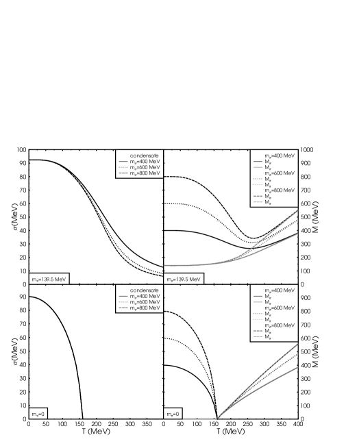
I start the discussion of the results with the chiral condensate $\sigma$ and the 4-momentum independent mass of the $\sigma$-meson and the pion, $M_{\sigma}$ and $M_{\pi}$, as defined in Eqs. (20) and (17). Note, that the 4-momentum independent mass $M_{\sigma}$ is generally not the physical (pole) mass of the $\sigma$-meson, because the pole of the $\sigma$-meson spectral density is additionally shifted by the 4-momentum dependent part of the selfenergy $[\mbox{Re}\,\Sigma(K,\sigma)]_{2}$, cf. Fig. 3.

In the upper row of Fig. 2 the results for the chiral condensate $\sigma$ (left column) and the 4-momentum independent mass for the pion and the $\sigma$-meson, $M_{\pi}$ and $M_{\sigma}$ (right column), are shown as functions of $T$ and $m_{\sigma}$, in the case of explicit chiral symmetry breaking. The results show the behaviour of a crossover transition. Neither the chiral condensate nor the 4-momentum independent mass of the scalar particle $M_{\sigma}$ become equal zero, even for high temperatures. Thus, $M_{\pi}$ and $M_{\sigma}$, become only approximatively degenerate for high temperatures. In the lower row of Fig. 2 the corresponding results for the chiral limit are presented. The results show the behaviour of a second-order phase transition, which agrees with the predictions made by Pisarski and Wilczek Pisarski and Wilczek (1984). The condensate $\sigma$ becomes equal zero at a critical temperature $T_{\chi}$, therefore $M_{\sigma}=M_{\pi}$ for $T\geq T_{\chi}$. The condensate (accordingly $T_{\chi}$) does not depend on the vacuum mass $m_{\sigma}$, which can be understood as a consequence of the condensate equation (10) in the chiral limit ($H=0$),

$$0=\mu^{2}+\frac{4\lambda}{N}\left[\sigma^{2}+N\,\int_{Q}\,{{\cal P}}(Q)\right].$$ (23)

For $m_{\pi}=0$ the integral can be performed analytically Lenaghan and Rischke (2000),

$$0=-\frac{m_{\sigma}^{2}}{2}+\frac{4\lambda}{N}\sigma^{2}+4\lambda\frac{T^{2}}{12}\Longrightarrow\sigma=\sqrt{f_{\pi}^{2}-\frac{T^{2}N}{12}}$$ (24)

[cf. Eq. (7)], and the critical temperature is given by $T_{\chi}=\sqrt{12/N}f_{\pi}\approx 160~{}{\rm MeV}$ for the $O(4)$ model, which agrees with the numerical results.

Figure 3: The 4-momentum dependent real part of the $\sigma$-meson selfenergy $[\mbox{Re}\,\Sigma]_{2}$, at a fixed momentum of $k=1$ GeV, for the case with explicit chiral symmetry breaking (full line) and the corresponding result for the chiral limit (dotted line) at a temperature of $T=120$ MeV.

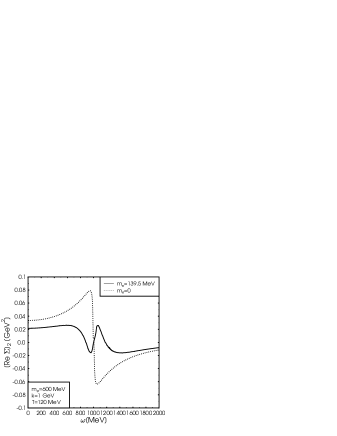
The 4-momentum dependent real part of the $\sigma$-meson selfenergy $[\mbox{Re}\,\Sigma]_{2}$ is shown in Fig. 3 at fixed momentum of $k=1$ GeV as a function of energy. It is larger in the chiral limit as in the case with explicit chiral symmetry breaking, because $[\mbox{Re}\,\Sigma]_{2}\sim\lambda^{2}\sim(m_{\sigma}^{2}-m_{\pi}^{2})^{2}$ is maximal for $m_{\pi}^{2}=0$. Note that $[\mbox{Re}\Sigma]_{2}$ is small compared to the (squared) 4-momentum independent mass of the $\sigma$-meson, shown in Fig. 2.

III.2 The decay width

After calculating the (4-momentum dependent) imaginary part of the $\sigma$-meson selfenergy (14), the decay width $\Gamma_{\sigma}$ is calculated at the quasiparticle energy: $\Gamma_{\sigma}(k)=\mbox{Im}\,\Sigma[\omega_{\sigma}(k),k;\sigma]/\omega_{\sigma}(k)$, where $\omega_{\sigma}(k)$ is given by the solution of $\omega_{\sigma}^{2}(k)-k^{2}-m_{\sigma}^{2}(\sigma)-\mbox{Re}\,\Sigma[\omega_{\sigma}(k),k;\sigma]=0$. The imaginary part of the selfenergy, and therefore the decay width, of the pion is of order $\sim 1/N$, and therefore neglected.

Figure 4: The decay width of the $\sigma$-meson $\Gamma_{\sigma}$, as a function of temperature $T$ and $\sigma$-meson vacuum mass $m_{\sigma}$, at momentum $k=1$ GeV, in the case with explicit chiral symmetry breaking (left) and in the chiral limit (right).

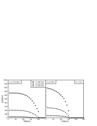
In Fig. 4 the decay width of the $\sigma$-meson $\Gamma_{\sigma}$ is shown as a function of temperature $T$. The qualitative behaviour is similar in all cases, but the decay width is larger in the chiral limit compared to the case with explicit chiral symmetry breaking, because $\mbox{Im}\,\Sigma\sim\lambda^{2}\sim(m_{\sigma}^{2}-m_{\pi}^{2})^{2}$ is maximal for $m_{\pi}^{2}=0$, cf. above discussion of $[\mbox{Re}\,\Sigma]_{2}$. The decay width is a strictly monotonic decreasing function with temperature, and becomes approximatively zero (equal zero) for temperatures larger than $\sim 200$ MeV ($T_{\chi}\approx 160$ MeV) in the case of explicit chiral symmetry breaking (the chiral limit). This is a consequence of the (partial) restoration of the chiral symmetry, the masses of the chiral partners become (approximatively) degenerate in mass, and therefore the phase space of the $\sigma\to 2\pi$ decay is squeezed. The dependence on the vacuum mass of the $\sigma$-meson is significant. The reason for this is that $\Gamma_{\sigma}\sim\mbox{Im}\,\Sigma\sim m_{\sigma}^{4}$, which agrees reasonably with the results, $\mbox{Im}\,\Sigma=1:3:16$ for $m_{\sigma}=400:600:800$ MeV.

Figure 5: The decay width of the $\sigma$-meson $\Gamma_{\sigma}$, in the improved Hartree (triangles) and in the improved Hartree-Fock (squares) approximation, as a function of temperature $T$, at momentum $k=1005$ MeV and $\sigma$-meson vacuum mass of $m_{\sigma}=600$ MeV, in the case with explicit chiral symmetry breaking.

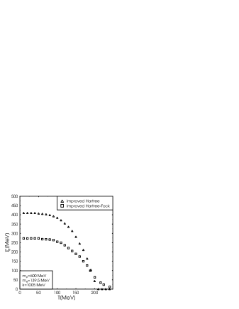
In Fig. 5 the decay width of the $\sigma$-meson in the improved Hartree (triangles) is compared with the improved Hartree-Fock Röder et al. (2005) (squares) approximation. The main difference stems from the combinatorial factor in front of the two-pion term ($\sim\int{\cal P}{\cal P}$) in the imaginary part of the selfenergy [cf. Eqs. (12a) with (14)]. A part of this contribution is of order $\sim 1/N$, and neglected in the Hartree approximation. Therefore, this factor is $2\cdot N=8$ in the improved Hartree, and $2\cdot(N-1)=6$ in the improved Hartree-Fock approximation, which would lead to a decay width of an factor $\approx 1.33$ larger in the improved Hartree approximation. The remaining difference, shown in the plot, comes from the $\sigma$-meson term ($\sim 3\cdot 3!\int{\cal S}{\cal S}$) in Eq. (14), which vanishes in the large-$N$ limit.

III.3 The spectral density

Finally, after solving the coupled condensate and Dyson-Schwinger equations selfconsistently, Eqs. (10) and (11), the spectral density of the $\sigma$-meson $\rho_{\sigma}$ is given in the chiral broken phase ($\sigma\neq 0$) by Eq. (18), and in the restored phase ($\sigma=0$) by Eq. (19).

Figure 6: The spectral density of the $\sigma$-meson $\rho_{\sigma}$, as a function of energy $\omega$, and $\sigma$-meson vacuum mass $m_{\sigma}$, at a momentum of $k=1$ GeV and a temperature of $T=100$ MeV, in the case with explicit chiral symmetry breaking (left) and the chiral limit (right).

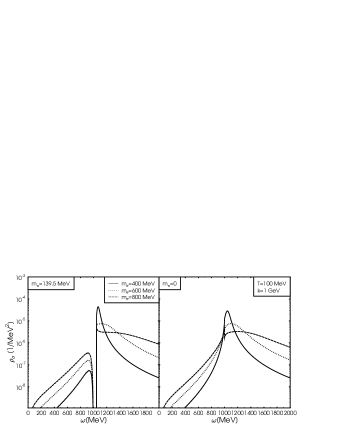
In Fig. 6 the spectral density is compared for all possible parameter sets (cf. table I) at a fixed momentum of $k=1$ GeV. The spectral density does not exhibit a pronounced peak at the quasiparticle energy $\omega_{\sigma}(k)$, because this energy is large enough for the decay into two pions. As discussed above, the decay width of this process is large and becomes even larger for increasing $m_{\sigma}$, as shown in the plot. A remarkable difference between the chiral limit (right) and the case with explicit chiral symmetry breaking (left) is, that $\rho_{\sigma}\approx 0$ around $\omega\approx 1$ GeV in the case with explicit symmetry breaking but not in the chiral limit. The reason is, that the threshold energy for $\sigma\rightarrow 2\pi$ is $\omega=2M_{\pi}$, and therefore zero in the chiral limit. For $\omega<k$ the $\sigma$-meson is Landau-damped.

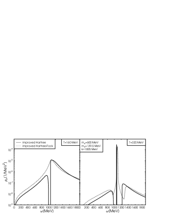
To illustrate the effects of neglecting terms of order $\sim 1/N$ in the improved Hartree approximation, I compare in Fig. 7 the results with the improved Hartree-Fock Röder et al. (2005) approximation, in the low-temperature regime at $T=160$ MeV (left), and in the high-temperature regime $T=320$ MeV (right). As show, the terms of order $\sim 1/N$ (included in the improved Hartree-Fock approximation) leads to a nonzero decay width of the pion, and therefore to a washed-out $\sigma$-meson spectral density. One aim of this work was to study the influence of the 4-momentum dependent real parts of the selfenergy. I found, that they does not lead to qualitative changes of the spectral density. To get an quantitative estimate, I consider the relative change between the spectral density with and without this real part, averaged over the energy-momentum grid, which is rather small, e.g. for the results shown in Fig. 7: $5.61\pm 2.90\%$ for $T=160~{}{\rm MeV}$, and $0.44\pm 0.01\%$ for $T=320~{}{\rm MeV}$.

IV Conclusions

In this paper I systematically improved the standard Hartree (or large-$N$) approximation of the $O(N)$ linear sigma model by taking into account, additionally to the double-bubble diagrams (shown in Figs. 1 a, b, c), the sunset diagrams (shown in Figs. 1 d, e) in the 2PI effective potential of the CJT formalism. This leads to 4-momentum dependent real and imaginary parts of the Dyson-Schwinger equations. I solve these and the equation of the condensate selfconsistently to get the decay width and the spectral density of the $\sigma$-meson, for the parameter sets summarized in table I.

First, I presented the results for the real parts of the Dyson-Schwinger, and the condensate equations. The 4-momentum independent parts, i.e., the 4-momentum independent masses and the chiral condensate exhibit a crossover transition in the case with explicit chiral symmetry breaking and a second order phase transition in the chiral limit, as predicted by Pisarski and Wilczek Pisarski and Wilczek (1984). The 4-momentum dependent real parts are small compared to the (squared) 4-momentum independent masses.

The decay width, presented in the second part of the results, show qualitatively the same behaviour in all cases. It is a strictly monotonic decreasing function with temperature, and becomes approximatively zero (equal zero) for temperatures larger than $\sim 200$ MeV ($T_{\chi}\approx 160$ MeV) in the case of explicit chiral symmetry breaking (the chiral limit). This is a consequence of the (partial) restoration of the chiral symmetry, the masses of the chiral partners becomes (approximatively) degenerate in mass, and therefore the phase space of the $\sigma\to 2\pi$ decay is squeezed. The dependence on the vacuum mass of the $\sigma$-meson is significant, because of $\Gamma_{\sigma}\sim\mbox{Im}\,\Sigma\sim m_{\sigma}^{4}$.

Finally, the behaviour of the decay width and the real parts are reflected in the spectral density. In the low-temperature regime, the spectral density is a very broad function in energy (and becomes even broader for larger vacuum mass $m_{\sigma}$) due to the $\sigma\to 2\pi$ decay and becomes more and more a delta function for increasing temperatures. The 4-momentum dependent real part of the selfenergy do not lead to qualitative changes.

The next step is to include also terms of order $\sim 1/N$, which would lead to a nonvanishing decay width of the pion and therefore to washed-out spectral densities. Other possible future projects are the inclusion of more degrees of freedom, for instance baryons Beckmann (2005), and vector mesons van Hees and Knoll (2000); Ruppert and Renk (2004); Strüber . The latter are of particular importance, since in-medium changes in the spectral properties of vector mesons are reflected in the dilepton spectrum Ruppert and Renk (2004) which, in turn, is experimentally observable in heavy-ion collisions at GSI-SIS, CERN-SPS and BNL-RHIC energies.

Figure 7: The spectral density of the $\sigma$-meson $\rho_{\sigma}$, as a function of energy $\omega$, at a momentum of $k=1$ GeV, and a vacuum $\sigma$-meson mass of $m_{\sigma}=600$MeV, in the case with explicit chiral symmetry breaking. The results are shown for the improved Hartree (full line) and the improved Hartree-Fock (dotted line) approximation at temperatures of $T=160$ MeV (left), and 320 MeV (right).

Appendix: The 4-momentum dependent parts of the selfenergy

In this section I derive the equations for the 4-momentum dependent imaginary and real part of the selfenergy (stemming from the sunset diagram). As discussed in Röder et al. (2005) this diagram can be expressed as a function of the spectral density $\rho_{\pi}$ in the imaginary time formalism

$$\Sigma(-i\omega_{m},k) = \left(\frac{4\lambda\sigma}{N}\right)^{2}\frac{2N}{(2\pi)^{4}}\frac{1}{k}\int_{-\infty}^{\infty}d\omega_{1}\,d\omega_{2}\frac{1+f(\omega_{1})+f(\omega_{2})}{i\omega_{m}+\omega_{1}+\omega_{2}}$$ (25)

$$\times \int_{0}^{\infty}dq_{1}\,q_{1}\,dq_{2}\,q_{2}\;\Theta\left(|q_{1}-q_{2}|\leq k\leq q_{1}+q_{2}\right)\rho_{\pi}(\omega_{1},q_{1})\rho_{\pi}(\omega_{2},q_{2}),$$

where $f(\omega)=1/[\exp(\omega/T)-1]$ is the Bose-Einstein distribution function, and $\omega_{m}=2\pi mT$ are the Matsubara frequencies. To extract the imaginary part, one uses the Dirac identity, $\mbox{Im}1/(x+i\epsilon)=-\pi\delta(x)$, and analytic continuation, $-i\omega_{m}\rightarrow\omega+i\epsilon$, for the retarded self-energy,

$$\mbox{Im}\,\Sigma(\omega,k) = \left(\frac{4\lambda\sigma}{N}\right)^{2}\frac{N}{2(2\pi)^{3}}\frac{1}{k}\int_{-\infty}^{\infty}d\omega_{1}\,d\omega_{2}[1+f(\omega_{1})+f(\omega_{2})]\,\delta(\omega-\omega_{1}-\omega_{2})$$ (26)

$$\times \int_{0}^{\infty}dq_{1}\,q_{1}\,dq_{2}\,q_{2}\;\Theta\left(|q_{1}-q_{2}|\leq k\leq q_{1}+q_{2}\right)\rho_{\pi}(\omega_{1},q_{1})\rho_{\pi}(\omega_{2},q_{2}).$$

As discussed in Sec. II in the improved Hartree approximation of the $O(N)$ model the spectral density of the pion is just a delta function (16),

$$\mbox{Im}\,\Sigma(\omega,k) = \left(\frac{4\lambda\sigma}{N}\right)^{2}\frac{N}{8\pi}\frac{1}{k}\int_{-\infty}^{\infty}d\omega_{1}\,d\omega_{2}[1+f(\omega_{1})+f(\omega_{2})]\,\delta(\omega-\omega_{1}-\omega_{2})$$ (27)

$$\times \int_{0}^{\infty}dq_{1}\,q_{1}\,dq_{2}\,q_{2}\;\Theta\left(|q_{1}-q_{2}|\leq k\leq q_{1}+q_{2}\right)[\omega_{\pi}(q_{1})\omega_{\pi}(q_{2})]^{-1}$$

$$\times \left\{\delta[\omega_{1}-\omega_{\pi}(q_{1})]\,\delta[\omega_{2}-\omega_{\pi}(q_{2})]+\delta[\omega_{1}+\omega_{\pi}(q_{1})]\,\delta[\omega_{2}+\omega_{\pi}(q_{2})]\right.$$

$$-\left.\delta[\omega_{1}-\omega_{\pi}(q_{1})]\,\delta[\omega_{2}+\omega_{\pi}(q_{2})]-\delta[\omega_{1}+\omega_{\pi}(q_{1})]\,\delta[\omega_{2}-\omega_{\pi}(q_{2})]\right\}\;,$$

where $\omega_{\pi}(q)=\sqrt{q^{2}+M_{\pi}^{2}}$ is the quasiparticle energy of the pion. To simplify this expression one uses the $\delta(\omega-\omega_{1}-\omega_{2})$ function to carry out the $\omega_{2}$-integration,

$$\mbox{Im}\,\Sigma(\omega,k) = \left(\frac{4\lambda\sigma}{N}\right)^{2}\frac{N}{8\pi}\frac{1}{k}\int_{-\infty}^{\infty}d\omega_{1}[1+f(\omega_{1})+f(\omega-\omega_{1})]$$ (28)

$$\times \int_{0}^{\infty}dq_{1}\,q_{1}\,dq_{2}\,q_{2}\;\Theta\left(|q_{1}-q_{2}|\leq k\leq q_{1}+q_{2}\right)[\omega_{\pi}(q_{1})\omega_{\pi}(q_{2})]^{-1}$$

$$\times \left\{\delta[\omega_{1}-\omega_{\pi}(q_{1})]\,\delta[\omega-\omega_{1}-\omega_{\pi}(q_{2})]+\delta[\omega_{1}+\omega_{\pi}(q_{1})]\,\delta[\omega-\omega_{1}+\omega_{\pi}(q_{2})]\right.$$

$$-\left.\delta[\omega_{1}-\omega_{\pi}(q_{1})]\,\delta[\omega-\omega_{1}+\omega_{\pi}(q_{2})]-\delta[\omega_{1}+\omega_{\pi}(q_{1})]\,\delta[\omega-\omega_{1}-\omega_{\pi}(q_{2})]\right\}\;,$$

and the $\omega_{1}$-integration with the help of the $\delta[\omega_{1}\pm\omega_{\pi}(q_{1})]$-functions

$$\mbox{Im}\,\Sigma(\omega,k) = \left(\frac{4\lambda\sigma}{N}\right)^{2}\frac{N}{8\pi}\frac{1}{k}\int_{0}^{\infty}dq_{1}\,q_{1}\,dq_{2}\,q_{2}\;\Theta\left(|q_{1}-q_{2}|\leq k\leq q_{1}+q_{2}\right)[\omega_{\pi}(q_{1})\omega_{\pi}(q_{2})]^{-1}$$ (29)

$$\times (\,\{1+f[\omega_{\pi}(q_{1})]+f[\omega-\omega_{\pi}(q_{1})]\}\,\delta[\omega-\omega_{\pi}(q_{1})-\omega_{\pi}(q_{2})]$$

$$+\{1+f[-\omega_{\pi}(q_{1})]+f[\omega+\omega_{\pi}(q_{1})]\}\,\delta[\omega+\omega_{\pi}(q_{1})+\omega_{\pi}(q_{2})]$$

$$-\{1+f[\omega_{\pi}(q_{1})]+f[\omega-\omega_{\pi}(q_{1})]\}\,\delta[\omega-\omega_{\pi}(q_{1})+\omega_{\pi}(q_{2})]$$

$$-\{1+f[-\omega_{\pi}(q_{1})]+f[\omega+\omega_{\pi}(q_{1})]\}\,\delta[\omega+\omega_{\pi}(q_{1})-\omega_{\pi}(q_{2})])\;.$$

The $\delta[\omega+\omega_{\pi}(q_{1})+\omega_{\pi}(q_{2})]$ function has no support, because $\omega>0$ and $\omega_{\pi}(q)>0$. Note that evaluating the $\delta[\omega-\omega_{\pi}(q_{1})+\omega_{\pi}(q_{2})]$ and the $\delta[\omega+\omega_{\pi}(q_{1})-\omega_{\pi}(q_{2})]$ function, the latter two terms cancels each other. The remaining delta function can be transformed to a delta function in momentum-space, $\delta[\omega-\omega_{\pi}(q_{1})-\omega_{\pi}(q_{2})]=|\omega_{\pi}(q_{0})/q_{0}|\,[\delta(q_{1}-q_{0})+\delta(q_{1}+q_{0})]$ where $q_{0}\equiv\sqrt{[\omega-\omega_{\pi}(q_{2})]^{2}-M_{\pi}^{2}}$, is the root of the argument of the delta function. Note that in Eq. (29) $q_{1}>0$ and therefore there is no support of the $\delta(q_{1}+q_{0})$ function. Carrying out the the $q_{1}$-integration, using $\omega-\omega_{\pi}(q_{0})=\omega_{\pi}(q_{1})$, and relabelling $q\equiv q_{2}$, one gets

$$\mbox{Im}\,\Sigma(\omega,k) = \left(\frac{4\lambda\sigma}{N}\right)^{2}\frac{N}{8\pi}\frac{1}{k}\int_{0}^{\infty}\,dq\;q\,[\omega_{\pi}(q)]^{-1}\Theta\left(|q_{0}-q|\leq k\leq q_{0}+q\right)$$ (30)

$$\times \{1+f[\omega_{\pi}(q_{0})]+f[\omega_{\pi}(q)]\}.$$

To calculate the limit $k\to 0$, best one starts with Eq. (29), uses the transformation $1+f[\omega_{\pi}(q_{1})]+f[\omega-\omega_{\pi}(q_{1})]=[1-\exp(-\omega/T)]\{1+f[\omega_{\pi}(q_{1})]\}\{1+f[\omega-\omega_{\pi}(q_{1})]\}$, the identity

$$\lim_{k\to 0}\frac{\Theta\left(|q_{1}-q_{2}|\leq k\leq q_{1}+q_{2}\right)}{k}=2\,\delta(q_{1}-q_{2})$$ (31)

(to perform the $q_{1}$-integration), and relabels $q\equiv q_{2}$, to get

$$\mbox{Im}\,\Sigma(\omega,0) = \left(\frac{4\lambda\sigma}{N}\right)^{2}\frac{N}{4\pi}\left[1-\exp\left(-\frac{\omega}{T}\right)\right]\int_{0}^{\infty}dq\,q^{2}\,\delta[\omega-2\omega_{\pi}(q)][\omega^{2}_{\pi}(q)]^{-1}$$ (32)

$$\times \{1+f[\omega_{\pi}(q)]\}\{1+f[\omega-\omega_{\pi}(q)]\}.$$

As discussed in detail in appendix E of Ref. Rischke (1998), this expression can be calculated analytically, using the Spence integral,

$$\mbox{Im}\,\Sigma(\omega,0)=\left(\frac{4\lambda\sigma}{N}\right)^{2}N\frac{1}{8\pi}\sqrt{1-\frac{4M_{\pi}^{2}}{\omega^{2}}}\coth\frac{\omega}{4T}\;.$$ (33)

Note that in Rischke (1998) the calculation is performed for the special case $\omega=m_{\sigma}$, but this can be generalised without further problems.

To calculate the real part of Eq.(25), one has to integrate over the principal value of $1/(\omega_{1}+\omega_{2}-\omega)$, denoted by $\mbox{P}\int\dots$,

$$[\mbox{Re}\,\Sigma(\omega,k)]_{2} = \left(\frac{4\lambda\sigma}{N}\right)^{2}\frac{2N}{(2\pi)^{4}}\frac{1}{k}\mbox{P}\int_{-\infty}^{\infty}d\omega_{1}\,d\omega_{2}\frac{1+f(\omega_{1})+f(\omega_{2})}{\omega_{1}+\omega_{2}-\omega}$$ (34)

$$\times \int_{0}^{\infty}dq_{1}\,q_{1}\,dq_{2}\,q_{2}\;\Theta\left(|q_{1}-q_{2}|\leq k\leq q_{1}+q_{2}\right)\rho_{\pi}(\omega_{1},q_{1})\rho_{\pi}(\omega_{2},q_{2}).$$

Again, one first uses the fact that the spectral density of the pion is just a delta function, which can be used to perform the $\omega_{1}$- and the $\omega_{2}$-integration. Using trivial renormalisation, i.e., neglecting the divergent parts leads to

$$[\mbox{Re}\,\Sigma(\omega,k)]_{2} = \left(\frac{4\lambda\sigma}{N}\right)^{2}\frac{N}{8\pi^{2}}\frac{1}{k}\mbox{P}\int_{0}^{\infty}dq_{1}\,q_{1}\,dq_{2}\,q_{2}\;\Theta\left(|q_{1}-q_{2}|\leq k\leq q_{1}+q_{2}\right)[\omega_{\pi}(q_{1})\omega_{\pi}(q_{2})]^{-1}$$ (35)

$$\times \left\{\frac{f[\omega_{\pi}(q_{1})]+f[\omega_{\pi}(q_{2})]}{\omega_{\pi}(q_{1})+\omega_{\pi}(q_{2})-\omega}+\frac{f[\omega_{\pi}(q_{1})]+f[\omega_{\pi}(q_{2})]}{\omega_{\pi}(q_{1})+\omega_{\pi}(q_{2})+\omega}\right.$$

$$\left.+\frac{-f[\omega_{\pi}(q_{1})]+f[\omega_{\pi}(q_{2})]}{\omega_{\pi}(q_{1})-\omega_{\pi}(q_{2})-\omega}+\frac{-f[\omega_{\pi}(q_{1})]+f[\omega_{\pi}(q_{2})]}{\omega_{\pi}(q_{1})-\omega_{\pi}(q_{2})+\omega}\right\}\;.$$

To evaluate the principal value numerically, in an appropriate way, one performs the following steps. First one introduces a new variable $x\equiv\omega_{\pi}(q_{1})$ and transforms the $q_{1}$-integration to an $x$-integration, with $dq_{1}=\omega_{\pi}(q_{1})/q_{1}dx$, and $q_{1}=\sqrt{x^{2}-M_{\pi}^{2}}\equiv q^{*}$. Relabelling $q\equiv q_{2}$ leads to

$$[\mbox{Re}\,\Sigma(\omega,k)]_{2} = \left(\frac{4\lambda\sigma}{N}\right)^{2}\frac{N}{8\pi^{2}}\frac{1}{k}\mbox{P}\int_{0}^{\infty}\,dq\,q\,[\omega_{\pi}(q)]^{-1}dx\,\Theta\;\left(|q^{*}-q|\leq k\leq q^{*}+q\right)$$

$$\times \left\{\frac{f(x)+f[\omega_{\pi}(q)]}{x+\omega_{\pi}(q)-\omega}+\frac{f(x)+f[\omega_{\pi}(q)]}{x+\omega_{\pi}(q)+\omega}\right.\left.+\frac{-f(x)+f[\omega_{\pi}(q)]}{x-\omega_{\pi}(q)-\omega}+\frac{-f(x)+f[\omega_{\pi}(q)]}{x-\omega_{\pi}(q)+\omega}\right\}.$$

Second one transforms the $x$-integration to a sum over $x_{i}$, and uses the mean value theorem to put the terms with the distribution functions in front of the integrals

$$[\mbox{Re}\,\Sigma(\omega,k)]_{2} = \left(\frac{4\lambda\sigma}{N}\right)^{2}\frac{N}{8\pi^{2}}\frac{1}{k}\mbox{P}\int_{0}^{\infty}\,dq\,q\,[\omega_{\pi}(q)]^{-1}\sum_{i}\Theta\;\left(|q^{*}-q|\leq k\leq q^{*}+q\right)$$ (37)

$$\times \left(\{f(\hat{x})+f[\omega_{\pi}(q)]\}\int_{x_{i}}^{x_{i+1}}dx\frac{1}{x+\omega_{\pi}(q)-\omega}\right.$$

$$+\{f(\hat{x})+f[\omega_{\pi}(q)]\}\int_{x_{i}}^{x_{i+1}}dx\frac{1}{x+\omega_{\pi}(q)+\omega}$$

$$+\{-f(\hat{x})+f[\omega_{\pi}(q)]\}\int_{x_{i}}^{x_{i+1}}dx\frac{1}{x-\omega_{\pi}(q)-\omega}$$

$$+\left.\{-f(\hat{x})+f[\omega_{\pi}(q)]\}\int_{x_{i}}^{x_{i+1}}dx\frac{1}{x-\omega_{\pi}(q)+\omega}\right),$$

where $x_{i}\leq\hat{x}\leq x_{i+1}$, and $q^{*}\equiv\sqrt{\hat{x}-M_{\pi}^{2}}$. Finally, the $x$-integrals can be performed analytically,

$$[\mbox{Re}\,\Sigma(\omega,k)]_{2} = \left(\frac{4\lambda\sigma}{N}\right)^{2}\frac{N}{8\pi^{2}}\frac{1}{k}\int_{0}^{\infty}\,dq\,q\,[\omega_{\pi}(q)]^{-1}\sum_{i}\Theta\;\left(|q^{*}-q|\leq k\leq q^{*}+q\right)$$ (38)

$$\times \left(\{f(\hat{x})+f[\omega_{\pi}(q)]\}\ln\left|\frac{[\omega_{\pi}(q)+x_{i+1}]^{2}-\omega^{2}}{[\omega_{\pi}(q)+x_{i}]^{2}-\omega^{2}}\right|\right.$$

$$+\left.\{-f(\hat{x})+f[\omega_{\pi}(q)]\}\ln\left|\frac{[\omega_{\pi}(q)-x_{i+1}]^{2}-\omega^{2}}{[\omega_{\pi}(q)-x_{i}]^{2}-\omega^{2}}\right|\right).$$

In the limit $k\to 0$, using Eq. (31), the $q$-integration can be carried out,

$$[\mbox{Re}\,\Sigma(\omega,0)]_{2} = \left(\frac{4\lambda\sigma}{N}\right)^{2}\frac{N}{4\pi^{2}}\sum_{i}\,q^{*}\,[\omega_{\pi}(q^{*})]^{-1}$$ (39)

$$\times \left(\{f(\hat{x})+f[\omega_{\pi}(q^{*})]\}\ln\left|\frac{[\omega_{\pi}(q^{*})+x_{i+1}]^{2}-\omega^{2}}{[\omega_{\pi}(q^{*})+x_{i}]^{2}-\omega^{2}}\right|\right.$$

$$+\left.\{-f(\hat{x})+f[\omega_{\pi}(q^{*})]\}\ln\left|\frac{[\omega_{\pi}(q^{*})-x_{i+1}]^{2}-\omega^{2}}{[\omega_{\pi}(q^{*})-x_{i}]^{2}-\omega^{2}}\right|\right).$$

References

- Amelino-Camelia (1997) G. Amelino-Camelia, Phys. Lett. B407, 268 (1997), eprint hep-ph/9702403.
- Roh and Matsui (1998) H.-S. Roh and T. Matsui, Eur. Phys. J. A1, 205 (1998), eprint nucl-th/9611050.
- Bochkarev and Kapusta (1996) A. Bochkarev and J. I. Kapusta, Phys. Rev. D54, 4066 (1996), eprint hep-ph/9602405.
- Baym and Grinstein (1977) G. Baym and G. Grinstein, Phys. Rev. D15, 2897 (1977).
- Gell-Mann and Levy (1960) M. Gell-Mann and M. Levy, Nuovo Cim. 16, 705 (1960).
- Lenaghan and Rischke (2000) J. T. Lenaghan and D. H. Rischke, J. Phys. G26, 431 (2000), eprint [http://arXiv.org/abs]nucl-th/9901049.
- Petropoulos (1999) N. Petropoulos, J. Phys. G25, 2225 (1999), eprint [http://arXiv.org/abs]hep-ph/9807331.
- Dumitru et al. (2004) A. Dumitru, D. Röder, and J. Ruppert, Phys. Rev. D70, 074001 (2004), eprint hep-ph/0311119.
- Baacke and Michalski (2003) J. Baacke and S. Michalski, Phys. Rev. D67, 085006 (2003), eprint hep-ph/0210060.
- Patkos et al. (2002) A. Patkos, Z. Szep, and P. Szepfalusy, Phys. Lett. B537, 77 (2002), eprint hep-ph/0202261.
- Röder et al. (2003) D. Röder, J. Ruppert, and D. H. Rischke, Phys. Rev. D68, 016003 (2003), eprint nucl-th/0301085.
- Chiku and Hatsuda (1998) S. Chiku and T. Hatsuda, Phys. Rev. D58, 076001 (1998), eprint hep-ph/9803226.
- Andersen et al. (2004) J. O. Andersen, D. Boer, and H. J. Warringa, Phys. Rev. D70, 116007 (2004), eprint hep-ph/0408033.
- Mocsy et al. (2004) A. Mocsy, I. N. Mishustin, and P. J. Ellis, Phys. Rev. C70, 015204 (2004), eprint nucl-th/0402070.
- Cabrera et al. (2005) D. Cabrera, E. Oset, and M. J. Vicente Vacas, Phys. Rev. C72, 025207 (2005), eprint nucl-th/0503014.
- Vicente Vacas and Oset (2002) M. J. Vicente Vacas and E. Oset (2002), eprint nucl-th/0204055.
- Scavenius et al. (2001) O. Scavenius, A. Mocsy, I. N. Mishustin, and D. H. Rischke, Phys. Rev. C64, 045202 (2001), eprint nucl-th/0007030.
- Dolan and Jackiw (1974) L. Dolan and R. Jackiw, Phys. Rev. D9, 3320 (1974).
- Braaten and Pisarski (1990a) E. Braaten and R. D. Pisarski, Phys. Rev. Lett. 64, 1338 (1990a).
- Braaten and Pisarski (1990b) E. Braaten and R. D. Pisarski, Nucl. Phys. B337, 569 (1990b).
- Cornwall et al. (1974) J. M. Cornwall, R. Jackiw, and E. Tomboulis, Phys. Rev. D10, 2428 (1974).
- Luttinger and Ward (1960) J. M. Luttinger and J. C. Ward, Phys. Rev. 118, 1417 (1960).
- Baym (1962) G. Baym, Phys. Rev. 127, 1391 (1962).
- Röder et al. (2005) D. Röder, J. Ruppert, and D. H. Rischke (2005), eprint hep-ph/0503042.
- Eidelman et al. (2004) S. Eidelman, K. Hayes, K. Olive, M. Aguilar-Benitez, C. Amsler, D. Asner, K. Babu, R. Barnett, J. Beringer, P. Burchat, et al., Physics Letters B 592, 1+ (2004), URL http://pdg.lbl.gov.
- Le Bellac (2000) M. Le Bellac, Thermal Field theory (Cambridge University Press, 2000).
- Weldon (1983) H. A. Weldon, Phys. Rev. D28, 2007 (1983).
- Pisarski and Wilczek (1984) R. D. Pisarski and F. Wilczek, Phys. Rev. D29, 338 (1984).
- Beckmann (2005) C. Beckmann, Acta Phys. Hung. A22, 215 (2005).
- van Hees and Knoll (2000) H. van Hees and J. Knoll, Nucl. Phys. A683, 369 (2000), eprint [http://arXiv.org/abs]hep-ph/0007070.
- Ruppert and Renk (2004) J. Ruppert and T. Renk (2004), eprint nucl-th/0412047.
- (32) S. Strüber, (in preparation).
- Rischke (1998) D. H. Rischke, Phys. Rev. C58, 2331 (1998), eprint nucl-th/9806045.