IPPP/05/60   DCPT/05/118
Probing Unquenching Effects in the Gluon Polarisation in Light Mesons

Abstract

We introduce an extension to the ladder truncated Bethe–Salpeter equation for mesons and the rainbow truncated quark Schwinger–Dyson equations which includes quark-loop corrections to the gluon propagator. This truncation scheme obeys the axialvector Ward-Takahashi identity relating the quark self-energy and the Bethe–Salpeter kernel. Two different approximations to the Yang-Mills sector are used as input: the first is a sophisticated truncation of the full Yang-Mills Schwinger–Dyson equations, the second is a phenomenologically motivated form. We find that the spectra and decay constants of pseudoscalar and vector mesons are overall described well for either approach. Meson mass results for charge eigenstate vector and pseudoscalar meson masses are compared to lattice data. The effects of unquenching the system are small but not negligible.

I Introduction

One of the longstanding problems of the theory of the strong interaction, Quantum Chromodynamics [QCD], is the description of hadronic bound states and resonances from first principles. Ironically it is perhaps the most interesting aspect of QCD, the phenomenon of confinement, that greatly hinders the development of our understanding of the experimental hadron spectrum: the individual components of these hadrons, dressed quarks and gluons, do not appear as physically observable states in nature. Thus, in order to study the internal structure of hadrons one has to resort to theoretical frameworks that connect the fundamental fields of the theory with phenomenology while preserving the basic low energy properties of QCD: confinement and dynamical chiral symmetry breaking.

Lattice simulations are not entirely satisfactory in this respect. They provide values for the global properties of hadrons (masses, decay widths etc.,) which, when compared with experiment, reassure us that QCD is indeed the theory of strong interactions. But they may not be capable to provide enough information on the internal structure of these hadrons, which is vital for our understanding of the dynamical aspects of low energy QCD. An alternative field theoretical and relativistic method which is well suited to provide this information is the Schwinger–Dyson and Bethe-Salpeter formalism (see, for example, iz ; Alkofer:2000wg ; Roberts:2000aa ; Maris:2003vk for a contemporary introduction to the topic). In principle this approach allows one to derive meson properties directly from the fundamental building blocks of the field theory, the Green’s functions.

From a technical point of view, lattice simulations and the Green’s functions approach are complementary to each other in several respects. Lattice calculations are ab initio and thus contain all effects from quantum fluctuations. However, they are limited to a comparably small momentum range and suffer from finite volume effects in the infrared. Furthermore the implementation of realistic quark masses turns out to be extremely involved from the viewpoint of computational times and is probably not feasible in the near future. Schwinger–Dyson equations [SDEs] can be solved analytically in the infrared and provide numerical solutions for a large momentum range. Together with the corresponding Bethe–Salpeter framework all aspects of chiral symmetry are respected such that the properties and effects of light quarks can be determined systematically with reasonable effort. On the other hand, in order to obtain closed systems of equations one has to introduce suitable approximations of higher order n-point functions. These truncations have to be controlled by comparing results from the SDE-approach to corresponding lattice data. In turn, the Schwinger–Dyson approach provides important information in momentum and quark mass regions that are not (yet) accessible on the lattice.

One of the most important recent developments in the Bethe–Salpeter formalism is the realisation that the chiral symmetry breaking pattern of the pseudoscalar meson sector is governed by the relationship between the quark propagator SDE and the Bethe–Salpeter kernel supplied by the axialvector Ward-Takahashi identity Maris:1997hd . This observation has led to the development of phenomenologically motivated models to describe the light pseudoscalar and vector meson properties Maris:1999nt ; Alkofer:2002bp . These models are constructed using the simplest truncation scheme (the rainbow/ladder truncation) known to satisfy the axialvector Ward-Takahashi identity. The Yang-Mills sector of QCD is replaced by an ansatz for the effective interaction between the quarks which is sufficiently strong to induce spontaneous chiral symmetry breaking and associated dynamical quark mass generation. This provided a robust starting point to determine various aspects of the light pseudoscalar and vector mesons like charge form factors Maris:2000sk ; Volmer:2000ek , electroweak and strong decays Maris:2001am ; Jarecke:2002xd and electroweak transitions Maris:2002mz ; Ji:2001pj . Exploratory studies go beyond the rainbow-ladder truncation by including corrections to the quark-gluon vertex Bender:2002as ; Bhagwat:2004hn ; Watson:2004kd .

Despite their phenomenological success, these models are unsatisfactory in an important respect. It is not clear, to what extent the structure of the Yang-Mills sector of QCD is represented by the ansätze used for the effective quark-gluon interaction. Certainly, if one strives for a detailed understanding of the internal structure of mesons it is vital to investigate (rather than to model) the effects of the Yang-Mills sector on experimental observables much more explicitly. This is one of the two central aims of the present work. Based on previous studies Alkofer:2000wg ; Fischer:2002hn of the pure Yang-Mills sector, results for the quenched and unquenched ghost, gluon and quark propagators from their coupled set of Schwinger–Dyson equations (SDEs) have been obtained in Ref. Fischer:2003rp . Here we extend this setup to include the corresponding Bethe-Salpeter equations and determine light pseudoscalar and vector meson observables. The effective interaction of the quark and gluons is hereby explicitly resolved in terms of the dressed gluon propagator and the dressed quark-gluon vertex.

The second aim of this work is to quantify a class of unquenching effects in meson observables. In general, ’unquenching’ means the inclusion of quark loops to the various correlation functions that enter the expressions for the quark self-energy and Bethe–Salpeter kernel. A previous study of unquenching focused on the mechanism for meson decay Watson:2004jq where a single quark loop could be incorporated into the truncation scheme, retaining the crucial property of obeying the axialvector Ward-Takahashi identity. However, there exists another viable improvement to the basic Bethe–Salpeter truncation scheme and this involves the unquenching of the input Yang-Mills interaction form with an infinite series of increasing numbers of quark loops. This is the second main issue of the present work.

The paper is organised as follows: In section II we detail our treatment of the ghost, gluon and quark propagators. We investigate unquenching effects due to quark loops in these quantities in two different setups. On the one hand we explicitly solve the coupled set of (unquenched) Schwinger–Dyson equations for the ghost, gluon and quark propagators employing ansätze for the various vertex functions. On the other hand we investigate the same effects employing a model for the quenched Yang-Mills sector of QCD, which we effectively unquench by adding a quark-loop to the model gluon propagator. The results in both setups are used as input for our calculation of pseudoscalar and vector meson properties, detailed in section III. Numerical results and conclusions are reported in sections IV and V. Various technical aspects are discussed in the appendices. Throughout the various stages of our calculation we will compare our results from the SDE/BSE approach with those from recent lattice simulations. Finally, it is worth noting that whenever we refer to unquenching in the present work we only refer to unquenching effects due to the presence of quark loops in the gluon-SDE. Certainly, as already mentioned above, unquenching the full theory involves other important effects like meson decays which are beyond the scope of this study.

II Unquenched propagators

To start with, we describe in some detail the two calculational schemes that we use to determine the effects of quark loops on the propagators of QCD. The first scheme employs the full set of coupled unquenched SDEs for the ghost, gluon and quark propagators together with appropriate ansätze for the ghost-gluon, the three-gluon and the quark-gluon vertex. We use a slightly modified truncation compared to the one used in Ref. Fischer:2003rp . The second scheme employs a model for the quark-gluon-interaction, which has been shown in Ref. Alkofer:2002bp to be well suited for phenomenological investigations. In both schemes we take unquenching effects in the gluon polarisation explicitly into account.

II.1 Propagators from the quark, gluon and ghost Schwinger–Dyson equations

For the purpose of our investigation we work in Landau gauge QCD, with the gauge fixing performed by the familiar Faddeev-Popov method. The resulting determinant is conveniently represented by a pair of Grassmann-fields, the Faddeev-Popov ghosts. The two-point functions of Landau gauge QCD, the ghost, gluon and quark propagators can be generically written as

$$D_{G}^{ab}(p) = -\frac{G(p^{2})}{p^{2}}\delta^{ab}\,,$$ (1)

$$D_{\mu\nu}^{ab}(p) = \left(\delta_{\mu\nu}-\frac{p_{\mu}p_{\nu}}{p^{2}}\right)\frac{Z(p^{2})}{p^{2}}\delta^{ab}\,,$$ (2)

$$S_{i}(p) = \frac{1}{-ip\hskip-5.0pt/\,A_{i}(p^{2})+B_{i}(p^{2})}=\frac{Z_{f}^{i}(p^{2})}{-ip\hskip-5.0pt/+M_{i}(p^{2})}\,.$$ (3)

Here $G(p^{2})$ denotes the ghost dressing function, $Z(p^{2})$ the gluon dressing function, and $A_{i}(p^{2})$ and $B_{i}(p^{2})$ are the vector and scalar quark self energy of the quark flavors $i\in\{u,d,s\}$. In a somewhat different notation, $M_{i}(p^{2})=B_{i}(p^{2})/A_{i}(p^{2})$ is the quark mass function, whereas $Z_{f}^{i}(p^{2})=1/A_{i}(p^{2})$ is called the quark wave function. The corresponding bare tree level propagators, $D_{G}^{0}(p)$, $D^{0}_{\mu\nu}(p)$ and $S_{i}^{0}(p)$ are given by $Z\equiv G\equiv Z_{f}\equiv 1$ and $M_{i}(p^{2})=m_{i}$, where the $m_{i}$ are the respective renormalised quark masses in the Lagrangian of QCD. The color factors of objects in the adjoint representation are given explicitly, whereas the color factors of objects in the fundamental representation are treated implicitly.

The propagators (1), (2) and (3) satisfy the coupled set of renormalised Schwinger–Dyson -equations,

$${[D^{af}(p)]^{-1}_{\mu\nu}} = Z_{3}[D^{0,af}(p)]^{-1}_{\mu\nu}-\tilde{Z_{1}}\int\,\,\,\raisebox{-1.72218pt}{\large$\bar{}$}\!\!d\,{k}\,\>\widetilde{\Gamma}^{0,abc}_{\mu}(p,k)\>D_{G}^{bd}(p-k)\>\widetilde{\Gamma}_{\nu}^{def}(k,p)D_{G}^{ce}(k)$$ (4)

$$-Z_{1}\,\frac{1}{2}\,\int\,\,\,\raisebox{-1.72218pt}{\large$\bar{}$}\!\!d\,{k}\,\>\Gamma^{0,abc}_{\mu\rho\sigma}(p,k)\>D_{\rho\rho^{\prime}}^{bd}(p-k)\>\Gamma_{\rho^{\prime}\nu\sigma^{\prime}}^{def}(k,p)D_{\sigma\sigma^{\prime}}^{ce}(k)$$

$$-Z_{1F}\,\frac{1}{2}\,\sum_{i=u,d,s}\int\,\,\,\raisebox{-1.72218pt}{\large$\bar{}$}\!\!d\,{k}\,\>\>\mbox{Tr}\left\{\Gamma_{\mu}^{0,a}\,S_{i}(k)\,\Gamma_{\nu}^{a}(k,p)\,S_{i}(p-k)\right\}\ +\ \left(\dots\right),$$

$${[D^{af}_{G}(p)]^{-1}} = \tilde{Z_{3}}[D_{G}^{0,ab}(p)]^{-1}-\tilde{Z_{1}}\,\int\,\,\,\raisebox{-1.72218pt}{\large$\bar{}$}\!\!d\,{k}\,\>\widetilde{\Gamma}^{0,abc}_{\mu}(p,k)\>D_{\mu\nu}^{bd}(p-k)\>\widetilde{\Gamma}_{\nu}^{def}(k,p)D_{G}^{ce}(k)\;,\hskip 42.67912pt$$ (5)

$$S_{i}^{-1}(p) = Z_{2}\,[S_{i}^{0}(p)]^{-1}-Z_{1F}\,\int\,\,\,\raisebox{-1.72218pt}{\large$\bar{}$}\!\!d\,{k}\,\,\Gamma_{\mu}^{0,a}(p,k)\,S_{i}(k)\,\Gamma_{\nu}^{b}(k,p)\,D_{\mu\nu}^{ab}(p-k)\,,$$ (6)

which are given diagrammatically in Fig. 1. Here $\,\,\,\raisebox{-1.72218pt}{\large$\bar{}$}\!\!d\,{k}\,$ is an abbreviation of $d^{4}k/(2\pi)^{4}$. The sum in the quark-loop runs over the light quark flavors and the trace is over color and Dirac indices. The ghost-gluon vertex is denoted by $\widetilde{\Gamma}_{\nu}^{abc}(k,p)$, the three-gluon vertex is given by $\Gamma_{\rho\nu\sigma}^{abc}(k,p)$ and ${\Gamma}_{\nu}^{a}(k,p)$ is the quark-gluon vertex. The corresponding bare quantities have an additional superscript $0$. The ellipsis in the gluon-SDE represents two-loop diagrams containing the four-gluon-vertex. The gluon tadpole diagram vanishes in the process of renormalisation and is therefore omitted from the start. The SDEs (4), (5) and (6) are renormalised and therefore finite and independent of the ultraviolet regulator $\Lambda$. The definitions of the renormalisation constants $Z_{i}$ are given in appendix A together with the corresponding relations between unrenormalised and renormalised dressing functions.

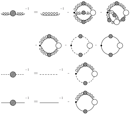
Figure 1: A diagrammatical representation of the coupled system of ghost, gluon and quark Schwinger–Dyson equations. Filled blobs denote dressed propagators and empty circles denote dressed proper vertex functions.

The quenched system of ghost- and gluon-SDEs, Eqs. (5) and (4) without the quark loop, and the quark-SDE (6) have been investigated separately in a series of publications vonSmekal:1997is ; Atkinson:1997tu ; Alkofer:2000wg ; Watson:2001yv ; Zwanziger:2001kw ; Lerche:2002ep ; Fischer:2002hn ; Zwanziger:2003cf ; Alkofer:2004it ; Maris:1997tm ; Maris:1997hd ; Bloch:2002eq ; Bhagwat:2003vw ; Maris:2003vk . Results for the unquenched system, including the back-coupling of the quarks onto the Yang-Mills sector, have been reported in Fischer:2003rp . In the following we shortly summarise some results, which are important for the present work.

The infrared behaviour of the ghost and gluon propagators can be determined self-consistently from the ghost-SDE and the ghost-loop in the gluon-SDE alone. This so called ghost-dominance of Yang-Mills theory in the infrared has been conjectured in Ref. vonSmekal:1997is , lead to the formulation of an infrared effective theory based solely on the Faddeev-Popov determinant Zwanziger:2003cf and has recently been shown to hold in a self-consistent scenario of solutions for general n-point functions Alkofer:2004it . In Landau gauge, such an analysis is based on the factorisation property of the ghost-gluon vertex, which entails that in the presence of one external scale this vertex cannot develop any nontrivial dressing (i.e. singularities or zeros) in the infrared Watson:2001yv ; Lerche:2002ep ; Taylor:ff . Based on this observation one finds simple power laws,

$$Z(p^{2})\sim(p^{2})^{2\kappa},\hskip 28.45274ptG(p^{2})\sim(p^{2})^{-\kappa},$$ (7)

for the gluon and ghost dressing function with exponents related to each other. The relations (7) can be determined from the ghost-SDE alone and are independent of any approximation of the ghost-gluon vertex, which is in agreement with the factorisation property. The exponent $\kappa$ is an irrational number and depends only slightly on the dressing of the ghost-gluon vertex Lerche:2002ep . With a bare vertex one obtains $\kappa=(93-\sqrt{1201})/98\approx 0.595$ Lerche:2002ep ; Zwanziger:2001kw . This result has been confirmed independently in studies of the exact renormalisation group equation Pawlowski:2003hq . Lattice simulations indicate that $\kappa\approx 0.5$ Leinweber:1998im ; Bowman:2004jm ; Gattnar:2004bf ; Oliveira:2004gy ; Sternbeck:2005tk , see however Fischer:2005ui for a discussion on systematic effects on $\kappa$ due to a compact manifold.

Probably the most interesting consequence of the power laws (7) is the corresponding fixed point of the running coupling $\alpha(p^{2})$ in the infrared. A nonperturbative definition of this coupling can be derived from the ghost-gluon-vertex vonSmekal:1997is ,

$$\alpha(p^{2})=\frac{g^{2}}{4\pi}G^{2}(p^{2})Z(p^{2}).$$ (8)

No vertex function appears in this definition; a fact that can be traced back to the ultraviolet finiteness of the ghost-gluon vertex in Landau gauge. Note that the right hand side is a renormalisation group invariant, i.e. $\alpha(p^{2})$ does not depend on the renormalisation point. From the power laws (7) one finds that the coupling has a fixed point in the infrared, given by Lerche:2002ep

$$\alpha(0)=\frac{4\pi}{6N_{c}}\frac{\Gamma(3-2\kappa)\Gamma(3+\kappa)\Gamma(1+\kappa)}{\Gamma^{2}(2-\kappa)\Gamma(2\kappa)}\approx 2.972\\$$ (9)

for the gauge group SU(3) and a bare ghost-gluon vertex. Interestingly enough, both, the values of the exponent $\kappa$ and the fixed point $\alpha(0)$ can be shown to be independent of the gauge parameter in a class of gauges that interpolate between Landau and Coulomb gauge Fischer:2005qe .

Numerical solutions for the ghost and gluon propagator for general momenta have been obtained in refs. Fischer:2002hn ; Fischer:2003rp . In the infrared these solutions agree with the infrared asymptotic behaviour of Eq.(7), whereas in the ultraviolet they reproduce corresponding results from resummed perturbation theory. The employed approximation scheme for the ghost-gluon-vertex, the three-gluon-vertex and the four-gluon-vertex is detailed in Fischer:2002hn . For the convenience of the reader we summarise the basic assumptions of this truncation in appendix B. Here we discuss our truncation of the quark-gluon-vertex in more detail, as this vertex provides the crucial link between the Yang-Mills SDEs, the quark-SDE and the Bethe–Salpeter equation describing mesons as bound states of quarks and antiquarks.

The structure of the quark-gluon-vertex has been the focus of some interest in the last years. It is well known, that the leading $\gamma_{\mu}$-part of the vertex provides sufficient structure to the quark-gluon interaction to describe a range of properties of the pseudoscalar and vector mesons well (see Maris:2003vk and references therein). On the other hand it is also well known by now, that further tensor structure in the vertex, in particular a scalar part, is mandatory to describe other meson channels. Such corrections to the vertex have been investigated on a semiperturbative level in several works Bender:1996bb ; Bender:2002as ; Bhagwat:2004hn ; Watson:2004kd ; Bhagwat:2004kj ; Fischer:2004ym and comparisons with first lattice results Skullerud:2002ge ; Skullerud:2003qu are encouraging (although the error bars from such simulations are still quite large). Unfortunately, the numerical complexity of the present investigation is such that we are not able to include such corrections. Instead, we will adopt the strategy of Ref. Fischer:2003rp and employ an ansatz for the nonperurbative dressing of the $\gamma_{\mu}$-part of the vertex such that important constraints like multiplicative renormalisability and a correct perturbative limit of the vertex are satisfied.

With $k$ denoting the gluon momentum and $p,q$ the two respective quark momenta, two possible ansätze for the vector part of the quark-gluon-vertex are

$$\Gamma_{\nu}^{a}(q,p) = igT^{a}\,\gamma_{\nu}\,\frac{G^{2}(k^{2})}{Z_{1F}}\,A(k^{2}),$$

$$\Gamma_{\nu}^{a}(q,p) = igT^{a}\,\gamma_{\nu}\,\frac{G(p^{2})G(q^{2})}{Z_{1F}}\,\frac{A(p^{2})+A(q^{2})}{2}.$$ (10)

The presence of the vector quark self energy $A(k^{2})$ in these expressions is enforced by the Slavnov-Taylor identity for the quark-gluon vertex (given in appendix A), which also accounts for one of the two ghost factors. The second ghost factor leads to a perturbative behaviour of the vertex, which produces the correct perturbative anomalous dimensions of the ghost, gluon and quark propagators in the ultraviolet momentum regime, provided the momentum arguments of the dressing functions are chosen in an appropriate way. As discussed in detail in Ref. Fischer:2003rp , the first version of arguments, is necessary in the quark-SDE, whereas the second version has to be chosen in the quark loop of the gluon-SDE to reproduce the respective correct perturbative limits of these equations. Via the renormalisation properties of the contributing dressing functions and the vertex renormalisation constant $Z_{1F}$ this ansatz has the correct dependence on the renormalisation scale $\mu^{2}$ in agreement with the renormalisation group. Furthermore note that both versions of the vertex have the correct properties under charge conjugation. The price to be paid with this construction is its cutoff-dependence via $Z_{1F}$. Thus these ansätze do not have all properties of well defined renormalised Green’s functions, but have to be regarded as effective constructions, which only make sense in connection with the quark- and gluon-SDE. If inserted into these equations, the ansätze lead to properly renormalised, cutoff-independent ghost, gluon and quark propagators.

Together with the truncations for the other vertices, specified in appendix B, we end up with the following set of coupled, nonlinear integral equations for the ghost, gluon and quark propagators

$$\frac{1}{G(p^{2})} = \tilde{Z}_{3}-g^{2}N_{c}\int\,\,\,\raisebox{-1.72218pt}{\large$\bar{}$}\!\!d\,{k}\,\frac{K(p^{2},k^{2},q^{2})}{p^{2}k^{2}}G(k^{2})Z(q^{2})\;,$$ (11)

$$\frac{1}{Z(p^{2})} = {Z}_{3}+g^{2}\frac{N_{c}}{3}\int\,\,\,\raisebox{-1.72218pt}{\large$\bar{}$}\!\!d\,{k}\,\frac{M(p^{2},k^{2},q^{2})}{p^{2}k^{2}}G(k^{2})G(q^{2})+g^{2}\frac{N_{c}}{3}\int\,\,\,\raisebox{-1.72218pt}{\large$\bar{}$}\!\!d\,{k}\,\frac{Q(p^{2},k^{2},q^{2})}{p^{2}k^{2}}\frac{G(k^{2})^{(-2-6\delta)}}{Z(k^{2})^{3\delta}}\frac{G(q^{2})^{(-2-6\delta)}}{Z(q^{2})^{3\delta}}$$ (12)

$$-g^{2}\,Z_{2}\,\sum_{i=u,d,s}\int\,\,\,\raisebox{-1.72218pt}{\large$\bar{}$}\!\!d\,{k}\,\frac{G(k)}{k^{2}+M_{i}^{2}(k^{2})}\frac{G(q)}{q^{2}+M_{i}^{2}(q^{2})}\frac{A_{i}(k^{2})+A_{i}(q^{2})}{2A_{i}(k^{2})A_{i}(q^{2})}W(p^{2},k^{2},q^{2})\,,$$

$$B_{i}(p^{2}) = Z_{2}\>m_{i}+Z_{2}\,\frac{4}{3}\,\int\,\,\,\raisebox{-1.72218pt}{\large$\bar{}$}\!\!d\,{k}\,\frac{4\pi\alpha(q^{2})A_{u}(q^{2})}{q^{2}}\,\frac{3B_{i}(k^{2})}{k^{2}A_{i}^{2}(k^{2})+B_{i}^{2}(k^{2})}\,,$$ (13)

$$A_{i}(p^{2}) = Z_{2}+Z_{2}\,\frac{4}{3}\,\int\,\,\,\raisebox{-1.72218pt}{\large$\bar{}$}\!\!d\,{k}\,\frac{4\pi\alpha(q^{2})A_{u}(q^{2})}{q^{2}}\frac{A_{i}(k^{2})}{k^{2}A_{i}^{2}(k^{2})+B_{i}^{2}(k^{2})}\left(-\frac{q^{2}}{p^{2}}+\frac{p^{2}+k^{2}}{2p^{2}}+\frac{(p^{2}-k^{2})^{2}}{2\>q^{2}p^{2}}\right)\,,$$ (14)

where $\delta=-9N_{c}/(44N_{c}-8N_{f})$ is the one-loop anomalous dimension of the ghost propagator and $i\in\{u,d,s\}$. Note that with our choice (10) of the quark-gluon-vertex it is the running coupling $\alpha(q^{2})$ (cf. Eq.(8)) multiplied with the quark self energy $A_{u}(q^{2})$ that provides the interaction in the quark-SDEs. In order to allow the construction of a Bethe-Salpeter kernel in accordance with the axialvector Ward-Takahashi identity the interaction in the quark-SDEs has to be flavor independent and is therefore always chosen to contain the $A$-function of the lightest (up-)quark. The kernels ordered with respect to powers of $q^{2}=(p-k)^{2}$ have the form:

$$K(p^{2},k^{2},q^{2}) = \frac{1}{q^{4}}\left(-\frac{(p^{2}-k^{2})^{2}}{4}\right)+\frac{1}{q^{2}}\left(\frac{p^{2}+k^{2}}{2}\right)-\frac{1}{4}\,,$$

$$M(p^{2},k^{2},q^{2}) = \frac{1}{q^{2}}\left(-\frac{1}{4}p^{2}+\frac{k^{2}}{2}-\frac{1}{4}\frac{k^{4}}{p^{2}}\right)+\frac{1}{2}+\frac{1}{2}\frac{k^{2}}{p^{2}}-\frac{1}{4}\frac{q^{2}}{p^{2}}\,,$$

$$Q(p^{2},k^{2},q^{2}) = \frac{1}{q^{4}}\left(\frac{1}{8}\frac{p^{6}}{k^{2}}+p^{4}-\frac{9}{4}p^{2}k^{2}+k^{4}+\frac{1}{8}\frac{k^{6}}{p^{2}}\right)$$

$$+\frac{1}{q^{2}}\left(\frac{p^{4}}{k^{2}}-4p^{2}-4k^{2}+\frac{k^{4}}{p^{2}}\right)$$

$$-\left(\frac{9}{4}\frac{p^{2}}{k^{2}}+4+\frac{9}{4}\frac{k^{2}}{p^{2}}\right)+q^{2}\left(\frac{1}{p^{2}}+\frac{1}{k^{2}}\right)+q^{4}\frac{1}{8p^{2}k^{2}}$$

$$W(p^{2},k^{2},q^{2}) = \frac{q^{4}}{3p^{4}}+q^{2}\left(\frac{1}{3p^{2}}-\frac{2k^{2}}{3p^{4}}\right)-\frac{2}{3}+\frac{k^{2}}{3p^{2}}+\frac{k^{4}}{3q^{4}}\,.$$ (15)

The momentum subtracted versions of Eqs. (11)-(14) are employed in our numerical investigations. (An outline of the subtraction procedure is given in section IV.1.1.)

II.2 The phenomenological model

As a simpler (at least in some respects) alternative to the above described setup, we employ a model for the effective interaction between quarks and gluons, which has been developed in Alkofer:2002bp . This effective interaction $\Delta_{\mu\nu}^{ab}$ can be related to the combination of dressed gluon propagator and dressed $\gamma_{\mu}$-part of the quark-gluon vertex in the following way:

$$\Gamma_{\mu}^{0,a}(p,k)\,D_{\mu\nu}^{ab}(p-k)\,\Gamma_{\nu}^{b}(k,p)\hskip 14.22636pt\longrightarrow\hskip 14.22636pt\imath T^{a}\gamma_{\mu}\,g^{2}\Delta_{\mu\nu}^{ab}(p-k)\,\imath T^{b}\gamma_{\nu}$$ (16)

where both vertices are replaced by their tree-level counterparts ($\Gamma_{\mu}^{0,a}=\imath gT^{a}\gamma_{\mu}$). The central premise of phenomenologically constructing the effective interaction is that of integrated infrared strength – the interaction, when input into the quark self-energy integral, must be capable of generating sufficient amounts of dynamical chiral symmetry breaking [D$\chi$SB] in order to generate the experimentally observed hadronic mass spectra. One such construction is the quenched, Landau gauge form

$$g^{2}\Delta_{\mu\nu}^{0,ab}(p)=\delta^{ab}\,t_{\mu\nu}(p)\,4\pi^{2}\,d\,\frac{p^{2}}{\omega^{2}}\,\exp{\left(-\frac{p^{2}}{\omega^{2}}\right)}\,,$$ (17)

where $t_{\mu\nu}(p)$ is the transverse momentum projector. The parameters $d$ and $\omega$ are fitted by comparing the resultant pseudoscalar meson mass and leptonic decay constant to experiment. The parameter $\omega$, which sets the position of the maximum of the interaction, can be regarded as a length scale associated with the interaction, and $d$ relates to the overall magnitude. It turns out that the meson masses (and the pseudoscalar and vector leptonic decay constants) are largely independent of $\omega$ in the range $\omega\sim 0.2-0.7\mathrm{GeV}$. As an example $\omega=0.5\mathrm{GeV}$, $d=16\mathrm{GeV}^{-2}$ gives realistic results for the pseudoscalar and vector channels Alkofer:2002bp .

Figure 2: Schwinger–Dyson equations for the quark and gluon propagator under the truncation scheme of the phenomenological model. All vertices are tree-level. Blobs represent fully dressed propagators. The seed term of the gluon equation is dressed with the Gaussian form Eq. 17 (see text).

Clearly, by fitting to experiment, there is implicit information contained within such a phenomenological interaction about quark loops contained within the choice of parameters. However, the quark loops are at least from the viewpoint of truncated equations an additional degree of freedom. In the context of a full field theory (QCD here) such inclusions are self-consistently present as described in the previous subsection. In order to make such contributions also apparent in this phenomenological model we unquench the effective interaction by adding to the phenomenological Gaussian form a quark loop term which generates an infinite series of increasing numbers of quark loops. The quark-gluon vertex itself remains undressed. The truncated set of SDEs for this phenomenological model is shown in Fig. 2.

The equation for the unquenched effective interaction is

$$\Delta_{\mu\nu}^{ab}(p)=\Delta_{\mu\nu}^{0,ab}(p)-\,\Delta_{\mu\lambda}^{0,ac}(p)\,g^{2}\delta^{cd}\,t_{\lambda\rho}(p)\,p^{2}\,\Sigma(p^{2})\,\Delta_{\rho\nu}^{db}(p)$$ (18)

with

$$g^{2}\,\delta^{cd}\,t_{\lambda\rho}(p)\,p^{2}\,\Sigma(p^{2})=g^{2}\,\delta^{cd}\,t_{\lambda\rho}(p)\,p^{2}\,Z_{\Delta}+\int\,\,\,\raisebox{-1.72218pt}{\large$\bar{}$}\!\!d\,{k}\,\sum_{i=u,d,s}\,Tr\left[\imath gT^{c}\gamma_{\lambda}\,S^{i}(k)\,\imath gT^{d}\gamma_{\rho}\,S^{i}(k-p)\right]$$ (19)

where the sum runs over the light quark flavors and the trace is over color and Dirac indices. The prefactors in the definition of $\Sigma$ are such that $\Sigma$ is a dimensionless scalar function. The renormalisation constant $Z_{\Delta}$ is independent of the external momentum scale and has been introduced to cancel the UV divergence of the quark loop. One can see that the integral of the right-hand side in Eq. (19) is transverse with respect to momentum $p$ in exactly the same way as for the one-loop perturbative quark loop contribution to the gluon polarisation due to the presence of the tree-level vertices. Making the color and tensor structure of the effective interaction explicit with

$$\Delta_{\mu\nu}^{ab}(k)=\delta^{ab}t_{\mu\nu}(k)\Delta(k^{2})$$ (20)

and projecting out the scalar part $\Delta(k^{2})$ from Eqs. (18) and (19) (see section IV.1.1 for more discussion on the projection) we arrive at

$$\Delta(p^{2})=\frac{\Delta^{0}(p^{2})}{1+g^{2}\Delta^{0}(p^{2})p^{2}\Sigma(p^{2})}$$ (21)

with

$$\Sigma(p^{2})=Z_{\Delta}+\frac{4}{3}\,\int\,\,\,\raisebox{-1.72218pt}{\large$\bar{}$}\!\!d\,{k}\,\,\sum_{i=u,d,s}\,\frac{1}{k^{2}+M^{2}(k^{2})}\frac{1}{q^{2}+M^{2}(q^{2})}\frac{1}{A(k^{2})A(q^{2})}\left[\frac{k^{2}}{p^{2}}-4\frac{p\!\cdot\!k^{2}}{p^{4}}+3\frac{p\!\cdot\!k}{p^{2}}\right].$$ (22)

where the momentum $q=k-p$.

For the quark dressing functions $A(p^{2})$ and $B(p^{2})$ we obtain

$$B(p^{2}) = m+\frac{4}{3}\,\int\,\,\,\raisebox{-1.72218pt}{\large$\bar{}$}\!\!d\,{k}\,g^{2}\Delta(q^{2})\,\frac{3B(k^{2})}{k^{2}A^{2}(k^{2})+B^{2}(k^{2})}\,,$$ (23)

$$A(p^{2}) = 1+\frac{4}{3}\,\int\,\,\,\raisebox{-1.72218pt}{\large$\bar{}$}\!\!d\,{k}\,g^{2}\Delta(q^{2})\,\frac{A(k^{2})}{k^{2}A^{2}(k^{2})+B^{2}(k^{2})}\left(-\frac{q^{2}}{p^{2}}+\frac{p^{2}+k^{2}}{2p^{2}}+\frac{(p^{2}-k^{2})^{2}}{2\>q^{2}p^{2}}\right)\,,$$ (24)

Note that the renormalisation constants of the quark equations above have been set to unity since the effective interaction is exponentially damped in the UV and the subsequent integrals are convergent. These last four equations are used for our numerical investigations of unquenching effects in the phenomenological model. Further technical details concerning our method to solve these equations in the complex momentum plane (necessary to solve the Bethe–Salpeter equation in Euclidean space) are given in appendix C.

III The Bethe-Salpeter Equation

The homogeneous Bethe-Salpeter equation [BSE] for flavor non-singlet quark-antiquark mesons can be written

$$\Gamma_{\alpha\beta}^{ij}(p;P)=\int\,\,\,\raisebox{-1.72218pt}{\large$\bar{}$}\!\!d\,{k}\,K_{\alpha\beta;\delta\gamma}(p,k;P)\left[S^{i}(k_{+})\Gamma^{ij}(k;P)S^{j}(k_{-})\right]_{\gamma\delta}$$ (25)

where $K$ is the Bethe-Salpeter kernel, momenta $k_{+}=k+\xi P$ and $k_{-}=k+(\xi-1)P$ are such that the total momentum $P=k_{+}-k_{-}$ and $\xi=[0,1]$ is the momentum partitioning parameter reflecting the arbitrariness in the relative momenta of the quark-antiquark pair. The flavor content is expressed through the indices $i,j$ and for flavor non-singlet mesons the kernel can be written independently of flavor content. Greek indices ($\alpha\ldots$) refer to color and Dirac structure. The BSE is a parametric eigenvalue equation with discrete solutions $P^{2}=-M_{n}^{2}$ where $M_{n}$ is the mass of the resonance. The lowest mass solution corresponds to the physical ground state. Since $P^{2}$ is negative, the momenta $k_{\pm}$ are necessarily complex in Euclidean space and so the quark propagator functions must be evaluated with complex argument. This leads to technical issues that are dealt with in appendix C.

One of the defining characteristics of the light pseudoscalar meson sector is the pattern of chiral symmetry breaking and the identification of pions as the Goldstone bosons of the symmetry breaking. In the Bethe-Salpeter formalism this is associated with observance of the axialvector Ward-Takahashi identity [AXWTI] Maris:1997hd . The AXWTI serves to relate the quark self-energy and the Bethe-Salpeter kernel such that the pattern of chiral symmetry breaking in the pseudoscalar meson sector is guaranteed, independently of truncation or model details. In the flavor non-singlet channel and (for illustrative purposes) with equal mass quarks the AXWTI is

$$-\imath P_{\mu}\Gamma_{\mu}^{5}(p;P)=S^{-1}(p_{+})\gamma_{5}+\gamma_{5}S^{-1}(p_{-})-2m_{r}\Gamma^{5}(p;P)$$ (26)

where we have introduced the (color-singlet) axialvector and pseudoscalar vertices ($\Gamma_{\mu}^{5}$ and $\Gamma^{5}$, respectively) and $m_{r}$ is the renormalised quark mass. Defining

$$\Lambda(p;P)=-\imath P_{\mu}\Gamma_{\mu}^{5}(p;P)+2m_{r}\Gamma^{5}(p;P)$$ (27)

then the inhomogeneous Bethe–Salpeter integral equations for $\Gamma_{\mu}^{5}$ and $\Gamma^{5}$ can be combined to give (replacing the color and Dirac indices)

$$\Lambda_{\alpha\beta}(p;P)=\left[\imath Z_{2}\gamma_{5}\hbox to0.0pt{\hbox to7.80904pt{\hfil/\hfil}\hss}P+Z_{4}2m_{r}\gamma_{5}\right]_{\alpha\beta}+\int\,\,\,\raisebox{-1.72218pt}{\large$\bar{}$}\!\!d\,{k}\,K_{\alpha\beta;\delta\gamma}(p,k;P)\left[S(k_{+})\Lambda(k;P)S(k_{-})\right]_{\gamma\delta}.$$ (28)

Using the AXWTI to rewrite $\Lambda$ in terms of the quark propagator gives

$$\left[S^{-1}(p_{+})\gamma_{5}+\gamma_{5}S^{-1}(p_{-})\right]_{\alpha\beta}=\left[\imath Z_{2}\gamma_{5}\hbox to0.0pt{\hbox to7.80904pt{\hfil/\hfil}\hss}P+Z_{4}2m_{r}\gamma_{5}\right]_{\alpha\beta}+\int\,\,\,\raisebox{-1.72218pt}{\large$\bar{}$}\!\!d\,{k}\,K_{\alpha\beta;\delta\gamma}(p,k;P)\left[\gamma_{5}S(k_{-})+S(k_{+})\gamma_{5}\right]_{\gamma\delta}$$ (29)

and by writing the Schwinger–Dyson equation for the quark as

$$S^{-1}(p)=-Z_{2}\imath\hbox to0.0pt{\hbox to5.03125pt{\hfil/\hfil}\hss}p+Z_{4}m_{r}-\Sigma_{f}(p)$$ (30)

one can eliminate the inhomogeneous terms to get

$$\left[-\Sigma_{f}(p_{+})\gamma_{5}-\gamma_{5}\Sigma_{f}(p_{-})\right]_{\alpha\beta}=\int\,\,\,\raisebox{-1.72218pt}{\large$\bar{}$}\!\!d\,{k}\,K_{\alpha\beta;\delta\gamma}(p,k;P)\left[\gamma_{5}S(k_{-})+S(k_{+})\gamma_{5}\right]_{\gamma\delta},$$ (31)

thereby making the relationship between the quark self-energy $\Sigma_{f}$ and the Bethe–Salpeter kernel $K$ manifest.

For the truncation scheme given by the full-SDE set, in order to satisfy Eq. (31) we specify the truncated Bethe–Salpeter kernel to be:

$$K_{\alpha\beta;\delta\gamma}(p,k;P)\rightarrow\left[\Gamma_{\mu}^{0,a}(p_{+},k_{+})\right]_{\alpha\gamma}\left[\Gamma_{\nu}^{0,b}(k_{-},p_{-})\right]_{\delta\beta}\delta^{ab}t_{\mu\nu}(p-k)Z_{2}\frac{4\pi}{g^{2}}\frac{\alpha(p-k)A_{u}(p-k)}{(p-k)^{2}}\,,$$ (32)

where $A_{u}$ is the vector self energy of the up-quark regardless of the remaining flavor structure, which is left implicit. In the case of the phenomenological model, the kernel is nothing more than the standard dressed ladder truncation:

$$K_{\alpha\beta;\delta\gamma}(p,k;P)\rightarrow\left[\Gamma_{\mu}^{0,a}(p_{+},k_{+})\right]_{\alpha\gamma}\left[\Gamma_{\nu}^{0,b}(k_{-},p_{-})\right]_{\delta\beta}\delta^{ab}t_{\mu\nu}(p-k)\Delta(p-k).$$ (33)

Notice that the addition of the explicit quark loop in the expression for the interaction does not alter the structure of the kernel. Expanding out the various factors (retaining the flavor content), the Bethe–Salpeter equation for the two schemes are written as

$$\Gamma^{ij}(p;P)=-\frac{4}{3}Z_{2}\int\,\,\,\raisebox{-1.72218pt}{\large$\bar{}$}\!\!d\,{k}\,\frac{4\pi\alpha(p-k)A_{u}(p-k)}{(p-k)^{2}}t_{\mu\nu}(p-k)\gamma_{\mu}S^{i}(k_{+})\Gamma^{ij}(k;P)S^{j}(k_{-})\gamma_{\nu}$$ (34)

for the full SDE scheme and

$$\Gamma^{ij}(p;P)=-\frac{4}{3}\int\,\,\,\raisebox{-1.72218pt}{\large$\bar{}$}\!\!d\,{k}\,g^{2}\Delta(p-k)t_{\mu\nu}(p-k)\gamma_{\mu}S^{i}(k_{+})\Gamma^{ij}(k;P)S^{j}(k_{-})\gamma_{\nu}$$ (35)

for the phenomenological model.

Meson channels are specified by the quantum numbers $J^{PC}$ and flavor content. We assume isospin degeneracy ($m_{d}=m_{u}$) and consider only flavor non-singlet channels such that the flavor content of the meson can be generated in the BSE by supplying the appropriate quark propagators $S^{i}$ (henceforth we drop the flavor indices). The $J^{PC}$ quantum numbers are input into the BSE by specifying the Dirac and Lorentz decomposition of the bound-state vertices $\Gamma$ to have the relevant transformation properties. We shall be considering pseudoscalar ($0^{-+}$) and vector ($1^{--}$) mesons whose decompositions are:

$$\Gamma^{PS}(p;P) = \gamma_{5}\left[\Gamma_{0}(p;P)-\imath\hbox to0.0pt{\hbox to7.80904pt{\hfil/\hfil}\hss}P\Gamma_{1}(p;P)-\imath\hbox to0.0pt{\hbox to5.03125pt{\hfil/\hfil}\hss}p\Gamma_{2}(p;P)-\left[\hbox to0.0pt{\hbox to7.80904pt{\hfil/\hfil}\hss}P,\hbox to0.0pt{\hbox to5.03125pt{\hfil/\hfil}\hss}p\right]\Gamma_{3}(p;P)\right],$$ (36)

$$\Gamma_{\mu}^{V}(p;P) = \gamma_{\mu}^{T}\left[\imath\Gamma_{0}(p;P)+\hbox to0.0pt{\hbox to7.80904pt{\hfil/\hfil}\hss}P\Gamma_{1}(p;P)-\hbox to0.0pt{\hbox to5.03125pt{\hfil/\hfil}\hss}p\Gamma_{2}(p;P)+\imath\left[\hbox to0.0pt{\hbox to7.80904pt{\hfil/\hfil}\hss}P,\hbox to0.0pt{\hbox to5.03125pt{\hfil/\hfil}\hss}p\right]\Gamma_{3}(p;P)\right]$$ (37)

$$+p_{\mu}^{T}\left[\Gamma_{2}(p;P)+2\imath\hbox to0.0pt{\hbox to7.80904pt{\hfil/\hfil}\hss}P\Gamma_{3}(p;P)\right]$$

$$+p_{\mu}^{T}\left[\Gamma_{4}(p;P)+\imath\hbox to0.0pt{\hbox to7.80904pt{\hfil/\hfil}\hss}P\Gamma_{5}(p;P)-\imath\hbox to0.0pt{\hbox to5.03125pt{\hfil/\hfil}\hss}p\Gamma_{6}(p;P)+\left[\hbox to0.0pt{\hbox to7.80904pt{\hfil/\hfil}\hss}P,\hbox to0.0pt{\hbox to5.03125pt{\hfil/\hfil}\hss}p\right]\Gamma_{7}(p;P)\right],$$

where $\gamma_{\mu}^{T}$ and $p_{\mu}^{T}$ are transverse to $P_{\mu}$ (the on-shell vector meson is transverse to its total momentum $P$). The $\Gamma_{i}$ are scalar functions of $p^{2}$ and $p\!\cdot\!P$ ($P^{2}$ is on-shell for solutions of the BSE and therefore fixed). The charge conjugation properties of the decompositions above are such that when considering charge eigenstates, the $\Gamma_{i}$ are either odd or even under the interchange $p\!\cdot\!P\rightarrow-p\!\cdot\!P$. By projecting the BSE onto the covariant basis it becomes a coupled set of nonlinear integral equations for the $\Gamma_{i}$. The technical procedure of solving these equations is outlined in section IV.1.2.

The solution of the pseudoscalar BSE can be used to obtain the pion leptonic decay constant, $f_{\pi}$, which will prove useful in fitting parameters to observables. In order to calculate $f_{\pi}$ one must firstly normalise the BS vertex function $\Gamma$. The normalisation condition is derived by demanding that the residue of the pole in the four-point quark-antiquark Green’s function (from which the BSE is derived) be unity Tandy:1997qf ; Nakanishi:1969ph . For $\xi=1/2$ it reads

$$2P_{\mu}=3Tr_{d}\int\,\,\,\raisebox{-1.72218pt}{\large$\bar{}$}\!\!d\,{k}\,\left\{\overline{\Gamma}(k,-P)\frac{\partial S(k+P/2)}{\partial P_{\mu}}\Gamma(k,P)S(k-P/2)+\overline{\Gamma}(k,-P)S(k+P/2)\Gamma(k,P)\frac{\partial S(k-P/2)}{\partial P_{\mu}}\right\}_{P^{2}=-M^{2}}$$ (38)

where the trace is over Dirac matrices, both propagators describe $u$-quarks and the conjugate vertex function $\overline{\Gamma}$ is defined as

$$\overline{\Gamma}(p,-P)=C\Gamma^{T}(-p,-P)C^{-1}$$ (39)

with the charge conjugation matrix $C=-\gamma_{2}\gamma_{4}$. The leptonic decay constant characterising the pion coupling to the point axial field is subsequently given by Tandy:1997qf

$$f_{\pi}=\frac{3}{M^{2}}Tr_{d}\int\,\,\,\raisebox{-1.72218pt}{\large$\bar{}$}\!\!d\,{k}\,\Gamma(k,-P)S(k+P/2)\gamma_{5}\hbox to0.0pt{\hbox to7.80904pt{\hfil/\hfil}\hss}PS(k-P/2),$$ (40)

where again the trace is over Dirac matrices. Eq. (40) can also be applied to the kaon by inserting the corresponding quark propagators (with the apropriate normalisation).

IV Numerical Procedure and Results

IV.1 Technical details

IV.1.1 Renormalisation and subtraction procedure

To regularise the coupled system of ghost, gluon and quark SDEs we apply a MOM regularisation scheme vonSmekal:1997is ; Atkinson:1997tu ; Kizilersu:2001pd . If we write the equations (11), (12), (13) and (14) symbolically as

$$\frac{1}{G(p^{2})} = \tilde{Z}_{3}+\Pi_{ghost}(p^{2})\,,$$ (41)

$$\frac{1}{Z(p^{2})} = {Z}_{3}+\Pi_{glue}(p^{2})\,,$$ (42)

$$A(p^{2}) = Z_{2}+Z_{2}\,\Pi_{A}(p^{2})\,,$$ (43)

$$B(p^{2}) = Z_{4}\,m_{R}+Z_{2}\,\Pi_{B}(p^{2})\,,$$ (44)

where $m_{R}$ is the renormalised quark mass in the Lagrangian of the theory, this procedure yields

$$\frac{1}{G(p^{2})} = \frac{1}{G(\mu^{2})}+\Pi_{ghost}(p^{2})-\Pi_{ghost}(\mu^{2})\,,$$ (45)

$$\frac{1}{Z(p^{2})} = \frac{1}{Z(\mu^{2})}+\Pi_{glue}(p^{2})-\Pi_{glue}(\mu^{2})\,,$$ (46)

$$\frac{1}{A(p^{2})} = 1-\frac{1}{A(p^{2})}\Pi_{A}(p^{2})+\Pi_{A}(\mu^{2})\,,$$ (47)

$$B(p^{2}) = B(\mu^{2})+\frac{A(\mu^{2})}{1+\Pi_{A}(\mu^{2})}\,\left(\Pi_{B}(p^{2})-\Pi_{B}(\mu^{2})\right)\,,$$ (48)

where $\mu^{2}$ is a suitable renormalisation point. The a priori unknown renormalisation constants $Z_{3}$, $\tilde{Z}_{3}$ and $Z_{2}$ drop out and instead one specifies normalisation conditions for $G(\mu^{2})$, $Z(\mu^{2})$ and $A(\mu^{2})$. For a given renormalised coupling $g$ the Slavnov-Taylor identity

$$1=\widetilde{Z}_{1}=Z_{g}\>\widetilde{Z}_{3}\>Z_{3}^{1/2}.$$ (49)

enforces that one cannot choose the normalisation conditions for $G(\mu^{2})$ and $Z(\mu^{2})$ separately, but only for the product $Z(\mu^{2})\,G^{2}(\mu^{2})$, see Ref. vonSmekal:1997is . Multiplicative renormalisability implies that the dressing functions for different choices of $\mu$ are trivially related to each other by factors of the renormalisation constants. Note that the coupling $\alpha(p^{2})=\alpha(\mu^{2})G^{2}(p^{2})Z(p^{2})$ and the quark mass function $M(p^{2})=B(p^{2})/A(p^{2})$ are independent of the renormalisation point.

A further complication is the appearance of spurious quadratic divergencies in the gluon-SDE, which are not eliminated by the MOM procedure. In principle, quadratic divergencies can be avoided by contracting the right hand side of the gluon-SDE with the Brown-Pennington projector $R_{\mu\nu}(p)=\delta_{\mu\nu}-4\frac{p_{\mu}p_{\nu}}{p^{2}}$ Brown:1988bm ; Brown:1988bn . However, using this technique one picks up spurious longitudinal contributions from the right hand side of the gluon-SDE, which affect the value of $\kappa$ in the infrared power laws of the ghost and gluon dressing function, Eqs. (7) Lerche:2002ep ; Fischer:2002hn . We therefore employ an alternative procedure, which is well known in the context of exact renormalisation group equations Pawlowski:2003hq ; Ellwanger:1996wy . After contracting the right hand side of the gluon-SDE with the transverse projector, leading to Eq. (12), quadratic divergencies show up as terms proportional to $\Lambda^{2}/p^{2}$, where $\Lambda$ is the UV-cutoff. In the infrared, such terms can be identified unambiguously by fitting the right hand side to the form $a/p^{2}+b/(p^{2})^{2\kappa}$. The coefficient $a$ then measures all contributions from quadratic divergencies and is subtracted from the right hand side at each step of the numerical iteration procedure. Together with the MOM-scheme described above this procedure ensures that all renormalised dressing functions are independent of the regularisation scale.

The situation is somewhat simpler for the phenomenological model, specified in section II.2. The projection of the quark loop contribution to the interaction Eq. (19) can be carried out using the Brown-Pennington projector to eliminate quadratic divergences without further complication. Also, the form of the effective interaction Eq. (21) with the Gaussian term $\Delta^{0}(p^{2})$ alters the picture. $\Delta^{0}(p^{2})$ (and hence $\Delta(p^{2})$) vanishes exponentially in the UV, leaving the integrals for Eq. (24) and Eq. (23) UV convergent. The remaining integral for $\Sigma(p^{2})$ does though require regularisation and renormalisation since the quark functions do reduce to their tree-level values in the UV, producing a logarithmic divergence. Also here we use a subtractive scheme and define the renormalised dressing function $\overline{\Sigma}(p^{2})$ to be

$$\overline{\Sigma}(p^{2})=\Sigma(p^{2})-\Sigma({\mu^{2}})$$ (50)

such that $\overline{\Sigma}(p^{2}=\mu^{2})=0$ for some spacelike renormalisation scale $\mu$. We then take as our interaction

$$\Delta(p^{2})=\frac{\Delta^{0}(p^{2})}{1+g^{2}\Delta^{0}(p^{2})\,p^{2}\,\overline{\Sigma}(p^{2})}.$$ (51)

In what follows, we drop the overbar on $\Sigma$ and the subtraction is implicitly assumed though not written explicitly for notational convenience. The renormalisation scale $\mu$ is in principle a free parameter of the model. However, since we are studying light mesons with an associated hadronic scale of $\sim 1\mathrm{GeV}$ we expect $\mu$ to be in this region. It turns out that there is only a slight dependence of the overall results on $\mu$, reflecting the approximate observance of renormalisation scale invariance (c.f. appendix D). Throughout the main body of the paper we use the single value $\mu=1\mathrm{GeV}$.

There is one major distinction between the full SDE set and the phenomenological model and this concerns the role of the quark mass $m_{R}$. In the full set of SDEs, the renormalisation of the quark mass and its subsequent running with momentum scales allows one to compare the current quark mass with the perturbative quark mass. In the case of the phenomenological model however, the quark mass is nothing more than a parameter of the model and cannot be directly compared to any other quantity.

IV.1.2 Solving the Bethe-Salpeter equation

Projecting the BSE, Eq. 25 onto the covariant basis $\Gamma_{i}$ (for pseudoscalar and vector mesons given via the decompositions Eqs. 36 and 37 respectively) it becomes a coupled set of nonlinear integral equations. To solve this set the $\Gamma_{i}$ are approximated by a Chebyshev expansion in the angular variable $z=p\!\cdot\!P/\sqrt{p^{2}P^{2}}$,

$$\Gamma_{i}(p^{2},z;P^{2})=\sum_{k=0}^{N_{ch}-1}\imath^{k}T_{k}(z)\Gamma_{i}^{k}(p^{2};P^{2}).$$ (52)

Since the $T_{k}$ form an orthonormal set one can further project the equations onto this basis. In the case of charge eigenstate mesons, one can extract an explicit factor $p\!\cdot\!P$ from the odd $\Gamma_{i}$ and then use only the even $T_{k}$. The meson mass solution to the system of coupled equations in the $\Gamma_{i}^{k}$ is then found in one of two equivalent ways. The first is to introduce a fictitious linear eigenvalue $\lambda(M)$ so that the original BSE reads

$$\lambda(M)\Gamma_{\alpha\beta}(p;P)=\int\,\,\,\raisebox{-1.72218pt}{\large$\bar{}$}\!\!d\,{k}\,K_{\alpha\beta;\delta\gamma}(p,k;P)\left[S(k_{+})\Gamma(k;P)(k_{-})\right]_{\gamma\delta}$$ (53)

with $P^{2}=-M^{2}$ and vary the mass until $\lambda(M=M_{n})=1$ (the physical ground state corresponds to the largest real eigenvalue). The second method is to recognise that after decomposition, the final integral over the radial momentum must be discretized giving rise to a matrix equation $\Gamma_{i}^{k}(p_{j}^{2};P^{2})=K_{ii^{\prime}}^{kk^{\prime}}(p_{j}^{2},p_{j^{\prime}}^{2};P^{2})\Gamma_{i^{\prime}}^{k^{\prime}}(p_{j^{\prime}}^{2};P^{2})$ whose solution is the highest (physical ground state mass) $P^{2}=-M^{2}$ for which $\mbox{Det}(1-K)=0$.

In principle, a truncation of the Chebyshev expansion destroys the Poincaré covariance of the results, expressed through the invariance of the mass solution $M^{2}$ with the momentum sharing parameter $\xi$. However, the expansion quickly converges such that the numerical results are explicitly stable with varying $\xi$ Alkofer:2002bp . In this work we take $\xi=1/2$ and $N_{ch}=4(6)$ for the pseudoscalar (vector) meson channels.

IV.2 Numerical Results for the Propagator Functions

     

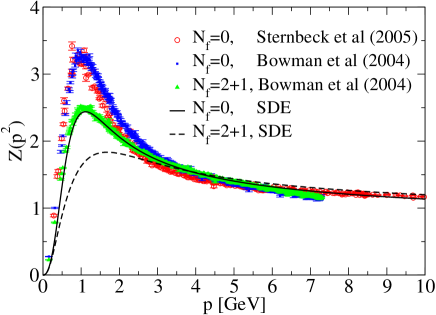
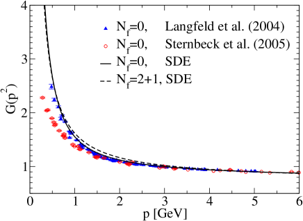
Figure 3: Comparison of the quenched and unquenched ghost and gluon dressing functions with recent lattice data Sternbeck:2005tk ; Bowman:2004jm ; Gattnar:2004bf . The sea-quark masses are $m_{u/d}\simeq 16\mbox{MeV},m_{s}\simeq 79\mbox{MeV}$ in the lattice simulations and $m_{u/d}\simeq 3.9\mbox{MeV},m_{s}\simeq 84\mbox{MeV}$ in the SDE-approach, c.f. table 2.

Our results for the (un)quenched ghost and gluon dressing functions from the full set of SDEs are displayed in figure 3. In the infrared, the numerical SDE-results reproduce the analytical power laws, Eqs.(7). (This can be seen explicitly on a log-log-plot, displayed e.g. in Ref. Fischer:2002hn ). In the ultraviolet they reproduce the correct one-loop running of resummed perturbation theory, with anomalous dimensions $\gamma=\frac{-13N_{c}+4N_{f}}{22N_{c}-4N_{f}}$ and $\delta=\frac{-9N_{c}}{44N_{c}-8N_{f}}$ for the gluon and ghost dressing functions. Compared to the results of recent lattice calculations Sternbeck:2005tk ; Bowman:2004jm ; Gattnar:2004bf we find good agreement for large and small momenta. In the intermediate momentum region one clearly sees unquenching effects in the gluon dressing function. In this momentum region the system has enough energy to create quark-antiquark pairs from the vacuum. The screening effect from these pairs, first seen in Ref.Fischer:2003rp , drives the gluon dressing function closer to its perturbative form, i.e. the bump in the dressing functions becomes smaller. This effect is pronounced in both, the SDE and the lattice results. The overall difference in the size of the gluon bump between the two approaches indicates that the (neglected) gluon-two-loop diagrams in the gluon-SDE have an influence in this momentum region. Moreover, adding additional tensor structure to the quark-gluon vertex changes the magnitude of the unquenching effects slightly, as can be seen by comparison with Fig.1 in Ref. Fischer:2004wf . In general, however, we expect that the inclusion of these contributions (in future work) will not change any of the conclusions drawn in this paper.

In comparing the quenched and unquenched interactions of the full SDE set and the phenomenological model, the situation is complicated by the presence of non-trivial quark masses. As pointed out previously, in the phenomenological model the quark masses are no more than parameters to be fitted to experimental results for meson observables (see next subsection for details). They cannot be compared directly to those of either the full SDE set or experiment. In addition, for both cases, the back reaction of the unquenching term induces changes to the fitted quark masses which further obscures the comparison. Therefore, to start the discussion we restrict for now to the chiral limit where a more unambiguous comparison can be made. Using the spacelike chiral quark propagator alone there are two quantities that can be compared in the quenched and unquenched truncations – the vacuum chiral quark condensate $<\overline{q}q>^{0}$ and the quark mass function at zero momentum, $M(0)$. The condensate is the order parameter for dynamical chiral symmetry breaking and at a renormalisation scale $\mu$ is defined as (see for example Ref. Langfeld:2003ye for a discussion on this topic)

$$<\overline{q}q>^{0}(\mu)=-\lim_{\Lambda\rightarrow\infty}Z_{4}(\mu,\Lambda)N_{c}Tr_{d}\int\,\,\,\raisebox{-1.72218pt}{\large$\bar{}$}\!\!d\,{k}\,S_{0}(k)$$ (54)

where $\Lambda$ is the regularisation scale, $S_{0}$ is the chiral limit of the quark propagator and the trace is over Dirac matrices. In the full set of SDEs we determine the (un)quenched condensate from the chiral quark propagator renormalised at a large scale $\mu^{2}$ and subsequently evolve the value down to $\mu=2\mathrm{GeV}$ employing one-loop scaling. For the phenomenological model, where $Z_{4}=1$, the condensate depends only indirectly on $\mu$ via the unquenching effects. In both approaches the unquenching effects on the quark-gluon interaction are calculated with physical sea quark configurations (see the next subsection for details of the fitting procedure and parameter values).

Our results for $<\overline{q}q>^{0}$ and $M(0)$ are presented in table 1. In the full SDE-setup with the quark-gluon vertex (10) we find a very slight enhancement of the condensate once quark-loops are taken into account. An even smaller effect has been found in Ref. Fischer:2003rp , where different approximations of the vertex have been investigated. These results together indicate that the condensate is almost constant for $N_{f}\leq 3$. Since the condensate is an order parameter for D$\chi$SB it is expected to change rapidly at the vicinity of the chiral phase transition. We conclude therefore that the critical number of flavors for the chiral transition of QCD at zero temperature is much larger than $N_{f}=3$. This agrees well with the recently estimated value $N_{f}^{c}=10.0\pm 0.4$ in the framework of exact renormalisation group equations Gies:2005as and expectations from perturbation theory. For the quark mass at zero momentum we note a reduction of $\sim 10\%$ due to quark-loop effects in both the full SDE and the phenomenological frameworks. A similar reduction has been found in Ref. Fischer:2003rp for a range of different truncations of the quark-gluon vertex. We therefore believe this effect to be model independent. Recent lattice simulations using staggered quarks confirm this result Bowman:2005vx .

Table 1: The chiral condensate and the chiral quark mass function at $p^{2}=0$ in the full-SDE setup and in the phenomenological model. The unquenching effects are calculated with physical sea-quarks, see tab. 2 for the corresponding values of the quark masses and interaction parameters.

	$-(<\overline{q}q>^{0})^{1/3}$ ($\mathrm{MeV}$)	$M_{ch}(p^{2}=0)$ ($\mathrm{MeV}$)
Model:
$N_{f}=0$	244	366
$N_{f}=2+1$	243	332
full SDE:
$N_{f}=0$	266	416
$N_{f}=2+1$	271	388

Next we compare the effective interaction of the phenomenological model, $g^{2}\Delta(p^{2})\,p^{2}/4\pi$, to the interaction of the full-SDE setup, $\alpha(p^{2})\,A(p^{2})$, at finite quark masses. The parameters of the two schemes are fixed to reproduce the physical pion and kaon observables (see the next subsection for details of the fitting procedure and parameter values). From the plot in Fig. 4 one notes drastic differences. The interaction of the full-SDE setup stretches from the deep infrared to the ultraviolet, where the perturbative one-loop running is reproduced. In the infrared the interaction is not vanishing due to the fixed point behaviour of the running coupling, Eq. (8), multiplied with a finite value of $A(0)$. The effective interaction of the phenomenological model, however, is localised at intermediate momenta. Despite the clear differences, both interactions produce similar qualitative effects in meson observables as will be seen in later sections. This is a validation of the assertion that the simplest $q\bar{q}$ meson states are dominated by the pattern of dynamical chiral symmetry breaking which arises from the integrated strength of the interaction and are not largely affected by the detailed structure of the interaction itself.

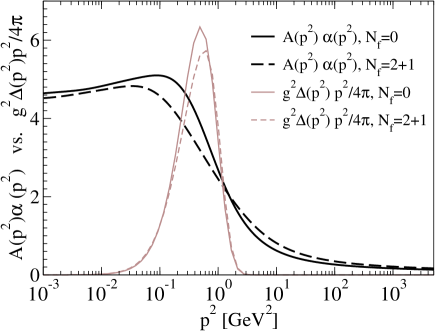
Figure 4: Comparison of the quenched and unquenched interactions used in the two models. In the full-SDE framework the interaction is given by the product $A(p^{2})\alpha(p^{2})$ whereas for the phenomenological model the equivalent function is $g^{2}\Delta(p^{2})p^{2}/4\pi$. The unquenching effects are calculated with physical sea-quarks, see tab. 2 for the corresponding values of the quark masses and interaction parameters.

The up/down and strange quark propagator functions for the full-SDE framework and for the phenomenological model are plotted in Fig. 5 and Fig. 6, respectively. Both sets of results for the quarks clearly exhibit a large degree of dynamical chiral symmetry breaking in the infrared region and we see the aforementioned effects of a reduction of the light quark mass function in the infrared once quark-loops are taken into account. For large momenta the numerical solutions of the full-SDE setup reproduce the logarithmic running known from resummed perturbation theory (see Fischer:2003rp for a detailed discussion of the ultraviolet properties of the quark mass function). Clearly, with the effective interaction of the phenomenological model being localised in the mid-momentum region, these asymptotic behaviours are not present. For intermediate momenta for all the quark flavors, we observe noticeable unquenching effects for the full-SDE setup which are not present in the phenomenological model. In the infrared, the effect of unquenching is that $Z_{f}(p^{2})$ is raised slightly and $M(p^{2})$ is lowered in all cases. There is, in addition, a striking difference in the behaviour of the quark wave function $Z_{f}(p^{2})$ when comparing the two models (though the unquenching effects are similar to both). In the up-quark of the phenomenological model, the localised interaction results in bending $Z_{f}$ back upwards as one moves into the infrared region. This effect is suppressed for the strange quark.

     

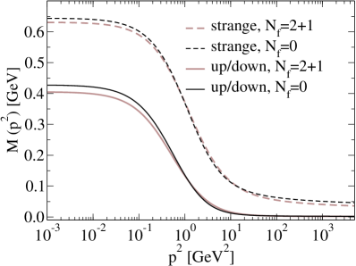
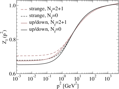
Figure 5: Comparison of the quenched and unquenched quark mass and wave-functions (left and right panels respectively) for the full-SDE setup. See text for details of the parameter configurations.

     

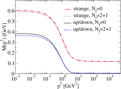
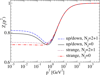
Figure 6: Comparison of the quenched and unquenched quark mass and wave-functions (left and right panels respectively) for the phenomenological model. See text for details of the parameter configurations.

The last point of note concerns possible singularities in the quark functions in the complex plane. These can readily be identified with our technique for calculating the quark functions in the complex plane (see appendix C), or using Schwinger-function techniques Alkofer:2003jj . We find that the nearest singularities to the origin occur as pairs of complex conjugate poles in the timelike region. For the chiral quarks of the phenomenological model they are found at roughly $(-0.26\pm 0.17\imath)\mathrm{GeV}^{2}$ (quenched) and $(-0.23\pm 0.13\imath)\mathrm{GeV}^{2}$ (unquenched), whereas for the finite mass quarks they are further out in the timelike region. With the full-SDE setup the poles are further away in the timelike region as compared with the phenomenological model and there is little difference between the quenched and unquenched cases. The likely explanation for the full-SDE poles being further from the origin is again the observation that the associated interaction is not localised to a specific region but rather extends throughout the full momentum range. We conclude that the unquenching has a slight effect on the position of the singularities but will not affect the BSE calculations of later sections. Indeed it has been checked during the numerical calculations that no singularities appear within the boundaries of the integration region associated with the BSE for any of the results shown in the paper.

IV.3 Numerical Results for Mesons: Physical quark masses, $N_{f}=2+1$

In this subsection we investigate two scenarios: quenched and unquenched with three physical quark masses, i.e. two light quarks representing the up/down quark and one heavier quark representing the strange quark. (Our results for three degenerate quark masses are presented in the next subsection.)

To start, let us explain how we determine physical observables. In the case of the full-SDE setup we have to use one experimental quantity (here the pion decay constant $f_{\pi}=130.7\,\mathrm{MeV}$) to convert the scale generated by dimensional transmutation to physical units. Furthermore we determine the quark masses $m_{u/d}$ and $m_{s}$ by the pseudoscalar observables $m_{\pi}=139.6\,\mathrm{MeV}$ and $m_{K}=493.7\,\mathrm{MeV}$ Eidelman:2004wy . To roughly compare with the values of the particle data group we determine $m_{u/d}$ and $m_{s}$ from the quark mass function at large momenta and subsequently evolve them down to $\mu=2\,\mathrm{GeV}$. To this end we extract the one-loop scale $\Lambda_{\widetilde{MOM}}^{N_{f}=0}=0.95\,\mbox{GeV}$ and $\Lambda_{\widetilde{MOM}}^{N_{f}=3}=1.09\,\mbox{GeV}$ from the ultraviolet behaviour of the running coupling. Note that we have employed a $\widetilde{MOM}$ scheme, thus these scales have the expected magnitude. In the case of the phenomenological model the scale is set by the paramater $d$ in the effective interaction, where in addition we take the fixed value $\omega=0.5\,\mathrm{GeV}$ and $\mu=1\,\mathrm{GeV}$. In order not to obscure the present discussion, details of the procedure for fitting $\mu$ are given in Appendix D. The quark masses are determined by fitting to the experimental pion and kaon masses.

The final values for the parameter sets with the resulting pseudoscalar meson masses, leptonic decay constants and vector meson masses are given in Table 2. When fitted to the experimental pion and kaon masses the resulting up/down and strange-quark masses are lowered when quark loop effects are taken into account. This has also been observed in corresponding lattice simulations CP-PACS ; JLQCD . We furthermore see that the results for $f_{K}$ and $m_{\rho}$ are quite insensitive to whether or not the system is unquenched. This leads to the conclusion that once the interaction has been fitted to the observable pseudoscalar observables, the vector meson mass is largely fixed. The likely explanation for this is that the ground state pseudoscalar and vector mesons are both states with the lowest orbital angular momentum ($L=0$) in the sense of the naive (quantum mechanical) quark model – meaning that they are determined largely by the lowest spin contributions of the BS kernel given by the ladder approximation. The interaction then plays the same role in both channels, hence the similarity in results. Note that the $\rho$ meson calculated within the framework of the truncated Bethe-Salpeter equation here refers to a pure quark-antiquark meson with no allowed decay channel - the physical $\rho$ meson has a non-trivial decay width. Thus, one must allow for some change in the calculated mass if one were to take the decay process into account. However, our results for $m_{\rho}$, especially in the full-SDE setup do seem low, although not unreasonable.

Table 2: Parameter sets and results for $m_{\pi}$, $f_{\pi}$, $m_{K}$ $f_{K}$ and $m_{\rho}$ for the quenched case ($N_{f}=0$), the unquenched case with three degenerate ’sea’-quarks ($N_{f}=3$) and the physical quark configuration case ($N_{f}=2+1$) with two up/down quarks and one strange quark. In the phenomenological model $\omega=0.5\,\mathrm{GeV}$ is held fixed and $\mu=1\,\mathrm{GeV}$. In the full-SDE setup we give values for the quark masses read off at a large scale and evolved down to $\mu=2\,\mathrm{GeV}$ according to their one-loop behaviour.

	$d$($\mathrm{GeV}^{-2}$)	$m_{u}$($\mathrm{MeV}$)	$m_{s}$($\mathrm{MeV}$)	$m_{\pi}$($\mathrm{MeV}$)	$f_{\pi}$($\mathrm{MeV}$)	$m_{K}$($\mathrm{MeV}$)	$f_{K}$($\mathrm{MeV}$)	$m_{\rho}$($\mathrm{MeV}$)
model:
$N_{f}=0$	14.92	5.26	117.5	139.6	130.7	493.7	152.4	737.6
$N_{f}=3$	16.94	5.17		139.6	130.7			734.7
$N_{f}=2+1$	16.66	5.18	116.4	139.6	130.7	493.7	153.0	735.0
	$\Lambda_{MOM}$($\mathrm{GeV}$)	$m_{u}^{2GeV}$($\mathrm{MeV})$	$m_{s}^{2GeV}$($\mathrm{MeV}$)	$m_{\pi}$($\mathrm{MeV}$)	$f_{\pi}$($\mathrm{MeV}$)	$m_{K}$($\mathrm{MeV}$)	$f_{K}$($\mathrm{MeV}$)	$m_{\rho}$($\mathrm{MeV}$)
full-SDE:
$N_{f}=0$	0.95	4.17	88.2	139.7	130.9	494.5	165.6	708.0
$N_{f}=3$	1.16	4.06		139.7	130.8			690.0
$N_{f}=2+1$	1.09	4.06	86.0	140.0	131.1	493.3	169.5	695.2
PDGEidelman:2004wy				139.6	130.7	493.7	160.0	770

IV.4 Numerical Results for Mesons: Degenerate quark masses, $N_{f}=3$

Let us now consider the degenerate quark configuration case, with $N_{f}=3$ identical quarks. To fit the parameters, we use a similar approach as that for the physical case, fitting to the pseudoscalar sector, though only the pion observables are relevant since there are no kaons. The parameters used and the resultant pion observables, along with the $\rho$ meson mass are shown in Table 2. We see that the unquenched results for $m_{\rho}$ are only slightly changed by the different unquenching configuration.

To further study the effects of unquenching we take the quenched and degenerate unquenched parameter configurations and plot the pseudoscalar and vector meson masses as a function of the quark mass parameter, keeping all other parameters fixed. The results are shown in Fig. 7. We see that for the full-SDE setup, both the pseudoscalar and vector masses with larger quark masses are increased $\sim 30\mathrm{MeV}$ when we include the unquenching effects. For the phenomenological model we see the same trend though the effect is less pronounced. Notice that as $m_{q}\rightarrow 0$ (the chiral limit) in both models, the pseudoscalar meson mass vanishes in accordance with the chiral symmetry considerations. This is a good check that the AXWTI has been faithfully maintained throughout the numerical procedure.

     
     

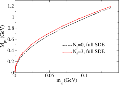
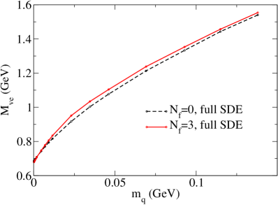
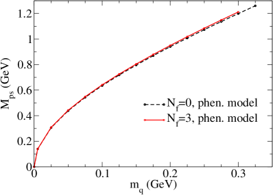
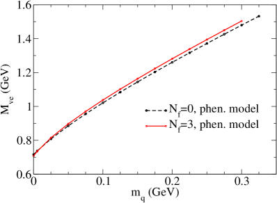
Figure 7: Pseudoscalar (left panels) and vector (right panels) meson masses as functions of the quark mass parameter. We compare the quenched and degenerate unquenched cases for both the full-SDE (upper panels) and phenomenological model (lower panels). Recall that there is no direct comparison between the quark masses of the full-SDE and phenomenological model.

Given the differences in the models, one is led to investigate in more detail the relationship between the meson masses, the interaction and the quark mass functions and how this relationship is altered when the quark loop is included. We plot the quark mass function at $p^{2}=0$ as a function of the quark mass parameter in Fig. 8. This serves to give a measure on the effect of unquenching for finite mass parameter quarks. We also plot in Fig. 9 the difference between the meson masses and twice the quark mass function $M(p^{2}=0)$. In the static, quantum mechanical model of mesons this would be interpreted as a binding energy due to the interaction. We point out, however, that in the (relativistic) Bethe-Salpeter approach here this interpretation does not hold. We shall refer to this difference as the ’binding’ but the reader should bear in mind that this is a loose definition of the term. We see that in Fig. 9 the unquenching does indeed have a significant effect on the internal behaviour of the BSE.

     

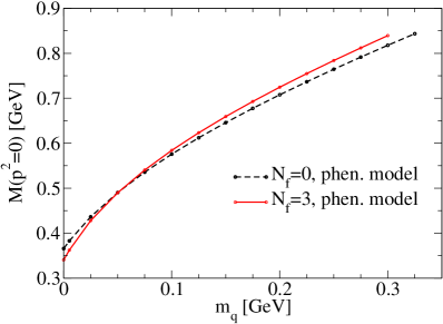
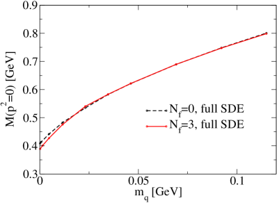
Figure 8: Quark mass function at $p^{2}=0$ as a function of the quark mass parameter. We compare the quenched and degenerate unquenched cases.

     
     

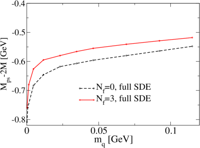
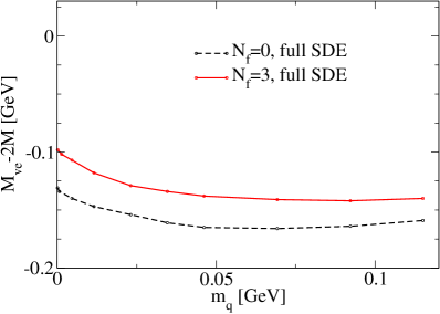
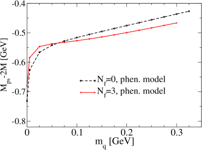
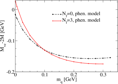
Figure 9: The difference between the pseudoscalar (left panel) and vector (right panel) meson masses and twice the quark mass function $M(p^{2}=0)$ as functions of the quark mass parameter. We compare the quenched and degenerate unquenched cases.

Expressed in the form of figs. 8 and 9 one can now clearly see the difference in the two models. In the full-SDE setup at finite quark masses the quark mass function becomes insensitive to unquenching. This can be intuitively explained because the quark loops become suppressed by their mass. However, the overall meson masses show a $\sim 30\mathrm{MeV}$ increase, reflected in the binding. Thus in the full-SDE setup, the unquenching of the interaction has an effect in the BSE but not in the quark mass function.

In distinction, for the phenomenological model the situation is more complex. At low quark masses the quark mass functions and the binding do show the same behaviour as for the full-SDE setup - but of course for low quark masses all mesons are in the vicinity of the fixed physical point from which the parameters are fitted. As one increases the quark mass though, the curves for the quenched and unquenched quark mass functions and binding cross. Looking at the parameter sets, one sees that in the unquenched case the overall magnitude $d$ is larger. As the quark masses are increased, the quark loop becomes suppressed and one is left with a stronger interaction, hence the increased quark mass function. (Recall that in the full-SDE setup there is no fitted parameter corresponding to the overall magnitude, hence the different behaviour of the quark mass function). Since for small $m_{q}$ the unquenched mass function is lower than the quenched case eventually the curves cross. However, the meson mass does not increase so significantly under unquenching for larger $m_{q}$, even though both the interaction and the quark mass function do increase. The resolution to this apparent dichotomy lies in the fact that for larger quark mass parameters, the relative contribution of the bare quark mass to the total meson mass is greater and the effect of increasing the interaction and quark mass function is damped (recall that the quark mass function referred to here is $M(p^{2}=0)$).

This discussion of the detailed effects of unquenching serves to highlight that we are not dealing with a system where the total mass is given by the sum of the constituent masses and their binding energy but rather with a relativistic system whose constituents all depend non-trivially upon each other and crucially, all the components have varying effects at different momentum scales. The two models exhibit different behaviour when quark loops are included and this is because of the different forms of the interaction. The overall properties of the meson masses are largely determined by the integrated strength of the interaction. However, the closer inspection of unquenching for finite quark masses does indeed reveal that the form of the interaction plays a role.

Finally, we make contact again to corresponding lattice calculations CP-PACS ; JLQCD . Since it is most conclusive to compare ’physical’ quantities we plot the vector meson masses vs. the corresponding pseudoscalar meson masses. For large quark masses one may expect that unquenching effects in these quantities will be mainly determined by the interaction alone, since the decay of the vector meson to two pseudoscalar mesons is no longer kinematically allowed (though in principle unquenching effects involving vertex corrections beyond the truncation schemes discussed here may also play a role). The comparison to the lattice is therefore a genuine test of our two setups. From the plot in Fig. 10 we find good agreement between the curves from both of our setups and the available lattice data. It is apparent that the effects due to unquenching are smaller than both the differences due to the different truncation schemes and the systematic errors of the lattice results. Because we are plotting the more physical meson masses and not the (incomparable) quark mass parameters, the difference between the quenched and unquenched curves for both of our setups becomes the same – the curve for the unquenched vector meson mass as a function of the pseudoscalar meson mass is slightly raised for large values of the pseudoscalar meson mass. For small masses we observe a nonlinear relation of the two masses reflecting the different roles of the vector and the pseudoscalar meson sector in chiral limit.

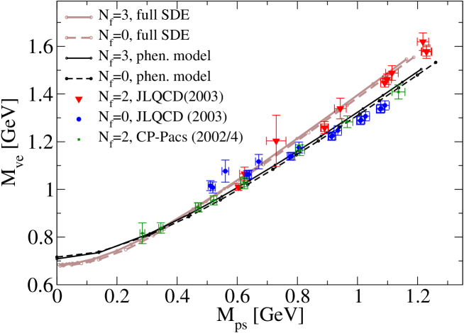
Figure 10: Vector meson masses as a function of pseudoscalar meson masses. We compare the quenched and degenerate unquenched cases. The lattice results are taken from refs. CP-PACS ; JLQCD .

V Summary and Conclusions

We have investigated the effects of unquenching the gluon polarisation when applied to the Bethe–Salpeter framework for light pseudoscalar and vector meson masses. To obtain model-independent information on these effects we considered two distinct methods of calculating the corresponding gluon and quark propagators self-consistently. The first uses a sophisticated truncation of the Schwinger–Dyson equations for the ghost, gluon and quark propagator. The second uses a (simpler) phenomenologically motivated form for the quenched Yang-Mills sector of the theory. In both approaches, we explicitly took quark loop contributions to the gluon polarisation into account. Employing the resultant propagator functions in conjunction with a truncation for the Bethe–Salpeter equation we calculated light pseudoscalar and vector meson masses. The forms of the truncated Bethe–Salpeter kernel are such that the axialvector Ward-Takahashi identity for color singlet, flavor non-singlet channels is obeyed, thereby ensuring that the generic features of the chiral limit of the pseudoscalar meson sector are manifest. Though the resulting effective quark-gluon interactions in our two approaches are rather different, both produce similar qualitative effects in meson observables. This finding enforces our general belief that the lowest meson states are dominated by the pattern of dynamical chiral symmetry breaking and are not largely affected by the detailed structure of the interaction.

We observed sizeable unquenching effects due to the inclusion of quark loops to the gluon polarisation at various stages of our investigation. For the ghost and gluon propagator functions, calculated in the full Schwinger–Dyson truncation scheme, these effects occur predominantly in the intermediate momentum region. At momenta around $1\mathrm{GeV}$ the screening of quark-antiquark pairs moderates the bump in the gluon propagator considerably, whereas the infrared behaviour of both propagators is unaffected. For the quark propagator functions we found slight effects also in the infrared: the quark mass and wave functions for up/down and strange quark masses are reduced by about 10% when unquenched. These results agree with previous findings Fischer:2003rp and have recently been confirmed in lattice simulations Bowman:2004jm ; Bowman:2005vx . We determined the location of the singularities of the quark propagator in the complex momentum plane and found a pair of complex conjugated poles, which are hardly affected by the inclusion of quark loop effects. Furthermore we found only very small changes in the chiral condensate as long as the number of flavors $N_{f}\leq 3$, indicating a large critical number of flavors for the chiral phase transition. All these effects are model independent in the sense that we observed them in the full SDE-setup as well as in our phenomenological model (where assessible).

The main focus of the present work has been on the spectrum and decay constants of pseudoscalar and vector mesons. Here, the physical pion and kaon masses along with the pion leptonic decay constant have been used to determine the scale of the interaction as well as the up/down and strange quark masses. The resulting masses at the physical point are smaller when quark loop effects are taken into account. Again this agrees with observations in corresponding lattice simulations CP-PACS ; JLQCD . The kaon leptonic decay constant and vector meson mass were in rough agreement with available data, whereas the vector meson mass turned out slightly too low. The vector mass is subject to corrections due to a finite rho decay width Watson:2004jq and further structure in the quark-gluon vertex Bhagwat:2004hn ; Watson:2004kd , which both were beyond the scope of the present work. Importantly however, our results for $f_{K}$ and $m_{\rho}$ were not significantly altered when quark loops were included.

To further discuss the role of the quark loop contribution to the gluon polarisation, we compared quenched and unquenched mesons with degenerate sea-quark configurations. Keeping the scale of the interaction fixed, we studied the quark mass function as well as the pseudoscalar and vector meson masses as functions of the quark mass parameter. As expected, both of our approaches preserve the Goldstone character of the pion in the chiral limit. For small quark masses the observables depend nonlinearly on the quark mass parameter. For large quark masses the two schemes display different behaviour under unquenching. The full Schwinger–Dyson truncation results exhibit an increase in the meson masses when quark loops are included, whereas for the phenomenological model this increase is much smaller.

Furthermore we studied the vector meson masses as a function of the pseudoscalar meson mass and compared with recent lattice results from various groups. The resultant curves for the two schemes, though different from each other, are nonetheless in general agreement with the lattice data. For pion masses below 240 MeV, where no lattice data are available, our results show a nonlinear dependence of the vector meson mass on the pseudoscalar one. The effect of unquenching – when viewed as a function of the pseudoscalar meson mass – becomes the same for both schemes: the vector meson mass is slightly increased when quark loops are taken into account. This trend is also seen in the lattice simulations CP-PACS ; JLQCD , where the effect is even more pronounced. However, these unquenching effects are small compared to the differences between both the truncation schemes we employed and the systematic errors of the lattice results.

Appendix A Conventions for Renormalisation in the full SDE Truncation Scheme

In the full Schwinger–Dyson equation truncation, renormalised dressing functions are denoted by an overbar. They are related to their unrenormalised counterpart via the renormalisation constant $Z_{i}(\mu,\Lambda)$ where $\mu$ is the renormalisation scale and $\Lambda$ is the regularisation scale. The multiplicative renormalisation constants are defined as follows:

$$S(p,\Lambda) = Z_{2}(\mu,\Lambda)\overline{S}(p,\mu)~{}~{}~{},$$ (55)

$$D(p,\Lambda) = Z_{3}(\mu,\Lambda)\overline{D}(p,\mu)~{}~{}~{},$$ (56)

$$G(p,\Lambda) = \tilde{Z}_{3}(\mu,\Lambda)\overline{G}(p,\mu)~{}~{}~{},$$ (57)

$$\Gamma_{\rho}(p_{i},\Lambda) = Z_{1F}^{-1}(\mu,\Lambda)\overline{\Gamma}_{\rho}(p_{i},\mu)~{}~{}~{},$$ (58)

$$\tilde{\Gamma}_{\rho}(p_{i},\Lambda) = \tilde{Z}_{1}^{-1}(\mu,\Lambda)\overline{\tilde{\Gamma}}_{\rho}(p_{i},\mu)~{}~{}~{},$$ (59)

$$\Gamma_{\rho\nu\lambda}(p_{i},\Lambda) = Z_{1}^{-1}(\mu,\Lambda)\overline{\Gamma}_{\rho\nu\lambda}(p_{i},\mu)~{}~{}~{}.$$ (60)

The renormalised fermion mass function is obtained with the relation $Z_{2}M_{\Lambda}=Z_{4}\overline{M}_{p}$ and the running quark mass $\overline{M}_{p}$ is independent of the renormalisation scale $\mu$. The coupling is renormalised according to

$$g^{2}(\Lambda)=\frac{\tilde{Z}_{1}^{2}}{Z_{3}\tilde{Z}_{3}^{2}}\overline{g}^{2}(\mu)$$ (61)

and the Slavnov-Taylor identity, which ensures the universality of the renormalised coupling, is expressed as

$$\frac{Z_{3}}{Z_{1}}=\frac{\tilde{Z}_{3}}{\tilde{Z}_{1}}=\frac{Z_{2}}{Z_{1F}}~{}~{}~{}.$$ (62)

Appendix B A Truncation of the ghost and gluon SDEs

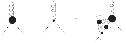
Figure 11: Ghost-gluon vertex DS equation.

Here we shortly summarise the truncation for the ghost- and gluon-SDEs as introduced in refs. Fischer:2002hn ; Fischer:2003rp ; Fischer:2003zc . In order to close the Eqs. (11) and (12) we have to specify expressions for the ghost-gluon vertex, the three-gluon vertex and the four-gluon vertex. Our ansatz for the quark-gluon vertex has been discussed in the main body of this work, cf. Eq.(10).

The crucial property of the ghost-gluon vertex

$$\Gamma_{\mu}^{abc}(p,q)=\Gamma_{\mu}(p,q)f^{abc}$$ (63)

is that both, incoming and outgoing ghost momentum factorise in Landau gauge Taylor:ff . Indeed, factorisation of the outgoing ghost momentum $p$ is immediate and occurs in all linear covariant gauges. Factorisation of the incoming ghost momentum $q$ can be seen easily from its Schwinger–Dyson equation, Fig. 11, and the transversality of the gluon propagator $D_{\mu\nu}$, which implies that $l_{\mu}D_{\mu\nu}(l-q)=q_{\mu}D_{\mu\nu}(l-q)$. Thus, provided the gluon-ghost kernel in Fig. 11 is well behaved in the infrared (i.e. not too singular), we obtain a bare vertex for $q_{\mu}\rightarrow 0$. Indeed at least one self-consistent infrared solution of the whole tower of SDE exists Alkofer:2004it , in which the gluon-ghost kernel indeed is singular, but not singular enough to spoil the argument. If this is true, then a bare ghost-gluon vertex

$$\Gamma_{\mu}(q,p)=iq_{\mu}$$ (64)

provides a good approximation to the full vertex in the infrared and also in the ultraviolet region of momentum. Indeed, recent lattice calculations Cucchieri:2004sq and also a study in the SDE-approach Schleifenbaum:2004id support this approximation.

One knows from the self-consistent infrared solution Alkofer:2004it , that the ghost-loop is the leading diagram of the gluon-SDE in the infrared. Although the three-gluon and four-gluon vertices are singular in this scenario, they are not singular enough to overcome the suppression induced by the gluon dressing functions. Thus effects from the four-gluon vertex on the gluon-propagator are negligible in the infrared. As they are also subleading in the ultraviolet and moreover are technically complicated to evaluate we neglect these effects from the start by choosing the four-gluon vertex to be zero.

On the other hand, although the effects from the gluon-loop including the three-gluon vertex are also negligible in the infrared, they contribute to the one-loop running of the propagator in the ultraviolet and have considerable impact on the mid-momentum behaviour of the propagator. One therefore has to include a suitable ansatz for the three-gluon vertex. Such an ansatz has been constructed and investigated in refs. Fischer:2002hn ; Fischer:2003rp ; Fischer:2003zc and is given by

$$\Gamma_{\mu\nu\lambda}^{abc}(k,p,q)=\Gamma_{\mu\nu\lambda}^{abc,0}(k,p,q)H_{3g}(k,p,q)$$ (65)

where $\Gamma_{\mu\nu\lambda}^{abc,0}(k,p,q)$ is the bare vertex. The dressing function $H_{3g}$ is given by

$$H_{3g}(k,p,q)=\frac{1}{Z_{1}}\frac{G(q)^{(-2-6\delta)}}{Z(q)^{(1+3\delta)}}\frac{G(p)^{(-2-6\delta)}}{Z(p)^{(1+3\delta)}}\;,$$ (66)

with the momenta $q$ and $p$ running in the loop. Here the anomalous dimension of the ghost propagator, $\delta=-9N_{c}/(44N_{c}-8N_{f})$, together with the vertex renormalization constant $Z_{1}$ ensure the correct ultraviolet running of the vertex with momenta and renormalization scale. Furthermore this choice leads to cutoff independent ghost and gluon dressing functions in the continuum.

Appendix C Solving the SDE in the Complex Plane

In the (Euclidean space version of the) Bethe-Salpeter equation, one is looking for a solution $P^{2}=-M^{2}$ which necessarily introduces complex momenta into the problem. The quark propagator must be evaluated at momenta within a parabola $k^{2}-M^{2}/4\pm\imath\sqrt{k^{2}M^{2}}$ in the complex plane. In order to achieve this, we must solve the coupled quark and gluon propagator SDEs in the complex plane and we shall do this using a combination of contour integrals and UV asymptotic expansion. Expanding the integral measure and paying attention to the flavor index $i$, the coupled equations (24,23,22) become

$$a^{i}(x) = 1+\frac{4}{3(2\pi)^{3}}\int_{0}^{\infty}dy\,y\int_{-1}^{1}dz\sqrt{1-z^{2}}\,g^{2}\Delta(y)v^{i}(x+y-2\sqrt{xy}z)\left[1-3{\frac{\sqrt{y}}{\sqrt{x}}}z+2z^{2}\right],$$ (67)

$$b^{i}(x) = m^{i}+\frac{4}{3(2\pi)^{3}}\int_{0}^{\infty}dy\,y\int_{-1}^{1}dz\sqrt{1-z^{2}}\,g^{2}\Delta(y)s^{i}(x+y-2\sqrt{xy}z)\left[3\right],$$ (68)

$$\Sigma(x) = \sum_{i=u,d,s}\frac{4}{3(2\pi)^{3}}\int_{0}^{\infty}dy\,y\int_{-1}^{1}dz\sqrt{1-z^{2}}v^{i}(y)v^{i}(x+y-2\sqrt{xy}z)\left[\frac{y}{x}(1-4z^{2})+3\frac{\sqrt{y}}{\sqrt{x}}z\right],$$ (69)

where $x=p^{2}$, $y=k^{2}$ and $z=p\!\cdot\!k/\sqrt{p^{2}k^{2}}$. Alternatively, one can choose a symmetric momentum routing. Equations (67,68,69) then become

$$a^{i}(x) = 1+\frac{4}{3(2\pi)^{3}}\int_{0}^{\infty}dy\,y\int_{-1}^{1}dz\sqrt{1-z^{2}}\,g^{2}\Delta(y_{-})v^{i}(y_{+})\left[-\frac{1}{2}+3{\frac{\sqrt{y}}{\sqrt{x}}}z+2\frac{x/4+yz^{2}-\sqrt{xy}z}{x/4+y-\sqrt{xy}z}\right],$$ (70)

$$b^{i}(x) = m^{i}+\frac{4}{3(2\pi)^{3}}\int_{0}^{\infty}dy\,y\int_{-1}^{1}dz\sqrt{1-z^{2}}\,g^{2}\Delta(y_{-})s^{i}(y_{+})\left[3\right],$$ (71)

$$\Sigma(x) = \sum_{i=u,d,s}\frac{4}{3(2\pi)^{3}}\int_{0}^{\infty}dy\,y\int_{-1}^{1}dz\sqrt{1-z^{2}}v^{i}(y_{-})v^{i}(y_{+})\left[\frac{y}{x}(1-4z^{2})+\frac{3}{4}\right],$$ (72)

where $y_{\pm}=x/4+y\pm\sqrt{xy}z$. The reason for the two momentum routings is the following: At large values of the radial integral variable $y$, the asymmetric momentum routing has factors of either $g^{2}\Delta(y)$ or $v^{i}(y)$ which vanish quickly for large $y$. The fidelity of the angular integration is thus less important even when $x$ and $y$ are both large (large $x$ here refers to spacelike momenta). In the symmetric case at large $x$ and $y$, the angular integration involves integrating over functions which vary considerably over the entire momentum range and so is numerically much more difficult. For this reason, although the two sets of equations are formally equivalent (ignoring for now the possible complications of the UV-cutoff), numerically we use the asymmetric routing at large $x$ such that the angular integral can be more readily done. The use of the symmetric routing comes about in the context of the contour integrals below.

Let us now describe how the equations are solved in the complex plane. At large $\Re{x}$ the functions take asymptotic forms

$$a(x) \stackrel{{\scriptstyle x\rightarrow\infty}}{{=}} 1+\sum_{k=1}^{N}\frac{a_{k}}{x^{k}},$$ (73)

$$b(x) \stackrel{{\scriptstyle x\rightarrow\infty}}{{=}} m+\sum_{k=1}^{N}\frac{b_{k}}{x^{k}},$$ (74)

$$\Sigma(x) \stackrel{{\scriptstyle x\rightarrow\infty}}{{=}} \sigma_{0}\log{x}+\sum_{k=1}^{N}\frac{\sigma_{k}}{x^{k-1}}.$$ (75)

For a given set of coefficients one can extrapolate these functions at arbitrary $x$ to the complex region, as long as $\Re{x}$ is large. Now consider the contour defined by the lines (shown in Fig. 12)

$$z_{-}(t)= -x_{0}+t-2\imath\sqrt{x_{0}t}, t=[\varepsilon,\lambda],$$

$$z_{\lambda}(r)= -x_{0}+\lambda+2\imath\sqrt{x_{0}\lambda}r, r=[-1,1],$$

$$z_{+}(t)= -x_{0}+t+2\imath\sqrt{x_{0}t}, t=[\lambda,\varepsilon],$$

$$z_{\varepsilon}(r)= -x_{0}+\varepsilon-2\imath\sqrt{x_{0}\varepsilon}r, r=[-1,1].$$ (76)

Figure 12: Sketch of the closed contour in the complex $z$ plane.

With these definitions the integral measure along the closed contour is:

$$\oint_{c}dz\rightarrow\int_{\varepsilon}^{\lambda}dt(1-\imath\sqrt{x_{0}/t})+2\imath\sqrt{x_{0}\lambda}\int_{-1}^{1}dr-\int_{\varepsilon}^{\lambda}dt(1+\imath\sqrt{x_{0}/t})-2\imath\sqrt{x_{0}\varepsilon}\int_{-1}^{1}dr.$$ (77)

For $z_{1}$ within the contour the Cauchy integral formula holds:

$$2\pi\imath f(z_{1})=\oint_{c}dz\frac{f(z)}{z-z_{1}},$$ (78)

so given the function on the contour one can derive its value at some arbitrary interior point. Notice that numerically this is easy to implement as long as $z_{1}$ is not close to the contour itself.

Turning to the above coupled system of SDEs we supply a set of starting functions $a^{i}$, $b^{i}$ and $\Sigma$ along the contour and along the spacelike axis, from which one can obtain the asymptotic expansion coefficients. From this we can derive the functions $v^{i}$, $s^{i}$ and $g^{2}\Delta$ using the expansion (for large real parts of the argument) or the contour integration (for small arguments) at those values needed to form the integrands of the coupled equations. With this we can then recalculate the functions on the left-hand side of the equations for external $x$ again around the contour or on the spacelike axis. This gives us an iterative procedure to solve the system of equations. As explained above, we use the asymmetric momentum routing for large $\Re{x}$. However, for small $\Re{x}$ we use the symmetric routing since for some point $x$ on the contour we now need the integrand functions at points within the smaller parabola associated with $x/4$ and hence well inside the contour. This ensures that the Cauchy integral formula can be reliably implemented. It also means that if $v^{i}$ and $s^{i}$ are singular in the complex region, we can spot this by choosing the contour such that the singularity lies between the contour of external $x$ and the smaller parabolic domain accessed by the integrands.

We point out that within the iterative procedure there is no interpolation needed, except for the asymptotic region where the functions are well known and slowly varying. Certainly an interpolating scheme could not, even in principle, be used in regions where there are singularities present. In addition, the contour integrals are quick, simple to set up and are more accurate than an interpolation. The last point is the usefulness of the method in solving the BSE – given the converged solution to the SDEs along the spacelike axis and around the contour, one can then obtain the quark functions at any point needed within the parabolic BSE domain directly.

The various parameters associated with the numerical implementation are as follows. The tip of the contour is given by the parameter $\varepsilon=0.1\mathrm{GeV}^{2}$ (avoiding the integrable square-root singularity to make the numerics easier), whereas the end is given by $\lambda=11\mathrm{GeV}^{2}$. $\Re{x}\geq 10\mathrm{GeV}^{2}$ is ’large’ and we use the asymptotic expansion. There a numerical limit to how large the overall contour parameter, $x_{0}$, which defines the size of the complex region that the system accesses can be and this comes from the requirement that the contour integral be reliable and reasonably fast. In practice it is found that $x_{0}\leq 0.3\mathrm{GeV}^{2}$ works well. If quark propagators are needed outside this domain then one can use the SDE with symmetric routing to evaluate the functions, given the solution within. This gives an upper limit to the domain of applicability of the technique but this is due to the numerical implementation, not the technique itself.

Appendix D Discussion of the renormalisation point dependence of the phenomenological model

In the phenomenological model, the renormalisation scale $\mu$ is a free parameter to be fitted. Since the model is not fully multiplicatively renormalisable, the results do in general depend on $\mu$. We show here how $\mu$ is constrained. Let us begin by considering the behaviour of the chiral condensate defined by Eq. (54) and additionally an approximation to the pion leptonic decay constant in the chiral limit Watson:2004kd

$$\left(f_{\pi}^{0}\right)^{2}=\frac{3}{2\pi^{2}}\int_{0}^{\infty}dy\frac{yb_{y}}{(ya_{y}^{2}+b_{y}^{2})^{2}}\left[a_{y}b_{y}-\frac{y}{2}(a_{y}b_{y}^{\prime}-b_{y}a_{y}^{\prime})\right].$$ (79)

It is known that this approximation underestimates $f_{\pi}$ by around $10\%$. We calculate $f_{\pi}^{0}$ for a range of $\mu$ whilst using $<\overline{q}q>^{0}$ to fit $d$ with $\omega=0.5\mathrm{GeV}$ fixed in order to constrain the range of $\mu$. The results are shown in Table 3. We see that there is a mild decrease in $f_{\pi}^{0}$ as $\mu$ increases. For large values of $\mu$ we see that $d$ must be increased dramatically in order to generate the same degree of dynamical symmetry breaking given by $<\overline{q}q>^{0}$. Conversely, for small values of $\mu$ ($<0.7\mathrm{GeV}^{2}$), $d$ must be smaller than the quenched value. This is not unnatural if one considers that in the model the typical scale is $\sim 1\mathrm{GeV}$ – renormalisation at a scale greater larger or smaller is not physical. From the lattice results displayed in Fig. 3 and the results of the full-SDE truncation shown also in Fig. 4, it is expected that the unquenching of the system reduces the gluon dressing by $\sim 10\%$ and this indicates that $\mu\sim 1.0\mathrm{GeV}^{2}$ is a physical choice.

Table 3: Parameter sets and calculated $<\overline{q}q>^{0}$ and $f_{\pi}^{0}$ (chiral limit) using the phenomenological model. $\omega=0.5\mathrm{GeV}$ is held fixed.

	$d$ ($\mathrm{GeV}^{-2}$)	$\mu$ ($\mathrm{GeV}^{2}$)	$-(<\overline{q}q>^{0})^{1/3}$ ($\mathrm{MeV}$)	$f_{\pi}^{0}$ ($\mathrm{MeV}$)
quenched	16.0	—	251.2	118.9
	13.0	0.2	251.4	119.2
	15.0	0.5	251.8	118.9
unquenched	16.2	0.7	251.4	118.3
($N_{f}=3$)	18.0	1.0	251.2	117.7
	24.0	2.0	251.0	116.2
	45.5	5.0	250.9	113.1

We present parameter sets and meson mass results for the physical ($N_{f}=2+1$) and degenerate ($N_{f}=3$) unquenching scenarios with varying values of $\mu$ in Table 4. From the insensitivity of the rho meson mass and the kaon leptonic decay constant, it is clear that fitting $\mu$ to either of these results is not a good procedure and the preceeding discussion of the interaction strength is more relevant to constrain $\mu$. The near-invariance of the meson masses with respect to $\mu$ is the remnant of the renormalisation scale invariance that observables should adhere to and that we observe it here is a good sign that the phenomenological treatment retains the character of the full theory, insofar as these observables are concerned.

Table 4: Parameter sets and resultant $m_{\pi}$, $f_{\pi}$, $m_{K}$ $f_{K}$ and $m_{\rho}$ for the phenomenological model. $\omega=0.5\mathrm{GeV}$ is held fixed.

	$\mu$($\mathrm{GeV}^{2}$)	$d$($\mathrm{GeV}^{-2}$)	$m_{u}$($\mathrm{MeV}$)	$m_{s}$($\mathrm{MeV}$)	$m_{\pi}$($\mathrm{MeV}$)	$f_{\pi}$($\mathrm{MeV}$)	$m_{K}$($\mathrm{MeV}$)	$f_{K}$($\mathrm{MeV}$)	$m_{\rho}$($\mathrm{MeV}$)
quenched	—	14.92	5.265	117.55	139.6	130.7	493.7	152.4	737.6
unquenched	1.0	16.66	5.185	116.4	139.6	130.7	493.7	153.0	735.0
($N_{f}=2+1$)	0.7	15.12	5.22	117.0	139.6	130.7	493.7	152.8	736.2
	1.3	18.67	5.14	5.14	139.6	130.7	—	—	733.2
unquenched	1.0	16.94	5.17	5.17	139.6	130.7	—	—	734.7
($N_{f}=3$)	0.7	15.15	5.22	5.22	139.6	130.7	—	—	735.8

Finally (and for the sake of completeness), using the quenched and degenerate ($N_{f}=3$) unquenched quark configuration scenarios (using the parameters of Table 4) we plot the vector meson mass as a function of the pseudoscalar meson mass in Fig. 13 for increasing quark mass parameter with different values of $\mu$ (cf. Fig. 10). Between all the cases it is seen that the unquenching is a small, though non-negligible effect. For $\mu=0.7\mathrm{GeV}^{2}$, where the parameter $d$ (from Table 4) is almost unchanged from the quenched case the unquenched results are almost identical to their quenched counterpart. For larger values of $\mu$ the effect due to unquenching becomes larger.

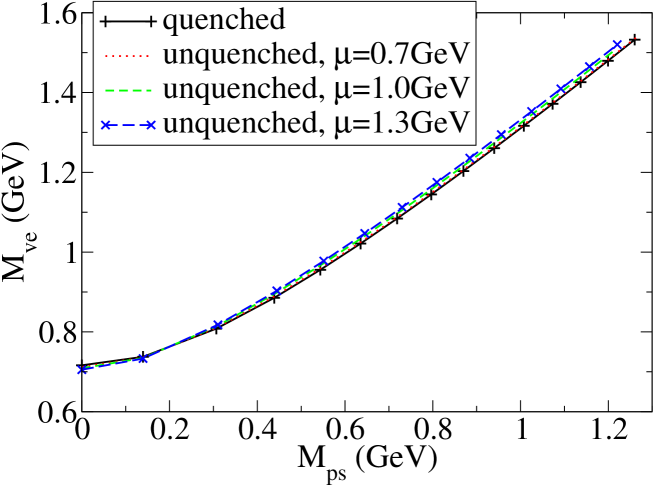
Figure 13: Vector meson masses as a function of pseudoscalar meson masses in the phenomenological model for different values of the renormalisation scale $\mu$. We compare the quenched and degenerate unquenched cases.

References

- (1) C. Itzykson, and J.-B. Zuber, ”Quantum Field Theory”, McGraw-Hill (1985).
- (2) R. Alkofer and L. von Smekal, Phys. Rept. 353 (2001) 281 [arXiv:hep-ph/0007355].
- (3) C. D. Roberts and S. M. Schmidt, Prog. Part. Nucl. Phys. 45 (2000) S1 [arXiv:nucl-th/0005064].
- (4) P. Maris and C. D. Roberts, Int. J. Mod. Phys. E 12, 297 (2003).
- (5) P. Maris, C. D. Roberts and P. C. Tandy, Phys. Lett. B 420, 267 (1998) [arXiv:nucl-th/9707003].
- (6) P. Maris and P. C. Tandy, Phys. Rev. C 60 (1999) 055214 [arXiv:nucl-th/9905056].
- (7) R. Alkofer, P. Watson and H. Weigel, Phys. Rev. D 65 (2002) 094026 [arXiv:hep-ph/0202053].
- (8) P. Maris and P. C. Tandy, Phys. Rev. C62, 055204 (2000) [arXiv:nucl-th/0005015].
- (9) J. Volmer, et al. (The Jefferson Lab F(pi) Collaboration), Phys. Rev. Lett. 86, 1713 (2001), [arXiv:nucl-ex/0010009].
- (10) P. Maris, PiN Newslett. 16, 213 (2002), [arXiv:nucl-th/0112022].
- (11) D. Jarecke, P. Maris, and P. C. Tandy, Phys. Rev. C67, 035202 (2003), [arXiv:nucl-th/0208019].
- (12) P. Maris and P. C. Tandy, Phys. Rev. C65, (2002) 045211, [arXiv:nucl-th/0201017].
- (13) C.-R. Ji, and P. Maris, Phys. Rev. D64, 014032 (2001), [arXiv:nucl-th/0102057].
- (14) A. Bender, W. Detmold, C. D. Roberts and A. W. Thomas, Phys. Rev. C 65 (2002) 065203 [arXiv:nucl-th/0202082].
- (15) M. S. Bhagwat, A. Holl, A. Krassnigg, C. D. Roberts and P. C. Tandy, Phys. Rev. C 70 (2004) 035205 [arXiv:nucl-th/0403012].
- (16) P. Watson, W. Cassing and P. C. Tandy, Few Body Syst. 35 (2004) 129 [arXiv:hep-ph/0406340].
-
(17)
C. S. Fischer and R. Alkofer,
Phys. Lett. B 536, 177 (2002)
[arXiv:hep-ph/0202202];
C. S. Fischer, R. Alkofer and H. Reinhardt, Phys. Rev. D 65 (2002) 094008 [arXiv:hep-ph/0202195]. - (18) C. S. Fischer and R. Alkofer, Phys. Rev. D 67 (2003) 094020 [arXiv:hep-ph/0301094].
- (19) P. Watson and W. Cassing, Few Body Syst. 35 (2004) 99 [arXiv:hep-ph/0405287].
-
(20)
L. von Smekal, R. Alkofer and A. Hauck,
Phys. Rev. Lett. 79 (1997) 3591
[arXiv:hep-ph/9705242];
L. von Smekal, A. Hauck and R. Alkofer, Annals Phys. 267 (1998) 1 [Erratum-ibid. 269, 182 (1998)] [arXiv:hep-ph/9707327]. -
(21)
D. Atkinson and J. C. R. Bloch,
Phys. Rev. D 58, 094036 (1998)
[arXiv:hep-ph/9712459];
D. Atkinson and J. C. R. Bloch, Mod. Phys. Lett. A 13 (1998) 1055 [arXiv:hep-ph/9802239]. - (22) P. Watson and R. Alkofer, Phys. Rev. Lett. 86 (2001) 5239 [arXiv:hep-ph/0102332].
- (23) D. Zwanziger, Phys. Rev. D 65, 094039 (2002).
- (24) C. Lerche and L. von Smekal, Phys. Rev. D 65, 125006 (2002) [arXiv:hep-ph/0202194].
- (25) D. Zwanziger, Phys. Rev. D 69 (2004) 016002 [arXiv:hep-ph/0303028].
- (26) R. Alkofer, C. S. Fischer and F. J. Llanes-Estrada, Phys. Lett. B 611, 279 (2005) [arXiv:hep-th/0412330].
- (27) P. Maris and C. D. Roberts, Phys. Rev. C 56, 3369 (1997) [arXiv:nucl-th/9708029].
- (28) J. C. R. Bloch, Phys. Rev. D 66, 034032 (2002) [arXiv:hep-ph/0202073].
- (29) M. S. Bhagwat, M. A. Pichowsky, C. D. Roberts and P. C. Tandy, Phys. Rev. C 68, 015203 (2003) [arXiv:nucl-th/0304003].
- (30) J. C. Taylor, Nucl. Phys. B 33 (1971) 436.
- (31) J. M. Pawlowski, D. F. Litim, S. Nedelko and L. von Smekal, Phys. Rev. Lett. 93, 152002 (2004) [arXiv:hep-th/0312324]; C. S. Fischer and H. Gies, JHEP 0410 (2004) 048 [arXiv:hep-ph/0408089].
- (32) D. B. Leinweber, J. I. Skullerud, A. G. Williams and C. Parrinello [UKQCD collaboration], Phys. Rev. D 58 (1998) 031501 [arXiv:hep-lat/9803015].
- (33) P. O. Bowman, U. M. Heller, D. B. Leinweber, M. B. Parappilly and A. G. Williams, Phys. Rev. D 70, 034509 (2004) [arXiv:hep-lat/0402032].
- (34) J. Gattnar, K. Langfeld and H. Reinhardt, Phys. Rev. Lett. 93, 061601 (2004) [arXiv:hep-lat/0403011].
- (35) O. Oliveira and P. J. Silva, AIP Conf. Proc. 756, 290 (2005) [arXiv:hep-lat/0410048].
- (36) A. Sternbeck, E. M. Ilgenfritz, M. Mueller-Preussker and A. Schiller, Phys. Rev. D 72 (2005) 014507 [arXiv:hep-lat/0506007].
- (37) C. S. Fischer, B. Gruter and R. Alkofer, arXiv:hep-ph/0506053.
- (38) C. S. Fischer and D. Zwanziger, Phys. Rev. D 72 (2005) 054005 [arXiv:hep-ph/0504244].
- (39) A. Bender, C. D. Roberts and L. Von Smekal, Phys. Lett. B 380 (1996) 7 [arXiv:nucl-th/9602012].
- (40) M. S. Bhagwat and P. C. Tandy, Phys. Rev. D 70 (2004) 094039 [arXiv:hep-ph/0407163].
- (41) C. S. Fischer, F. Llanes-Estrada and R. Alkofer, Nucl. Phys. Proc. Suppl. 141 (2005) 128 [arXiv:hep-ph/0407294].
- (42) J. Skullerud and A. Kizilersu, JHEP 0209, 013 (2002) [arXiv:hep-ph/0205318].
- (43) J. I. Skullerud, P. O. Bowman, A. Kizilersu, D. B. Leinweber and A. G. Williams, JHEP 0304, 047 (2003) [arXiv:hep-ph/0303176].
- (44) P. C. Tandy, Prog. Part. Nucl. Phys. 39 (1997) 117 [arXiv:nucl-th/9705018].
- (45) N. Nakanishi, Prog. Theor. Phys. Suppl. 43 (1969) 1.
- (46) A. Kizilersu, T. Sizer and A. G. Williams, Phys. Rev. D 65, 085020 (2002) [arXiv:hep-ph/0101188].
- (47) N. Brown and M. R. Pennington, Phys. Rev. D 38 (1988) 2266.
- (48) N. Brown and M. R. Pennington, Phys. Rev. D 39 (1989) 2723.
- (49) U. Ellwanger, M. Hirsch and A. Weber, Eur. Phys. J. C 1 (1998) 563 [arXiv:hep-ph/9606468].
- (50) C. S. Fischer and R. Alkofer, AIP Conf. Proc. 756 (2005) 275 [arXiv:hep-ph/0411347].
- (51) K. Langfeld, H. Markum, R. Pullirsch, C. D. Roberts and S. M. Schmidt, Phys. Rev. C 67 (2003) 065206 [arXiv:nucl-th/0301024].
- (52) H. Gies and J. Jaeckel, arXiv:hep-ph/0507171.
- (53) P. O. Bowman, U. M. Heller, D. B. Leinweber, M. B. Parappilly, A. G. Williams and J. b. Zhang, Phys. Rev. D 71 (2005) 054507 [arXiv:hep-lat/0501019].
- (54) A. Deur, V. Burkert, J. P. Chen and W. Korsch, arXiv:hep-ph/0509113.
- (55) R. Alkofer, W. Detmold, C. S. Fischer and P. Maris, Phys. Rev. D 70 (2004) 014014 [arXiv:hep-ph/0309077].
- (56) S. Eidelman et al. [Particle Data Group], Phys. Lett. B 592 (2004) 1.
- (57) D. Becirevic, P. Boucaud, J. P. Leroy, J. Micheli, O. Pene, J. Rodriguez-Quintero and C. Roiesnel, Phys. Rev. D 61 (2000) 114508 [arXiv:hep-ph/9910204].
- (58) Y. Namekawa et al. [CP-PACS Collaboration], Phys. Rev. D 70 (2004) 074503 [arXiv:hep-lat/0404014]. A. Ali Khan et al. [CP-PACS Collaboration], Phys. Rev. D 65 (2002) 054505 [Erratum-ibid. D 67 (2003) 059901] [arXiv:hep-lat/0105015].
- (59) S. Aoki et al. [JLQCD Collaboration], Phys. Rev. D 68 (2003) 054502 [arXiv:hep-lat/0212039].
- (60) C. S. Fischer, PhD-thesis, University of Tuebingen, arXiv:hep-ph/0304233.
- (61) A. Cucchieri, T. Mendes and A. Mihara, JHEP 0412 (2004) 012 [arXiv:hep-lat/0408034].
- (62) W. Schleifenbaum, A. Maas, J. Wambach and R. Alkofer, Phys. Rev. D 72, 014017 (2005) [arXiv:hep-ph/0411052].