Solving Solar Neutrino Puzzle via LMA MSW Conversion

Abstract

We analyze the existed solar neutrino experiment data and show the allowed regions. The result from SNO’s salt phase itself restricts quite a lot the allowed region’s area. Reactor neutrinos play an important role in determining oscillation parameters. KamLAND gives decisive conclusion on the solution to the solar neutrino puzzle, in particular, the spectral distortion in the 766.3 Ty KamLAND data gives another new improvement in the constraint of solar MSW-LMA solutions. We confirm that at 99.73$\%$ C.L. the high-LMA solution is excluded.

I Introduction

The electron neutrinos emitted from the sun disappear somewhere when they travel to the earth. This is the famous solar neutrino deficit, which is the almost forty years’ “Solar Neutrino Problem”. There were many attempts to solve this puzzle during the years. Some of them were tried to modify the solar model in order to give a lower original neutrino flux, which conflict the energy spectrum provided by the 4 first-generation experiments: Homestake, Sage, Gallex and Kamiokande [1, 2, 3, 4]. Recent experiments have shown that the solar neutrino oscillate by $\nu_{e}\rightarrow\nu_{\mu,\tau}$ inside the sun via MSW conversions. This was proven by the Sudbury Neutrino Observatory (SNO) [5], and it was confirmed by the reactor experiment KamLAND [6]. The former experiment detects $\nu_{e},$ $\nu_{e}+\nu_{\mu}+\nu_{\tau}$ and $\nu_{e}+15\%(\nu_{\mu}+\nu_{\tau})$ three quantities on earth, which correspond to CC, NC and ES interactions respectively; KamLAND observes $\overset{-}{\nu_{e}}\rightarrow$ $\overset{-}{\nu_{x}}$ neutrino oscillation channel.

II Solar neutrinos

The solar neutrino puzzle was solved by the neutrino oscillations $\nu_{e}\rightarrow\nu_{\mu,\tau}$ inside the sun via MSW conversions. This was proved by the Sudbury Neutrino Observatory (SNO) in Canada. And it was confirmed by the laboratory base line experiment KamLAND in Japan.

SNO is a 1000 ton heavy water Cerenkov detector mainly measuring ${}^{8}B$ solar neutrinos. It consists of nearly 9450 photon-multiplier tubes and light concentrator units arrayed on a geodesic support structure, with light water surrounding the spherical acrylic vessel containing the $D_{2}O.$The first phase of SNO data is from the pure $D_{2}O$. After that the experimenters add up $NaCl$ (salt) to enhance the NC events rates. This is called the second phase or ”salt phase”.

In analysis of the solar oscillation data [7], we use the $\chi^{2}$ defined as:

$$\chi_{\otimes}^{2}=\chi_{1gen}^{2}+\chi_{SK}^{2}+\chi_{SNO}^{2},$$ (2.1)

where $\chi_{1gen}^{2}$stands for Chlorine and Gallium experiments. To calculate each individual chi square in the right hand side of eq. (2.1), we use the so called covariance approach:

$$\chi_{covar}^{2}=\sum_{n,m=1}^{N}(R_{n}^{\exp}-R_{n}^{theo})[\sigma_{nm}^{2}]^{-1}(R_{m}^{\exp}-R_{m}^{theo}).$$ (2.2)

Here $R_{n}^{\exp}$and $R_{n}^{theo}$ correspond to experimental result and theoretical value for the n-th data point. N=2,34,44 are for $\chi_{1gen\text{ }}^{2}$, $\chi_{SK}^{2}$, $\chi_{SNO}^{2}$ respectively. For getting a $R_{n}^{theo}$, the important step is to calculate the $\nu_{e}$ survival probability. We have used three methods to check its consistency: the Parke formula [8]; the modified semi-analytic formula in [9]; and the completely numerical propagation. We found that the second way is the best, considering both the calculation precision and the computer CPU hour.

The covariant matrix of squared error $\sigma_{nm}^{2}$ can be written as

$$\sigma_{nm}^{2}=\delta_{nm}\mu_{n}\mu_{m}+\sum_{k=1}^{K}c_{n}^{k}c_{m}^{k}.$$ (2.3)

$\mu_{n}$ is the uncorrelated error of the n-th detected quantity for both the experiment and the theory (such as the statistic uncertainty, or other uncertainties which affect only one detectable value), and $c_{n}^{k}$ is the correlated systematic error caused by the k-th correlated original error (the original error may be the spectrum uncertainty, or the energy resolution uncertainty, etc.). For a detectable value $R_{n}^{\exp}$, we can say that its uncertainty $(R_{n}^{\exp}-$ $R_{n}^{theo})$ is in the range of $\pm\mu_{n}\pm c_{n}^{1}\pm c_{n}^{2}\pm...\pm c_{n}^{k}.$

For $\chi_{1gen}^{2},$ the correlated errors are the 12 SSM uncertainties $X_{i}$ (the cross section factors $S_{11},S_{13},S_{34},S_{1,14},S_{17}$; the ${}^{7}Be$ capture cross section $C_{Be}$; the solar luminosity; metallicity Z/X; age; opacity; the element diffusion and $S_{hep}$), whose relative uncertainties $\Delta\ln X_{k}$ determine the correlated uncertainties of the neutrino fluxes $\Phi_{i}^{SSM}$ through the logarithmic derivatives

$$\alpha_{i,k}=\frac{\partial\ln\Phi_{i}^{SSM}}{\partial\ln X_{k}}$$ (2.4)

With this uncertainties and the matrix given in (2.3) (2.4), we can calculate the fractional uncertainties of the SSM neutrino fluxes:

$$\Delta\ln\Phi_{i}^{SSM}=\sqrt{\sum_{k=1}^{12}(\alpha_{i,k}\Delta\ln X_{k})^{2}}$$

For $\chi_{SNO}^{2}$ and $\chi_{SK}^{2}$, the only effective SSM uncertainty is the ${}^{8}B$ neutrino flux uncertainty since the $hep$ neutrino flux is too small. So, we uses free ${}^{8}B$ flux method [10], i.e., we float the flux near the central value given in paper [11] within $1\sigma$ uncertainty range, then find out which flux gives the minimal $\chi^{2}$. The $\chi^{2}$ formula changes a little as

$$\chi^{2}=\sum_{n,m=1}^{N}(R_{n}^{\exp}-f_{B}\cdot R_{n}^{theo})[\sigma_{nm}^{2}]^{-1}(R_{m}^{\exp}-f_{B}\cdot R_{m}^{theo})+\frac{(1-f_{B})^{2}}{\sigma^{2}}.$$

Thus to describe $\sigma_{nm}^{2}$ in these two experiments, we don’t need to consider the SSM uncertainties. The remaining original uncertainties that can affect $\chi_{SK}^{2}$ are the ${}^{8}B$ spectrum shape error, the energy scale uncertainty, the resolution uncertainty and an overall SK systematic offset uncertainty. For SNO, the remaining original uncertainties are ${}^{8}B$ spectrum shape error, the energy scale uncertainty, the resolution uncertainty, the vertex reconstruction uncertainty, the cross section uncertainty, the neutron capture uncertainty, the neutron background uncertainty, and low energy background uncertainty [5].

Using this method we scan the solar neutrino $\tan^{2}\theta_{12}-\Delta m_{12}^{2}$ parameter space, neglecting the tiny correction from $\theta_{13}$ and$\ \Delta m_{13}^{2}.$ The allowed regions are shown in figs. 1.

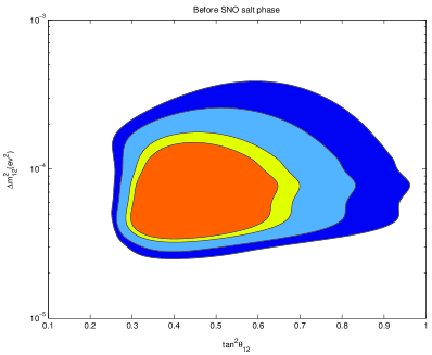
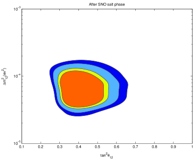
Figure 1: The 90$\%$, 95$\%$, 99$\%$, and 99.73$\%$ C.L. allowed regions in the $\Delta m_{12}^{2}-tan^{2}\theta_{12}$ plane after SNO experiments. Left corresponds to the result of SNO’s first phase, the right is the result of SNO’s salt phase case.

III Manufactured neutrinos

At present the only detected laboratory neutrinos which are sensitive to $\Delta m_{12}^{2}-\tan\theta_{12}$ parameters are reactor neutrinos. KamLAND is a first experiment to deal with these solar neutrino parameters completely from manufactured source instead of from the sun. This reactor neutrino experiment convinces scientists that the Large Mixing MSW is the solution of the solar neutrino problem [10, 12, 13].

In a reactor, anti neutrinos are released by radioactive isotope fission; the total neutrino spectrum is a rather well understood function of the thermal power $W$, the amount of thermal power $w_{i}$ emitted during the fission of a given nucleus, and the isotopic composition of the reactor fuel $f_{i}$,

$$S(E_{\nu})=\frac{W}{\sum f_{i}w_{i}}\sum f_{i}\left(\frac{dN}{dE_{\nu}}\right)_{i}$$ (3.1)

The index $i$ of $f_{i}$ stands for 4 isotopes such are ${}^{235}U$, ${}^{238}U$, ${}^{239}Pu$ and ${}^{241}Pu.$ The (dN/dE) is the energy spectrum of the fissionable isotope, it can be parameterized by the following expression[14] when $E_{\nu}\geq$ $2MeV$:

$$\frac{dN_{\nu}}{dE_{\nu}}=e^{a_{0}+a_{1}E_{\nu}+a_{2}E_{\nu}^{2}}$$ (3.2)

the coefficients $a_{i}$ depend on the nature of the fissionable isotope. KamLAND is a scintillator detector, where electronic anti neutrinos are detected by free protons via inverse $\beta-$decay reaction[14],

$$\overline{\nu}_{e}+p\rightarrow e^{+}+n$$ (3.3)

in the limit of infinite nucleon mass, the cross section of this reaction is given by $\sigma(E_{\nu})=kE_{e^{+}}P_{e^{+}}$, where $E_{e^{+}},~{}P_{e^{+}}$ are the positron energy and momentum respectively and $k$ can be taken as $k=9.55\times 10^{-44}~{}cm^{2}/MeV^{2}$. The anti neutrino events are characterized by the positron annihilation signal and the delayed neutron capture sign [6].

From the reactor to the detector, massive neutrinos oscillate on the way and change their flavor composition to a certain extent. The anti neutrino, $\overline{\nu}_{e}$, can oscillate to other flavors via $\Delta m_{12}^{2}$ and $\Delta m_{13}^{2}$. For KamLAND experiment, the distance is in the range of hundred kilometers. Due to the tiny value of $\theta_{13}$ and the value of $\Delta m_{13}^{2}$, contribution to oscillation from the biggest neutrino mass scale $m_{3}$ gives a small averaged effect thus we can reduce it to a two-flavor  neutrino analysis:

$$P(E_{\nu},L,\theta_{12},\Delta m_{12}^{2})=1-\sin^{2}(2\theta_{12})\sin^{2}\left(\frac{1.27\Delta m_{12}^{2}(\mathtt{eV}^{2})L(\mathtt{m})}{E_{\nu}(\mathtt{MeV})}\right)$$ (3.4)

The combined results of solar and reactor neutrino experimental data before ”Neutrino 2004” are shown in figs. 2.

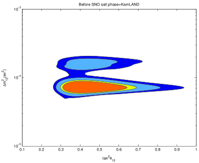
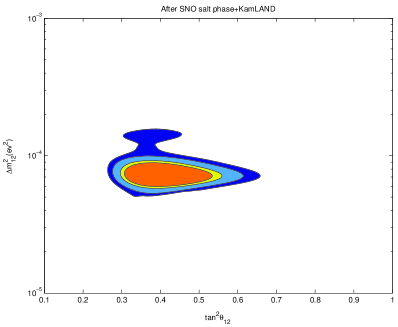
Figure 2: The combined LMA region of solar and KamLAND data before conference Nu$2004$. The difference between left and right shows improvement from SNO’s salt phase result. The confidence levels are the same as what in fig. 1.

Using the newest 766.3 Ton-Year of data published by KamLAND collaboration at conference $Neutrino$ 2004, we find the $\tan^{2}\theta_{12}-\Delta m_{12}^{2}$ allowed region with the energy spectrum in 13 bins. The result is shown in fig. 3 -left. The combined chi square is then $\chi^{2}=\chi_{\otimes}^{2}+\chi_{KL}^{2}$ with result shown in fig. 3 -right; which confirms the Large Mixing Angle MSW solution to the solar neutrino problem. The best fit point we get is

$$\tan^{2}\theta=0.4;~{}~{}~{}~{}~{}\Delta m^{2}_{21}=8.3\times 10^{-5}eV^{2},$$

which is consistent with the previous papers [15]; The day-night effect [16] for solar neutrinos is then expected to be about two to four percent.

Many other possible candidates for the solution of solar neutrino problem are excluded; sterile neutrinos are no more supported in this long-lasting puzzle. However, the most reliable candidate, the LMA MSW solution is becoming precise and more confident in terms of a much larger confidence level and much smaller allowed region. Thus we conclude that the solar neutrino problem is solved by large mixing MSW solution, with parameters shown in fig. 3.

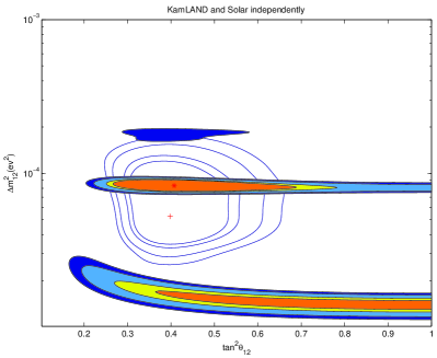
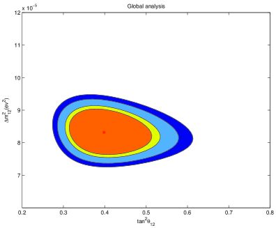
Figure 3: Left is the new KamLAND allowed regions for 766.3 Ty data, together with the LMA solution contours (not filled in) by solar neutrinos themselves. Right is the combined LMA region of solar and KamLAND data. The confidence levels are the same as what in fig. 1.

In conclusion, using the new data of KamLAND experiment we conclude that the solar neutrino solution is in the large mixing MSW adiabatic allowed region, corresponding to ($\tan^{2}\theta$, $\Delta m^{2}$) $\sim$ ($0.27-0.62$, $7.2\times 10^{-5}-9.5\times 10^{-5}eV^{2}$), at $4\sigma$ level. Which is an amazing small region in the parameter space with such a high confidence level. Our result with best fit point at ($\tan^{2}\theta$, $\Delta m^{2}$) $\sim$ ($0.4$, $8.3\times 10^{-5}eV^{2}$) is in good agreement with previous studies. Predictions of the MSW adiabatic conversion solution of the neutrino energy spectrum, the day-night effect, the seasonal variation, the ratio of CC and NC current events are all consistent with the solar data. At present, none signal indicates other solutions rather than the MSW adiabatic solution, together with the standard solar model.

Acknowledgments: One of the authors, Q.Y.L., would like to thank A. Yu. Smirnov for reading of the paper and useful suggestions, and the Abdus Salam International Center for Theoretical Physics for hospitality when the paper was written. This work is supported in part by the National Nature Science Foundation of China.

References

- [1] K. Lande, Talk given at the Neutrino ’96 Int. Conference, June 13 - 19, 1996, Helsinki, Finland (to be published in the Proceedings of the Conference); see also: R. Davis, Prog. Part. Nucl. Phys. 32, 13 (1994); B. T. Cleveland et al., Nucl. Phys. B (Proc. Suppl.) 38, 47 (1995).
- [2] V. Gavrin et al. (SAGE Collaboration), Talk given at the Neutrino ’96 Int. Conference, June 13 - 19, 1996, Helsinki, Finland (to be published in the Proceedings of the Conference); see also: J. N. Abdurashitov et al., Phys. Lett. B 328, 234 (1994).
- [3] P. Anselmann et al. (GALLEX Collaboration), Phys. Lett. B 357, 237 (1995) (see also: ibid. B 327, 377 (1994)).
- [4] K.S. Hirata, et al., Phys. Rev. D 44, 2241 (1991); K.S. Hirata, et al., Phys. Rev. Lett. 66, 9 (1991); Y. Fukuda et al., Phys. Rev. Lett. 77, (1996) 1683.
- [5] Q.R. Ahmad et al. [SNO Collaboration], Phys. Rev. Lett. 87, 071301 (2001); Phys. Rev. Lett. 89, 011301 (2002).
- [6] K. Eguchi , Phys. Rev. Lett. 90, 021802 (2003).
- [7] Q.Y. Liu and S.T. Petcov, Phys.Rev.D56: 7392 (1997); Q.Y. Liu, proceedings of 4th International Solar Neutrino Conference, Heidelberg, Germany, (1997) hep-ph/9708308.
- [8] Stephen J. Parke, Phys.Rev.Lett57, 1275 (1986).
- [9] E.Lisi, D.Montanino, Phys.Rev.D56, 1792 (1997).
- [10] P.C.de Holanda A.Yu.Smirnov Phys.Rev.D66, 113005 (2002) hepph/0205241.
- [11] J.N.Bahcall, M.H.Pinsonneault, Phys. Rev. Lett. 92, 121301 (2004); J.N.Bahcall, M.H.Pinsonneault, S.Basu,Astrophus.J.555, 990 (2001).
- [12] P.C. de Holanda and A. Yu. Smirnov, J. Cosmol. Astropart. Phys. 02, 001 (2003).
- [13] J. N. Bahcall, M. C. Gonzalez-Garcia and C. Pea-Garay, High Energy Phys. 02, 009 (2003).
- [14] P. Vogel and J. Engel, Phys. Rev. D 39, 3378 (1989); H. Murayama and A. Pierce, Phys.Rev. D65, 013012 (2002).
- [15] [KamLAND Collaboration], hep-ex/0406035; J.N. Bahcall, M.C. Gonzale-Garcia, C. Pena-Garay, hep-ph/0406294; Abhijit Bandyopadhyay, Sandhya Choubey, Srubabati Goswami, S.T. Petcov, D.P. Roy, hep-ph/0406328.
- [16] Q.Y. Liu, M. Maris and S.T. Petcov, Phys.Rev.D56, 5991 (1997); A. Dighe, Q.Y. Liu and A. Yu. Smirnov, hep-ph/9903329.