Extensive study of phase diagram for charge neutral homogeneous quark matter affected by dynamical chiral condensation
– unified picture for thermal unpairing transitions from weak to strong coupling –

Abstract

We study the phase structures of charge neutral quark matter under the $\beta$-equilibrium for a wide range of the quark-quark coupling strength within a four-Fermion model. A comprehensive and unified picture for the phase transitions from weak to strong coupling is presented. We first develop a technique to deal with the gap equation and neutrality constraints without recourse to numerical derivatives, and show that the off-diagonal color densities automatically vanish with the standard assumption for the diquark condensates. The following are shown by the numerical analyses: (i) The thermally-robustest pairing phase is the two-flavor pairing (2SC) in any coupling case, while the second one for relatively low density is the up-quark pairing (uSC) phase or the color-flavor locked (CFL) phase depending on the coupling strength and the value of strange quark mass. (ii) If the diquark coupling strength is large enough, the phase diagram is much simplified and is free from the instability problems associated with imaginary Meissner masses in the gapless phases. (iii) The interplay between the chiral and diquark dynamics may bring a non-trivial first order transition even in the pairing phases at high density. We confirm (i) also by using the Ginzburg-Landau analysis expanding the pair susceptibilities up to quartic order in the strange quark mass. We obtain the analytic expression for the doubly critical density where the two lines for the second order phase transitions merge, and below which the down-quark pairing (dSC) phase is taken over by the uSC phase. Also we study how the phase transitions from fully gapped states to partially ungapped states are smeared at finite temperature by introducing the order parameters for these transitions.

I Introduction

Surprisingly rich phase structure of quark matter is being revealed by extensive theoretical studies Bailin:1983bm ; Iwasaki:1994ij ; reviews . On the basis of the asymptotic-free nature of QCD and the attraction between quarks due to a gluon exchange, it is now believed that the ground state of the sufficiently cold and extremely dense matter is in the color-flavor locked (CFL) phase where all the quark species equally participate in pairing Alford:1998mk . In contrast, it remains still controversial what phase sets in next to the CFL as the density is decreased and/or the temperature is raised.

At zero temperature ($T=0$), the following two ingredients play crucial roles for determining the second densest phase in QCD; (i) the strange quark mass Alford:1999pa ; Schafer:1999pb ; Abuki:2003ut , and (ii) the charge neutrality constraints as well as the $\beta$-equilibrium condition Iida:2000ha ; Rajagopal:2000ff ; Alford:2002kj . The former tends to bring a Fermi-momentum mismatch between the light and strange quarks, while the latter in the paired phase tends to match the Fermi-momenta by tuning the charge chemical potentials. Some theoretical studies suggest that, when the baryon density is decreased, the effect (ii) in the CFL phase cancels the effect (i) down to some critical density, at which the CFL phase turns into the gapless CFL (gCFL) phase Alford:2003fq . In the realistic quark matter in compact stars, the effect of (ii) gives so strong constraint because of a long range nature of gauge interactions that such an exotic phase may exist stably. The gCFL phase has been extensively studied and claimed to be the most promising candidate of next phase down in density at vanishing temperature Alford:2003fq and is also known to lead an interesting astrophysical consequence on the cooling history of an aged compact star Alford:2004zr . It should be, however, noted here that the gapless phases are usually accompanied by some transverse gluonic modes with imaginary Meissner mass at low temperature Unstable ; Fukushima:2005cm , indicating the existence of more stable exotic states Reddy:2004my ; Huang:2005pv ; Casalbuoni:2005zp ; Giannakis:2005sa ; Hong:2005jv ; Gorbar:2005rx ; Schafer:2005ym . Although the resolution of the instability or finding the possible new stable state is now one of the central issues in this field, we won’t deal with this problem; nevertheless we will give some suggestions to possible resolution on the basis of the results obtained in this work.

The neutrality constraints are also known to bring about an interesting phase even at finite temperature $(T\neq 0)$. In fact, a Ginzburg-Landau analysis shows that the $d$ quark pairing phase with the $u$-$d$ and $d$-$s$ pairings, denoted by “dSC”, appears as the second phase when the 2SC (CFL) phase is cooled (heated) Iida:2003cc . The existence of such a kind of intermediate phase has also been confirmed using the NJL model Fukushima:2004zq . Also the gapless version of the dSC with an additional gapless mode is also examined for finite temperature Iida:2003cc and for zero temperature Abuki:2004zk ; the gapless dSC is shown to be always a metastable at zero temperature, while it may exist stably for nonzero temperature. It should be noted, however, that the gapless phase for nonzero temperature cannot be thermodynamically distinguished from the fully gapped one; in fact, it has no distinct phase boundary with the gapped one, and thus is of less physical interest than that at zero temperature.

In the most of the literature concerning the pairing phases of the quark matter Alford:2003fq ; Fukushima:2004zq ; Ruster:2004eg , the strange quark mass is treated as a parameter just like an external magnetic field applied to a metallic superconductor Sarma . In QCD, however, the strong attraction exists in the scaler quark-antiquark channel which leads to a non-perturbative phenomenon called the dynamical chiral condensation in the low density regime. It is interesting to investigate how the incorporation of the dynamical formation of the chiral condensates affects color superconducting phases abuki00 ; Kitazawa:2002bc . The competition between the chiral and diquark condensations under the charge neutrality constraints was first investigated in a four-Fermion model Abuki:2004zk ; it was shown that the second densest phase next to the CFL strongly depends on the quark-quark (diquark) coupling strength, and in particular, the gapless CFL phase may be washed out from the phase diagram except for an extremely weak coupling case. Their investigation is extended to finite temperatures Ruster:2005jc ; Blaschke:2005uj and recently also applied to the system with finite neutrino density Ruster:2005ib . Some of the results obtained in Ruster:2005jc ; Blaschke:2005uj , however, seemingly contradict with the previous claim by the authors of Iida:2003cc ; Fukushima:2004zq on the appearance of the dSC phase. This is one of puzzles indicating that a further investigation is needed for a systematic understanding of the phases of quark matter and transitions among them.

A main aim of this paper is to explore the phase diagram for a wide range of diquark coupling systematically and thereby give a unified picture for the phase transitions from weak to strong coupling. We clarify the detailed mechanism and features of thermal phase transitions, and make clear the relations among the previous studies Iida:2003cc ; Fukushima:2004zq ; Ruster:2005jc ; Blaschke:2005uj . In particular, we shall study the the following. (i) How the $(\mu,T)$-domain accommodating the pairing grows and that for the gapless phases vanishes as the coupling in the scaler diquark channel is increased. (ii) How we can draw a unified picture for the thermal unpairing phase transitions from weak to strong coupling; for this purpose, we extend the previous study Iida:2003cc by making re-analysis of Ginzburg-Landau expansion focusing on the effects of the terms quartic in the strange quark mass. (iii) How and why non-trivial first order phase transitions could be caused by the competition between the pairing and chiral dynamics in the strange quark sector. (iv) How the transition from the fully gapped phase to the partially ungapped (gapless) one is smeared at finite temperature by introducing a definite order parameter.

The paper is organized as follows. In Sec. II, we introduce the model and derive the gap equation under the neutrality constraints. Some technical developments are presented, by which the numerical derivatives can be replaced by simple algebraic equations. In Sec. III, we discuss the points listed above based on the numerical results. Also the Ginzburg-Landau analysis is performed and some interesting aspects of the thermal phase transitions are given at the end of this section. The summary and outlook are provided in Sec. IV. In Appendix A, we derive the Ginzburg-Landau potential expanded up to quartic order in the strange quark mass. In Appendix B, we show that the off-diagonal color densities automatically vanish under the standard ansatz for the diquark condensates.

II Formulation

In this section, we introduce our model and formulate the mean field approximation under the kinetic constraints. In Sec. II.2, we present some useful algebraic techniques to solve the gap equation and constraints without recourse to numerical derivatives.

II.1 Model

We start with the following Lagrangian as in Abuki:2004zk

$${\mathcal{L}} = \bar{q}(i\hbox to5.30904pt{\hbox to0.0pt{\hbox to5.30904pt{\hss/\hss}\hss}\hbox{$\partial$}}-\mbox{\boldmath$m$}_{0}+\mbox{\boldmath$\mu$}\gamma_{0})q+\frac{G_{d}}{16}\sum_{\eta=1}^{3}\big{[}(\bar{q}P_{\eta}^{t}\bar{q})(^{t}q\bar{P}_{\eta}q)\big{]}$$ (1)

$$+\frac{G_{s}}{8N_{c}}\big{[}(\bar{q}\mbox{\boldmath$\lambda$}_{F}q)^{2}+(\bar{q}i\gamma_{5}\mbox{\boldmath$\lambda$}_{F}q)^{2}\big{]}.$$

Here, $\mbox{\boldmath$\lambda$}_{F}=\{\sqrt{2/3}\mbox{\boldmath$1$},\vec{\lambda}_{F}\}$ are the unit matrix and the Gell-Mann matrices in the flavor space. $P_{\eta}$ is defined as Alford:2003fq

$$(P_{\eta})^{ab}_{ij}=i\gamma_{5}C\epsilon^{\eta ab}\epsilon_{\eta ij}\quad\mbox{no sum over index $\eta$}\,$$ (2)

and $\bar{P}_{\eta}=\gamma_{0}(P_{\eta})^{\dagger}\gamma_{0}$. $a,b,\cdots$ and $i,j,\cdots$ represent the color and flavor indices, respectively. The second term in Eq. (1) simulates the attractive interaction in the color anti-triplet, flavor anti-triplet and $J^{P}=0^{+}$ channel in QCD. $\mbox{\boldmath$m$}_{0}={\rm diag.}\{m_{u},m_{d},m_{s}\}$ is the current-quark mass matrix. In order to impose the color and electric neutralities, we have introduced in Eq. (1) the chemical potential matrix $\mu$ in the color-flavor space as

$$\begin{array}[]{rcl}\mbox{\boldmath$\mu$}_{ij}^{ab}&=&\displaystyle\mu-\mu_{e}Q_{ij}+\mu_{3}T_{3}^{ab}+\mu_{8}T_{8}^{ab}\\[4.30554pt] &&\displaystyle+\mu_{1}T_{1}^{ab}+\mu_{2}T_{2}^{ab}+\mu_{4}T_{4}^{ab}\\[4.30554pt] &&+\mu_{5}T_{5}^{ab}+\mu_{6}T_{6}^{ab}+\mu_{7}T_{7}^{ab}.\end{array}$$ (3)

$Q={\rm diag.}(2/3,-1/3,-1/3)$ counts electric charge of each quark species. $T_{3}={\rm diag.}(1/2,-1/2,0)$ and $T_{8}={\rm diag.}(1/3,1/3,-2/3)$ are the diagonal charges for quarks in the fundamental representation of the color SU(3). We have included the second and third lines in Eq. (3) which stand for the chemical potentials for off-diagonal color charges: It has been recently claimed that these chemical potentials should be included for the complete color neutralities Buballa:2005bv . We can prove, however, that if the diquark condensates have the color-flavor structure as given by Eq. (2), then the off-diagonal color densities must automatically vanish for $\mu_{1}=\mu_{2}=\mu_{4}=\mu_{5}=\mu_{6}=\mu_{7}=0$; see Appendix B for the detail of the proof. Thus, we can safely adopt the usual diagonal ansatz for the chemical potential matrix. The explicit forms of the diagonal elements ($\mu_{ai}=\mbox{\boldmath$\mu$}^{aa}_{ii}$) are as follows.

$$\begin{array}[]{rcl}\mu_{ru}&=&\mu-{\textstyle\frac{2}{3}}\mu_{e}+{\textstyle\frac{1}{2}}\mu_{3}+{\textstyle\frac{1}{3}}\mu_{8},\\[4.30554pt] \mu_{gd}&=&\mu+{\textstyle\frac{1}{3}}\mu_{e}-{\textstyle\frac{1}{2}}\mu_{3}+{\textstyle\frac{1}{3}}\mu_{8},\\[4.30554pt] \mu_{bs}&=&\mu+{\textstyle\frac{1}{3}}\mu_{e}-{\textstyle\frac{2}{3}}\mu_{8},\\[12.91663pt] \mu_{rd}&=&\mu+{\textstyle\frac{1}{3}}\mu_{e}+{\textstyle\frac{1}{2}}\mu_{3}+{\textstyle\frac{1}{3}}\mu_{8},\\[4.30554pt] \mu_{gu}&=&\mu-{\textstyle\frac{2}{3}}\mu_{e}-{\textstyle\frac{1}{2}}\mu_{3}+{\textstyle\frac{1}{3}}\mu_{8},\\[12.91663pt] \mu_{rs}&=&\mu+{\textstyle\frac{1}{3}}\mu_{e}+{\textstyle\frac{1}{2}}\mu_{3}+{\textstyle\frac{1}{3}}\mu_{8},\\[4.30554pt] \mu_{bu}&=&\mu-{\textstyle\frac{2}{3}}\mu_{e}-{\textstyle\frac{2}{3}}\mu_{8},\\[12.91663pt] \mu_{gs}&=&\mu+{\textstyle\frac{1}{3}}\mu_{e}-{\textstyle\frac{1}{2}}\mu_{3}+{\textstyle\frac{1}{3}}\mu_{8},\\[4.30554pt] \mu_{bd}&=&\mu+{\textstyle\frac{1}{3}}\mu_{e}-{\textstyle\frac{2}{3}}\mu_{8}\ .\\[4.30554pt] \end{array}$$ (4)

We treat the diquark coupling constant $G_{d}$ as a simple parameter, although the perturbative one-gluon exchange vertex ${\cal L}_{\rm int}=-(g^{2}/2)\bar{q}\gamma_{\mu}(\lambda_{a}/2)q\bar{q}\gamma^{\mu}(\lambda_{a}/2)q$, which is valid at extremely high density, tells us that $G_{d}/G_{s}=1/2$ with $N_{c}=3$ Steiner:2002gx ; Buballa:2001gj ; Buballa:2003qv . As a measure of coupling constant $G_{d}$, we shall mainly use the gap energy ($\Delta_{0}$) in the pure CFL phase at $\mu=500\,{\rm MeV}$ and $T=0$ in the chiral SU(3) limit, as in Alford:2003fq ; Fukushima:2004zq ; Abuki:2004zk .

We evaluate the thermodynamic potential in the mean-field approximation;

$$\begin{array}[]{rcl}\Omega&=&\Omega_{q}+\Omega_{e},\\[8.61108pt] \Omega_{q}&=&\displaystyle\frac{4}{G_{d}}\sum_{\eta=1}^{3}\Delta_{\eta}^{2}+\frac{N_{c}}{G_{s}}\sum_{i=1}^{3}(M_{i}-m_{i})^{2}\\[8.61108pt] &&\displaystyle-\frac{T}{2}\sum_{n}\int\frac{d\mbox{\boldmath$p$}}{(2\pi)^{3}}\mbox{tr}{\rm Log}\left[S^{-1}(i\omega_{n},\mbox{\boldmath$p$})\right],\\[4.30554pt] \end{array}$$ (5)

where

$$\Delta_{\eta} = \frac{G_{d}}{8}\langle^{t}qP_{\eta}q\rangle,$$ (6)

$$M = \left(\begin{array}[]{ccc}M_{u}&0&0\\ 0&M_{d}&0\\ 0&0&M_{s}\end{array}\right)$$ (10)

$$= \mbox{\boldmath$m$}_{0}-\frac{G_{s}}{2N_{c}}\left(\begin{array}[]{ccc}\langle\bar{u}u\rangle&0&0\\ 0&\langle\bar{d}d\rangle&0\\ 0&0&\langle\bar{s}s\rangle\end{array}\right),$$ (14)

are the gap parameter and constituent quark mass matrices. $S$ denotes the $72\times 72$ Nambu-Gor’kov propagator defined by

$$S^{-1}(i\omega_{n},p)=\left(\begin{array}[]{cc}\hbox to5.03125pt{\hbox to0.0pt{\hbox to5.03125pt{\hss/\hss}\hss}\hbox{$p$}}+{\mbox{\boldmath$\mu$}}\gamma_{0}-\mbox{\boldmath$M$}&\sum_{\eta}P_{\eta}\Delta_{\eta}\\ \sum_{\eta}\bar{P}_{\eta}\Delta_{\eta}&{}^{t}\hbox to5.03125pt{\hbox to0.0pt{\hbox to5.03125pt{\hss/\hss}\hss}\hbox{$p$}}-{\mbox{\boldmath$\mu$}}\gamma_{0}+\mbox{\boldmath$M$}\end{array}\right),$$ (15)

with $\hbox to5.03125pt{\hbox to0.0pt{\hbox to5.03125pt{\hss/\hss}\hss}\hbox{$p$}}=i\omega_{n}\gamma_{0}-\mbox{\boldmath$p$}\cdot\mbox{\boldmath$\gamma$}$. Finally, $\Omega_{e}$ is the contribution from massless electrons

$$\Omega_{e} = -\frac{\mu_{e}^{4}}{12\pi^{2}}-\frac{\mu_{e}^{2}T^{2}}{6}-\frac{7\pi^{2}T^{4}}{180}.$$ (16)

The optimal values of the variational parameters $\Delta_{\eta}$, $M$ and $M_{s}$ must satisfy the stationary condition (the gap equations);

$$\frac{\partial\Omega}{\partial\Delta_{\eta}}=0,\,\,\frac{\partial\Omega}{\partial M_{u,d}}=0\,\,\mbox{and}\,\,\frac{\partial\Omega}{\partial M_{s}}=0.$$ (17)

Our task is to search the minimum of the effective potential by solving these gap equations under the local electric and color charge neutrality conditions;

$$\frac{\partial\Omega}{\partial\mu_{e}}=0,\,\,\frac{\partial\Omega}{\partial\mu_{3}}=0\,\,\mbox{and}\,\,\frac{\partial\Omega}{\partial\mu_{8}}=0.$$ (18)

For a later convenience, we define here the electron density by

$$n_{e}=-\frac{\partial\Omega_{e}}{\partial\mu_{e}}=\frac{\mu_{e}^{3}}{3\pi^{2}}+\frac{\mu_{e}T^{2}}{3}.$$ (19)

The formulation made above is a straightforward extension of our previous work Abuki:2004zk to the $(T\neq 0)$ case Ruster:2005jc ; Blaschke:2005uj .

II.2 Representation of gap equation and kinetic constraints in terms of quasi-quark wave functions

In this section, we present some analytical way to deal with the gap equation and neutrality constraints. We shall show that the gap equation and neutrality constraints derived above can be further simplified with the aid of the quasi-quark wave functions (spinors). By doing this, not only the physical meanings of these equations become transparent, but also the numerical derivatives can be circumvented. In particular, the latter has a practical advantage because the computations of matrix elements are more favorable than the numerical derivatives.

First, we introduce the Nambu-Gor’kov mean field Hamiltonian density ${\mathcal{H}}(\mbox{\boldmath$p$};\mbox{\boldmath$\mu$},\mbox{\boldmath$\Delta$},\mbox{\boldmath$M$})$ following Alford:2003fq ; Fukushima:2004zq ,

$$\Gamma_{0}S^{-1}(i\omega_{n},\mbox{\boldmath$p$})\bar{\Gamma}_{0}=i\omega_{n}{\bf 1}_{72}-{\mathcal{H}}(\mbox{\boldmath$p$};\mbox{\boldmath$\mu$},\mbox{\boldmath$\Delta$},\mbox{\boldmath$M$}).$$ (20)

Here we have defined

$$\Gamma_{0}=\left(\begin{array}[]{cc}\gamma_{0}\otimes{\bf 1}_{9}&{\bf 0}\\ {\bf 0}&{\bf 1}_{36}\\ \end{array}\right),\quad\bar{\Gamma}_{0}=\left(\begin{array}[]{cc}{\bf 1}_{36}&{\bf 0}\\ {\bf 0}&\gamma_{0}\otimes{\bf 1}_{9}\\ \end{array}\right).$$ (21)

${\bf 1}_{72}$ denotes the $72$-dimensional unit matrix and ${\mathcal{H}}$ is Hamiltonian density which is also $72\times 72$ matrix in the color, flavor and spinor space. In the same manner as shown in Ruster:2005jc , we can lift the spin degeneracy away from ${\mathcal{H}}$ as ${\mathcal{H}}={\mathcal{H}}_{36}(p)\otimes P_{+}\oplus{\mathcal{H}}_{36}(-p)\otimes P_{-}$ with $P_{\pm}\equiv\frac{1\pm\hat{p}\cdot\mathstrut\mbox{\scriptsize{\boldmath$\sigma$}}\mathstrut}{2}$ being the helicity projectors. ${\mathcal{H}}_{36}(p)$ has a block-diagnalized form like ${\mathcal{H}}_{36}(p)={\mathcal{H}}_{12}^{(ur,dg,sb)}\oplus{\mathcal{H}}_{8}^{(bd,sg)}\oplus{\mathcal{H}}_{8}^{(sr,ub)}\oplus{\mathcal{H}}_{8}^{(ug,dr)}$. Furthermore, the Nambu-Gor’kov degeneracy is manifest in the latter three blocks; ${\mathcal{H}}_{8}^{(\alpha,\beta)}={\mathcal{H}}_{4}^{(\alpha,\beta)}\oplus\big{[}-{\mathcal{H}}_{4}^{(\alpha,\beta)}\big{]}$. Thus we need to know only two matrix structures of ${\mathcal{H}}_{4}^{(\alpha,\beta)}\equiv{\mathcal{H}}_{4}^{\alpha\beta}$ and ${\mathcal{H}}_{12}^{(ur,dg,sb)}\equiv{\mathcal{H}}_{12}^{uds}$ for the evaluation of the effective potential. We give the explicit form of these matrices below,

$${\mathcal{H}}^{\alpha\beta}_{4}=\left(\begin{array}[]{cccc}M_{\alpha}-\mu_{\alpha}&p&0&-i\Delta^{\alpha\beta}\\ p&-M_{\alpha}-\mu_{\alpha}&-i\Delta^{\alpha\beta}&0\\ 0&i\Delta^{\alpha\beta}&M_{\beta}+\mu_{\beta}&-p\\ i\Delta^{\alpha\beta}&0&-p&-M_{\beta}+\mu_{\beta}\end{array}\right),$$ (22)

where $\Delta^{\alpha\beta}=\Delta_{1},\Delta_{2}$ and $\Delta_{3}$ for $(\alpha,\beta)=(bd,sg),(sr,ub)$ and $(ug,dr)$, respectively, and

$${\mathcal{H}}^{uds}_{12}=\small\left(\begin{array}[]{cccccccccccc}\!\!\!M_{u}\!-\!\mu_{ur}\!\!\!\!&p&0&0&0&0&0&-i\Delta_{3}&0&0&0&-i\Delta_{2}\\ p&\!\!\!\!-M_{u}\!-\!\mu_{ur}\!\!\!\!&0&0&0&0&-i\Delta_{3}&0&0&0&-i\Delta_{2}&0\\ 0&0&\!\!\!\!M_{u}\!+\!\mu_{ur}\!\!\!\!&-p&0&i\Delta_{3}&0&0&0&i\Delta_{2}&0&0\\ 0&0&-p&\!\!\!\!-M_{u}\!+\!\mu_{ur}\!\!\!\!&i\Delta_{3}&0&0&0&i\Delta_{2}&0&0&0\\ 0&0&0&-i\Delta_{3}&\!\!\!\!M_{d}\!-\!\mu_{dg}\!\!\!\!&p&0&0&0&0&0&-i\Delta_{1}\\ 0&0&-i\Delta_{3}&0&p&\!\!\!\!-M_{d}\!-\!\mu_{dg}\!\!\!\!&0&0&0&0&-i\Delta_{1}&0\\ 0&i\Delta_{3}&0&0&0&0&\!\!\!\!M_{d}\!+\!\mu_{dg}\!\!\!\!&-p&0&i\Delta_{1}&0&0\\ i\Delta_{3}&0&0&0&0&0&-p&\!\!\!\!-M_{d}\!+\!\mu_{dg}\!\!\!\!&i\Delta_{1}&0&0&0\\ 0&0&0&-i\Delta_{2}&0&0&0&-i\Delta_{1}&\!\!\!\!M_{s}\!-\!\mu_{sb}\!\!\!\!&p&0&0\\ 0&0&-i\Delta_{2}&0&0&0&-i\Delta_{1}&0&p&\!\!\!\!-M_{s}\!-\!\mu_{sb}\!\!\!\!&0&0\\ 0&i\Delta_{2}&0&0&0&i\Delta_{1}&0&0&0&0&\!\!\!\!M_{s}\!+\!\mu_{sb}\!\!\!\!&-p\\ i\Delta_{2}&0&0&0&i\Delta_{1}&0&0&0&0&0&-p&\!\!\!\!-{M_{s}}\!+\!\mu_{sb}\!\!\!\\ \end{array}\right).$$ (23)

Because the Nambu-Gor’kov degeneracy is not removed, the eigenvalues of this matrix have six sets of the doublet $(\epsilon,-\epsilon)$ corresponding to the energies for a quasi-quark and its Nambu-Gor’kov partner (anti-quasi-quark).

Let us write $18(=72\div 2\div 2)$ independent eigenvalues of ${\mathcal{H}}$ as $\{\epsilon_{\alpha}\}$ with the index $\alpha$ redefined to the label for the quasi-quarks ($\alpha=1,2,\cdots,18$) from that for the direct products of color and flavor ($\alpha=ur,dg,sb,db,sg,sr,ub,ug,dr$). Then the thermodynamic potential can be simplified to

$$\Omega_{q} = \frac{4}{G_{d}}\sum\Delta_{\eta}^{2}+\frac{N_{c}}{G_{s}}\sum(M_{i}-m_{i})^{2}$$

$$-2\sum_{\alpha=1}^{18}\int\frac{d\mbox{\boldmath$p$}}{(2\pi)^{3}}\left[\frac{|\epsilon_{\alpha}|}{2}+T\log\left(1+e^{-|\epsilon_{\alpha}|/T}\right)\right]$$

$$+2\sum_{\alpha=1}^{18}\int\frac{d\mbox{\boldmath$p$}}{(2\pi)^{3}}\frac{p}{2}.$$

We have subtracted the vacuum contribution in the system with the nine massless quarks. It is difficult to numerically search the minima with respecting the neutrality constraints from this effective potential alone. Therefore, we search them with the aid of the gap equation which is the $\Delta$-derivative of the effective potential. If possible, numerical derivatives should be avoided because the numerical errors associated with them are not well controllable. To avoid them, we express the gap equations in terms of the eigenvectors (eigen-spinors) of ${\mathcal{H}}$. First, we simply differentiate Eq. (5) with respect to $\Delta_{\eta}$ and equating the result to zero to obtain,

$$\frac{8}{G_{d}}\Delta_{\eta}=-T\sum_{n}\int\frac{d\mbox{\boldmath$p$}}{(2\pi)^{3}}\mbox{tr}\left[\frac{1}{i\omega_{n}{\bf 1}_{36}-{\mathcal{H}}_{36}}\frac{\partial{\mathcal{H}}_{36}}{\partial\Delta_{\eta}}\right].$$ (24)

Here ${\mathcal{H}}_{36}$ is the reduced Nambu-Gor’kov Hamiltonian density defined by removing the spin degeneracy from ${\mathcal{H}}$ as was introduced above. Also we note that the reduced Hamiltonian density takes the form

$$\begin{array}[]{rcl}{\mathcal{H}}_{36}&=&{\mathcal{H}}_{0}+M_{u}\mbox{\boldmath$\phi$}_{M_{u}}+M_{d}\mbox{\boldmath$\phi$}_{M_{d}}+M_{s}\mbox{\boldmath$\phi$}_{M_{s}}\\[4.30554pt] &&+\Delta_{1}\mbox{\boldmath$\phi$}_{1}+\Delta_{2}\mbox{\boldmath$\phi$}_{2}+\Delta_{3}\mbox{\boldmath$\phi$}_{3}\\[4.30554pt] &&-3\mu\mbox{\boldmath$B$}-\mu_{e}\mbox{\boldmath$Q$}_{e}-\mu_{3}\mbox{\boldmath$T$}_{3}-\mu_{8}\mbox{\boldmath$T$}_{8},\end{array}$$ (25)

with ${\mathcal{H}}_{0}={\mathcal{H}}_{36}|_{\mathstrut\mbox{\scriptsize{\boldmath$\mu$}}\mathstrut=\mathstrut\mbox{\scriptsize{\boldmath$0$}}\mathstrut,\mathstrut\mbox{\scriptsize{\boldmath$\Delta$}}\mathstrut=\mathstrut\mbox{\scriptsize{\boldmath$0$}}\mathstrut,\mathstrut\mbox{\scriptsize{\boldmath$M$}}\mathstrut=\mathstrut\mbox{\scriptsize{\boldmath$0$}}\mathstrut}$ being the Hamiltonian density for the system with nine free massless quarks. $\mbox{\boldmath$\phi$}_{M_{i}},\mbox{\boldmath$\phi$}_{\Delta_{\eta}}$ and $\mbox{\boldmath$B$},\mbox{\boldmath$Q$}_{e},\mbox{\boldmath$T$}_{3,8}$ are the $36\times 36$ matrices with constant matrix elements. These matrices can be obtained by differentiating the reduced Hamiltonian matrix with respect to $M_{u,d},\,M_{s},\,\Delta_{1,2,3},\,\mu,\,\mu_{e,3,8}$ as follows.

$$\begin{array}[]{l}\mbox{\boldmath$\phi$}_{M_{u,d}}=\frac{\partial{\mathcal{H}}_{36}}{\partial M_{u,d}},\quad\mbox{\boldmath$\phi$}_{M_{s}}=\frac{\partial{\mathcal{H}}_{36}}{\partial M_{s}},\\[4.30554pt] \mbox{\boldmath$\phi$}_{1}=\frac{\partial{\mathcal{H}}_{36}}{\partial\Delta_{1}},\quad\mbox{\boldmath$\phi$}_{2}=\frac{\partial{\mathcal{H}}_{36}}{\partial\Delta_{2}},\quad\mbox{\boldmath$\phi$}_{3}=\frac{\partial{\mathcal{H}}_{36}}{\partial\Delta_{3}},\\[4.30554pt] \mbox{\boldmath$B$}=-\frac{1}{3}\frac{\partial{\mathcal{H}}_{36}}{\partial\mu},\quad\mbox{\boldmath$Q$}_{e}=-\frac{\partial{\mathcal{H}}_{36}}{\partial\mu_{e}},\\[4.30554pt] \mbox{\boldmath$T$}_{3}=-\frac{\partial{\mathcal{H}}_{36}}{\partial\mu_{3}},\quad\mbox{\boldmath$T$}_{8}=-\frac{\partial{\mathcal{H}}_{36}}{\partial\mu_{8}}.\\[4.30554pt] \end{array}$$ (26)

Because ${\mathcal{H}}_{36}$ is an Hermitian matrix for any momentum, we can define the complete set of spinors $\{|p,\alpha,\pm\rangle\}$ by the eigenvalue equation

$${\mathcal{H}}_{36}|p,\alpha,\pm\rangle=\pm\epsilon_{\alpha}(p)|p,\alpha,\pm\rangle,$$ (27)

$\alpha=1,\cdots,18$ and $\pm$ denote the Nambu-Gor’kov charges. Then we have

$$\langle p,\alpha,\pm|\mbox{\boldmath$\phi$}_{\eta}|p,\alpha,\pm\rangle=\pm\frac{\partial\epsilon_{\alpha}}{\partial\Delta_{\eta}},\quad(\eta=1,2,3).$$ (28)

Thus we find that Eq. (24) is reduced to

$$\frac{8}{G_{d}}\Delta_{\eta}=\sum_{\alpha=1}^{18}\int\!\!\!\frac{d\mbox{\boldmath$p$}}{(2\pi)^{3}}\tanh\left(\frac{\epsilon_{\alpha}}{2T}\right)\langle p,\alpha,+|\mbox{\boldmath$\phi$}_{\eta}|p,\alpha,+\rangle,$$

where the Matsubara summation has been performed. In much the same way, we obtain

$$\begin{array}[]{l}\displaystyle\frac{2N_{c}}{G_{s}}(M_{i}-m_{i})\\[4.30554pt] \displaystyle\qquad\quad=\sum_{\alpha=1}^{18}\int\!\!\!\frac{d\mbox{\boldmath$p$}}{(2\pi)^{3}}\tanh\left(\frac{\epsilon_{\alpha}}{2T}\right)\langle p,\alpha,+|\mbox{\boldmath$\phi$}_{M_{i}}|p,\alpha,+\rangle.\\[4.30554pt] \end{array}$$

These formulae enable us to evaluate the gap equation solely by computing the $18$-dimensional eigen-spinors defined by Eq. (27) and some matrix elements in these bases Fredrik without recourse to numerical derivatives done in Alford:2003fq ; Fukushima:2004zq ; Ruster:2005jc .

The charge neutrality constraints can be also expressed in terms of the matrix elements in the basis composed of these eigen-spinors. A straightforward application of the above method to $\rho_{3,8}=-\partial\Omega_{q}/\partial\mu_{3,8}=0$, $\rho_{e}^{q}=-\partial\Omega_{q}/\partial\mu_{e}=-n_{e}$ and $\rho_{B}=-\frac{1}{3}\partial\Omega_{q}/\partial\mu$ leads

$$0 = \sum_{\alpha=1}^{18}\int\!\!\!\frac{d\mbox{\boldmath$p$}}{(2\pi)^{3}}\left(2f_{F}(\epsilon_{\alpha})-1\right)\langle p,\alpha,+|\mbox{\boldmath$Q$}_{3,8}|p,\alpha,+\rangle,$$

$$-n_{e} = \sum_{\alpha=1}^{18}\int\!\!\!\frac{d\mbox{\boldmath$p$}}{(2\pi)^{3}}\left(2f_{F}(\epsilon_{\alpha})-1\right)\langle p,\alpha,+|\mbox{\boldmath$Q$}_{e}|p,\alpha,+\rangle,$$

$$\rho_{B} = \sum_{\alpha=1}^{18}\int\!\!\!\frac{d\mbox{\boldmath$p$}}{(2\pi)^{3}}\left(2f_{F}(\epsilon_{\alpha})-1\right)\langle p,\alpha,+|\mbox{\boldmath$B$}|p,\alpha,+\rangle.$$

Here, the Fermi-Dirac distribution function $f_{F}(\epsilon)=1/(e^{\epsilon/T}+1)$ is introduced.

At zero temperature, $f_{F}(\epsilon)=\theta(-\epsilon)$ so that the net charge will be accumulated in the blocking region where $\epsilon<0$. For the neutrality constraints to be satisfied, there must be the opposite charge density coming from a non-quark sector or from the quark sector with the finite background charge density $\int\frac{d\mathstrut\mbox{\scriptsize{\boldmath$p$}}\mathstrut}{(2\pi)^{3}}\sum_{\alpha}\langle p,\alpha,+|\mbox{\boldmath$Q$}|p,\alpha,+\rangle\neq 0$, which are supplied by tuning the charge chemical potentials $\mu_{e},\,\mu_{3}$ and $\mu_{8}$.

For a later convenience, we introduce here a charge generator

$${\tilde{Q}}=-Q-T_{3}-\frac{1}{2}T_{8},$$ (29)

the operation of which keeps the CFL state invariant (neutral) and thus represents an unbroken $U(1)$ symmetry in the CFL phase reviews . If we choose the orthogonal basis of the broken charges $(X,Y)$ in addition to unbroken ${\tilde{Q}}$ as Alford:2002kj ,

$$\begin{array}[]{rcl}X&=&Q+T_{3}-4T_{8},\\[12.91663pt] Y&=&Q-T_{3},\\[4.30554pt] \end{array}$$

the chemical potentials for these charges become

$$\begin{array}[]{rcl}\mu_{{\tilde{Q}}}&=&-\frac{4}{9}\bigl{(}\mu_{e}+\mu_{3}+{\textstyle\frac{1}{2}}\mu_{8}\bigr{)},\\[12.91663pt] \mu_{X}&=&\frac{1}{18}(-\mu_{Q}+\mu_{3}-4\mu_{8}),\\[12.91663pt] \mu_{Y}&=&\frac{1}{2}(-\mu_{Q}-\mu_{3}).\\[4.30554pt] \end{array}$$

We find that the matrix representation of ${\tilde{Q}}$ operator in the $32$-dimensional color-flavor mixed Nambu-Gor’kov base is given by

$$\mbox{\boldmath${\tilde{Q}}$}=-\frac{\partial{\mathcal{H}}_{36}}{\partial\mu_{{\tilde{Q}}}}=-\mbox{\boldmath$Q$}_{e}-\mbox{\boldmath$T$}_{3}-\frac{1}{2}\mbox{\boldmath$T$}_{8}.$$ (30)

Because this commutes with the Nambu-Gor’kov Hamiltonian density ${\mathcal{H}}_{36}$ as it should be, the quasi-particles (eigen-spinors) have definite ${\tilde{Q}}$-charges which can be shown to be of integers $(+1,0,-1)$ reviews . It is also to be noted here, that thermodynamic potential in the quark sector $\Omega_{q}$ does not depend on $\mu_{{\tilde{Q}}}$ in the fully gapped CFL phase so that it is a ${\tilde{Q}}$-insulator Alford:2002kj . Because of this, the value of $\mu_{{\tilde{Q}}}$ in the CFL phase ($T=0$) cannot be determined by the ${\tilde{Q}}$ neutrality condition in the quark sector; it should be determined completely by the vanishing-point of very gentle slope of potential curvature coming from the electron sector ($\mu_{e}^{3}/3\pi^{2}=0$).

III Numerical Results and Discussions

	Gap and mass					Conditions	Gapless quark and $\mathstrut{\tilde{Q}}$ charge
	parameters					for	($ur$-$dg$-$sb$)	($db$-$sg$)	($ub$-$sr$)	($ug$-$dr$)
Phase	$\Delta_{1}(ds)$	$\Delta_{2}(us)$	$\Delta_{3}(ud)$	$M$	$M_{s}$	chemical potentials	$0$,  $0$,  $0$	$0$,  $0$	$+1$,$-1$	$+1$,$-1$
CFL (9)$\frac{\mathstrut}{\mathstrut}$	$\Delta_{1}$	$\Delta_{2}$	$\Delta_{3}$		$M_{s}$	[$\mu_{e}=0$]	all quark modes are fully gapped
gCFL8 (8)$\frac{\mathstrut}{\mathstrut}$	$\Delta_{1}$	$\Delta_{2}$	$\Delta_{3}$		$M_{s}$	$\delta\mu_{dbsg}+\frac{M_{s}^{2}}{4\mu}\mathrel{\mathchoice{\vbox{\offinterlineskip\halign{\hfil$\displaystyle#$\hfil\cr>\crcr\vskip 0.0pt\cr\sim\crcr}}}{\vbox{\offinterlineskip\halign{\hfil$\textstyle#$\hfil\cr>\crcr\vskip 0.0pt\cr\sim\crcr}}}{\vbox{\offinterlineskip\halign{\hfil$\scriptstyle#$\hfil\cr>\crcr\vskip 0.0pt\cr\sim\crcr}}}{\vbox{\offinterlineskip\halign{\hfil$\scriptscriptstyle#$\hfil\cr>\crcr\vskip 0.0pt\cr\sim\crcr}}}}\Delta_{1}$		$db$
gCFL (7)$\frac{\mathstrut}{\mathstrut}$	$\Delta_{1}$	$\Delta_{2}$	$\Delta_{3}$		$M_{s}$	$\delta\mu_{dbsg(ubsr)}+\frac{M_{s}^{2}}{4\mu}\mathrel{\mathchoice{\vbox{\offinterlineskip\halign{\hfil$\displaystyle#$\hfil\cr>\crcr\vskip 0.0pt\cr\sim\crcr}}}{\vbox{\offinterlineskip\halign{\hfil$\textstyle#$\hfil\cr>\crcr\vskip 0.0pt\cr\sim\crcr}}}{\vbox{\offinterlineskip\halign{\hfil$\scriptstyle#$\hfil\cr>\crcr\vskip 0.0pt\cr\sim\crcr}}}{\vbox{\offinterlineskip\halign{\hfil$\scriptscriptstyle#$\hfil\cr>\crcr\vskip 0.0pt\cr\sim\crcr}}}}\Delta_{1(2)}$		$db$	$ub$
uSC (6)$\frac{\mathstrut}{\mathstrut}$		$\Delta_{2}$	$\Delta_{3}$		$M_{s}$	[$\mu_{e}=0$]	$dg$-$sb$ (1)	($db$, $sg$)
guSC (5)$\frac{\mathstrut}{\mathstrut}$		$\Delta_{2}$	$\Delta_{3}$		$M_{s}$	$\delta\mu_{ubsr}+\frac{M_{s}^{2}}{4\mu}\mathrel{\mathchoice{\vbox{\offinterlineskip\halign{\hfil$\displaystyle#$\hfil\cr>\crcr\vskip 0.0pt\cr\sim\crcr}}}{\vbox{\offinterlineskip\halign{\hfil$\textstyle#$\hfil\cr>\crcr\vskip 0.0pt\cr\sim\crcr}}}{\vbox{\offinterlineskip\halign{\hfil$\scriptstyle#$\hfil\cr>\crcr\vskip 0.0pt\cr\sim\crcr}}}{\vbox{\offinterlineskip\halign{\hfil$\scriptscriptstyle#$\hfil\cr>\crcr\vskip 0.0pt\cr\sim\crcr}}}}\Delta_{2}$	$dg$-$sb$ (1)	($db$, $sg$)	$ub$
2SC (4)$\frac{\mathstrut}{\mathstrut}$			$\Delta_{3}$		$M_{s}$	[$\mu_{3}=0]$	$sb$	($db$, $sg$)	($ub$, $sr$)
g2SC (2)$\frac{\mathstrut}{\mathstrut}$			$\Delta_{3}$		$M_{s}$	[$\mu_{3}=0$], $\delta\mu_{dgur}=\delta\mu_{drug}>\Delta_{3}$	$dg$, $sb$	($db$, $sg$)	($ub$, $sr$)	$dr$
dSC (6)$\frac{\mathstrut}{\mathstrut}$	$\Delta_{1}$		$\Delta_{3}$		$M_{s}$		$ur$-$sb$ (1)		($ub$, $sr$)
gdSC (5)$\frac{\mathstrut}{\mathstrut}$	$\Delta_{1}$		$\Delta_{3}$		$M_{s}$	$\delta\mu_{dbsg}+\frac{M_{s}^{2}}{4\mu}\mathrel{\mathchoice{\vbox{\offinterlineskip\halign{\hfil$\displaystyle#$\hfil\cr>\crcr\vskip 0.0pt\cr\sim\crcr}}}{\vbox{\offinterlineskip\halign{\hfil$\textstyle#$\hfil\cr>\crcr\vskip 0.0pt\cr\sim\crcr}}}{\vbox{\offinterlineskip\halign{\hfil$\scriptstyle#$\hfil\cr>\crcr\vskip 0.0pt\cr\sim\crcr}}}{\vbox{\offinterlineskip\halign{\hfil$\scriptscriptstyle#$\hfil\cr>\crcr\vskip 0.0pt\cr\sim\crcr}}}}\Delta_{1}$	$ur$-$sb$ (1)	$db$	($ub$, $sr$)
2SCus (4)$\frac{\mathstrut}{\mathstrut}$		$\Delta_{2}$			$M_{s}$		$dg$	($db$, $sg$)		($ub$, $sr$)
UQM (0)$\frac{\mathstrut}{\mathstrut}$					$M_{s}$	[$\mu_{3}=\mu_{8}=0]$	all quarks are ungapped.
$\chi$SB (0)$\frac{\mathstrut}{\mathstrut}$				$M$	$M_{s}$	[$\mu_{3}=\mu_{8}=0]$	all quarks are massive.

Table 1: The nonzero gap parameters, some conditions between gaps and chemical potentials, and the gapless quarks in each phase. The figure in the parenthesis in the first column represents the number of gapped quasi-quark mode. We have defined the ($ai$-$bj$) relative chemical potential by $\mu_{aibj}\equiv(\mu_{ai}-\mu_{bj})/2$. “$dg$-$sb$ (1)” means that one of the linear combinations, the $dg$ quark and the $sb$ hole remains gapless. The equation for chemical potentials in a bracket must necessarily hold for some symmetry or kinetic reason.

In this section, we present our numerical results of the solution of the gap equations, and provide the phase diagrams in the $(\mu,T)$-plane for several values of diquark coupling $G_{d}$.

Before that, we fix our model parameters. We take the chiral SU$(2)$ limit for the $u$, $d$ current quark masses ($m_{u}=m_{d}=0$) and $m_{s}=80\,{\rm MeV}$ Abuki:2004zk . These values might slightly underestimate the effect of the current masses because $m_{u,d}(2\,{\rm GeV})=3$-$4\,{\rm MeV}$ and $m_{s}(2\,{\rm GeV})=80$-$100\,{\rm MeV}$ according to the full lattice QCD simulation AliKhan:2001tx . Also we restrict the variational space by putting $M=M_{u}=M_{d}$ for simplicity. This simplification does not matter in the chiral symmetry restored phase Ruster:2005jc ; Blaschke:2005uj .

For comparison with the previous work Ruster:2005jc , we write down the dimensionless parameters adopted in this study;

$$\begin{array}[]{c}\displaystyle m_{u,d}/\Lambda=0,\quad m_{s}/\Lambda=0.1,\\[8.61108pt] \displaystyle G_{S}\Lambda^{2}\equiv\frac{G_{s}\Lambda^{2}}{8N_{c}}=2.17.\\[4.30554pt] \end{array}$$

The value of $G_{s}$ is chosen so that the dynamical quark mass at $\mu=0$ is $400\,{\rm MeV}$ for the cutoff $\Lambda=800\,{\rm MeV}$ just for comparison with our previous work Abuki:2004zk . Note, however, that this coupling is a little larger than the value extracted in the NJL model analysis of the meson spectroscopy with instanton induced six-quark coupling Hatsuda:1994pi , i.e., $G_{S}\Lambda^{2}=1.835$ which is adopted in Ruster:2005jc . We shall perform the calculation with following five different values of the diquark coupling ($G_{D}\equiv G_{d}/16$):

• extremely weak coupling:
  $\Delta_{0}=25\,{\rm MeV}\leftrightarrow G_{D}\Lambda^{2}=0.91\,\,(G_{D}/G_{S}=0.42)$

• weak coupling:
  $\Delta_{0}=80\,{\rm MeV}\leftrightarrow G_{D}\Lambda^{2}=1.37\,\,(G_{D}/G_{S}=0.63)$

• intermediate coupling:
  $\Delta_{0}=125\,{\rm MeV}\leftrightarrow G_{D}\Lambda^{2}=1.69\,\,(G_{D}/G_{S}=0.78)$

• strong coupling:
  $\Delta_{0}=160\,{\rm MeV}\leftrightarrow G_{D}\Lambda^{2}=1.92\,\,(G_{D}/G_{S}=0.88)$

• extremely strong coupling:
  $\Delta_{0}=200\,{\rm MeV}\leftrightarrow G_{D}\Lambda^{2}=2.17\,\,(G_{D}/G_{S}=1.00)$

The values of $G_{D}/G_{S}$ for the intermediate and extremely strong coupling cases are similar to those employed in Ruster:2005jc , i.e., $G_{D}/G_{S}=3/4$ and $G_{D}/G_{S}=1$. However, the following notice is in order here. (i) Our strange quark mass $m_{s}/\Lambda=0.1$ is about one half of the value $m_{s}/\Lambda=0.23$ adopted in Ruster:2005jc . (ii) We did not included the six-quark interaction which effectively increases the scalar coupling $G_{S}$. These two differences make our case favorable to the pairing phases rather than the unpaired quark matter (UQM) phase or the chiral-symmetry broken ($\chi$SB) phase. In fact, we will see that the phase diagrams for our weak coupling and intermediate coupling cases seem more or less to correspond to those for $G_{D}/G_{S}=3/4$ and $G_{D}/G_{S}=1$ in Ruster:2005jc , respectively.

We consider the candidates of phase listed in TABLE 1 as in Abuki:2004zk in the numerical analyses below.

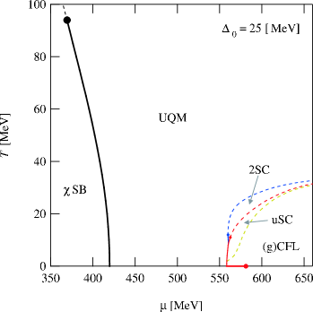
Figure 1: The phase diagram for the extremely weak coupling ($\Delta_{0}=25\,{\rm MeV}$). Sold (dashed) lines mean first (second) order transitions. Large dot placed on the $\mu$-axis ($\mu=581.1\,{\rm MeV}$) represents the transition point at which the CFL phase on the high density side continuously turns into the gCFL phase on the low density side.

III.1 Phases for extremely weak coupling

Let us first discuss the extremely weak coupling case ($\Delta_{0}=25\,{\rm MeV}$). The phase structure in this case is displayed in Fig. 1. At a first glance, we notice that the UQM phase without any symmetry breaking dominates the phase diagram pushing the superconducting phases to the high density regime. This is because the energy gain due to the $\langle\bar{s}s\rangle$ condensation in the UQM phase is larger than the paring energy under the stress as is clarified in Abuki:2004zk . There are also several thermal phase transitions. The thermally-robustest pairing phase is the 2SC and the second phase in this case is the uSC as is found in Ruster:2005jc ; Blaschke:2005uj . In the following, we shall discuss the features of these phase transitions in detail. We first make a close examination on the zero temperature case, and then investigate the finite temperature case.

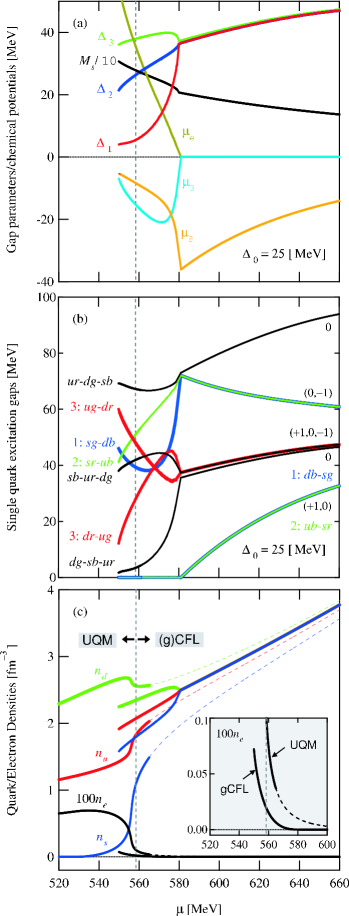
Figure 2: (a)  The (g)CFL solution of the gap equation under the neutrality constraints. The (g)CFL is energetically taken over by the UQM phase on the left side of $\mu=558.4\,{\rm MeV}$ denoted by the vertical dashed line. (b)  The excitation gaps in the nine quasi-quark spectra as a function of $\mu$. The ${\tilde{Q}}$-charge associated with each mode is also indicated. (c)  The quark and electron densities are displayed. The lines on the left hand side are densities in the UQM phase, while those on the right hand side are densities along the (g)CFL solution.

CFL/gCFL and gCFL/UQM transitions at $T=0$:

The phases realized at $T=0$ are the CFL, gCFL and UQM states. In Fig. 2(a), we show the gaps, masses, and chemical potentials along the (g)CFL solution of the gap equation. For $\mu>558.4\,{\rm MeV}$ we confirm that the condensation energy in the (g)CFL solution is largest among those for all the candidates. The excitation gaps of the nine quasi-quarks in the CFL phase are shown in FIG. 2(b). We can see from the figure that one quasi-quark has the largest excitation gap, and other quarks have relatively small gaps. The latter eight modes are the remnants of the color-flavor octet modes in the pure CFL phase at $M_{s}=0$. In the CFL phase, the non-vanishing $\mu_{8}$ and $M_{s}$ are dynamically realized so that the original symmetry of color-flavor diagonal SU$(3)_{C+V}$ is explicitly broken down to color SU$(2)_{C+V}$ (color-flavor isospin) in the Lagrangian level; because of this, the octet modes split into the isospin-singlet mode (like eta) and two set of doublet (kaonic) modes and the triplet (pionic) modes as $8\to 3\,(+1,0,-1)\,+\,2\,(+1,0)\,+\,2\,(0,-1)\,+\,1\,(0)$ where the associated ${\tilde{Q}}$-charge is indicated in the parenthesis. One of the most striking features of the CFL phase is the absence of electrons; the electric neutrality is realized solely by the quark sector $n_{u}=n_{d}=n_{s}$ as can be seen in Fig. 2(c). This CFL phase behaves as ${\tilde{Q}}$-insulator because of the absence of gapless ${\tilde{Q}}$-carriers Alford:2003fq .

As the density is decreased, the stress energy $-\mu_{8}(\mu)/2+M_{s}^{2}(\mu)/4\mu$ Alford:2003fq becomes large in the CFL state. When it reaches $\Delta_{1}=\Delta_{2}$, the first qualitative change takes place; this happens when the chemical potential is decreased down to $\mu=581.1\,{\rm MeV}$. At this point, the CFL state continuously turns into the gCFL phase. Just at the gCFL onset, the excitation gaps for the one doublet modes reaches zero as can be seen in Fig. 2(b). The situation is similar to the $K^{0}$ condensation (with a small fraction of $K^{+}$ condensation) Kaplan:1986yq ; Bedaque:2001je because the $ub$-$sr$ and $db$-$sg$ modes belong to the color-isospin SU$(2)_{C+V}$ doublet, and have ${\tilde{Q}}=+1$ and $0$, respectively.

When the chemical potential is decreased further, the gap parameters split into three different values although they are all still finite. Accordingly, the isospin SU$(2)_{C+V}$ symmetry gets broken by $\mu_{e}$ and $\mu_{3}$ so that the gaps in quasi-quark dispersions all take different values (see FIG. 2(b)). We remark that the electron chemical potential or its density actually serves as an order parameter of the CFL/gCFL (insulator/metal) transition as claimed in Alford:2003fq .

The gCFL phase continues to be the ground state down to $\mu=558.4\,{\rm MeV}$ below which the UQM phase is more favorable in terms of the thermodynamic potential. When the transition gCFL $\to$ UQM takes place, there should be the large re-configuration of the flavor contents as can be seen in FIG. 2(c). Thus, this transition requires a lot of electro-weak processes which include the $d$ production like $ug(ur)\to dg(dr)+e^{+}+\nu_{e}$ in addition to the decay to the gapless modes accompanied by the electron production $db\to ub+e^{-}+\bar{\nu}_{e}$ and the $s$ quark decay $sb+u\to db+u$. We should note that there still remains an open interesting question how the UQM droplets are dynamically formed in the gCFL phase and grow against the surface tension.

We have seen that, as the density is decreased, the CFL phase turns into the gCFL phase, and then the gCFL phase gets taken over by the UQM phase. Accordingly, the number of gapped quasi-quark modes decrease as 9 (CFL) $\to$ 7 (gCFL) $\to$ 0 (UQM) at $T=0$ as shown in the previous work Abuki:2004zk . Next, we will discuss how the situation is changed in the $T\neq 0$ case.

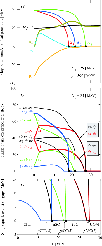
Figure 3: (a)  The gap and mass parameters, and the chemical potentials as a function of $T$ at $\mu=590\,{\rm MeV}$ so that the system at $T=0$ stays in the CFL phase (see FIG. 2). (b)  The nine quasi-quark gaps versus $T$. Nonzero ${\tilde{Q}}$-charge is also indicated by $\pm 1$. (c)  Just an enlargement of the figure (b).

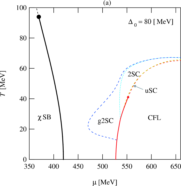
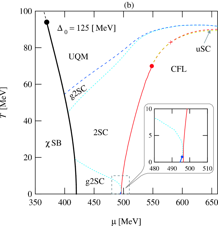
Figure 4: The phase diagram for the weak coupling $(\Delta_{0}=80\,{\rm MeV})$ (a), and for the intermediate coupling $(\Delta_{0}=125\,{\rm MeV})$ (b).

Phase transitions and crossovers for finite temperature:

We show here that the quark matter undergoes a sequence of the transitions, CFL(9) $\to$ gCFL${}_{8}(8)$ $\to$ uSC(6) $\to$ guSC(5) $\to$ 2SC(4) $\to$ g2SC(2) $\to$ UQM(0) as $T$ becomes large; the number of the gapped modes in each phase is indicated with a parenthesis.

In FIG. 3(a), we show the $T$-dependence of the gaps, masses, and chemical potentials. The figure shows that the $\Delta_{1}$ first melts and then $\Delta_{2}$ disappears as $T$ is increased. The thermally-robustest pairing is the 2SC, while second one is the uSC, which is in agreement with the result in Ruster:2005jc . This conclusion will be found to be also consistent with the Ginzburg-Landau analysis given in Sec. III.5, where we extend the previous study Iida:2003cc and see that the large value of the strange quark mass actually disfavors the dSC phase.

In order to study the thermal transition in more detail, we have also plotted the $T$-dependence of the gaps in the nine quasi-quark spectra in FIG. 3(b). FIG. 3(c) is just an enlargement of (b). The three large points on the horizontal line indicate $T=T_{c\eta}$ $(\eta=1,2,3)$ at which $\Delta_{\eta}$ vanishes (the same as the large points in FIG. 3(a)). When the temperature is increased from $T=0$, the first qualitative change occurs at $T\sim 15.8\,{\rm MeV}$ where one of the $db$-$sg$ dispersion becomes gapless and the gCFL₈ phase (gCFL in Ruster:2005ib ) sets in. Unlike the gCFL phase at $T=0$, the $ub$-$sr$ dispersion does not become gapless at this point. From the viewpoint of the insulator-to-metal transition, however, the sharp phase transition is smoothen not only due to the absence of the gapless $ub$-$sr$ mode with ${\tilde{Q}}=1$, but also to the thermally-excited on-shell quasi-quarks at finite temperature as the latter ingredient is already noticed in Fukushima:2004zq . In fact, from the FIG. 3(b), we can see that the $ub$-$sr$ (${\tilde{Q}}=+1$) mode is lighter than the $db$-$sg$ (${\tilde{Q}}=-1$) mode for $T\mathrel{\mathchoice{\vbox{\offinterlineskip\halign{\hfil$\displaystyle#$\hfil\cr<\crcr\vskip 0.0pt\cr\sim\crcr}}}{\vbox{\offinterlineskip\halign{\hfil$\textstyle#$\hfil\cr<\crcr\vskip 0.0pt\cr\sim\crcr}}}{\vbox{\offinterlineskip\halign{\hfil$\scriptstyle#$\hfil\cr<\crcr\vskip 0.0pt\cr\sim\crcr}}}{\vbox{\offinterlineskip\halign{\hfil$\scriptscriptstyle#$\hfil\cr<\crcr\vskip 0.0pt\cr\sim\crcr}}}}5\,{\rm MeV}$ and accordingly there is a little excess of the quasi-quarks with ${\tilde{Q}}=+1$ in the system. In order to achieve the neutrality, there must be the equal amount of electrons so that $\mu_{e}$ takes positive finite value as long as $T$ is finite. As a result, the CFL-gCFL₈ (insulator-metal) transition becomes a smooth crossover.

When $T$ is increased further beyond the gCFL₈ onset, $\Delta_{1}$ disappears at $T\sim 18.4\,{\rm MeV}$. This is a second order phase transition of gCFL₈ $\to$ uSC. As a consequence, two quasi-quark modes become gapless as is seen in FIG. 3(b); one is the $sg$-$db$ mode i.e., the partner of the gapless $bd$-$sg$ mode, while the other is the isospin singlet $dg$-$sb$-$ur$ mode.

Next qualitative change occurs when $T$ is increased to $T\sim 21.2\,{\rm MeV}$. At this point, the $ub$-$sr$ mode with ${\tilde{Q}}=+1$ becomes gapless and the guSC(5) phase sets in. Notice that because the thermally-excited quasi-quarks are already present in the system over the range ($E_{ub\mbox{\scriptsize-}sr}\mathrel{\mathchoice{\vbox{\offinterlineskip\halign{\hfil$\displaystyle#$\hfil\cr<\crcr\vskip 0.0pt\cr\sim\crcr}}}{\vbox{\offinterlineskip\halign{\hfil$\textstyle#$\hfil\cr<\crcr\vskip 0.0pt\cr\sim\crcr}}}{\vbox{\offinterlineskip\halign{\hfil$\scriptstyle#$\hfil\cr<\crcr\vskip 0.0pt\cr\sim\crcr}}}{\vbox{\offinterlineskip\halign{\hfil$\scriptscriptstyle#$\hfil\cr<\crcr\vskip 0.0pt\cr\sim\crcr}}}}T$), there is no sharp boundary between the uSC(6) and guSC(5) phases.

At a little higher temperature $T\sim 21.8\,{\rm MeV}$, $\Delta_{2}$ vanishes and above which the 2SC(4) phase is realized. At this transition point, the $sr$-$ub$ mode having ${\tilde{Q}}=+1$ becomes gapless. Through the gap parameter $\Delta_{2}$, this $sr$-$ub$ mode is paired with its partner, i.e., the gapless $ub$-$sr$ mode. When $\Delta_{2}\to 0$, these two modes get unpaired to become the bare $ub$ and $sr$ quarks. This guSC(5) $\to$ 2SC(4) phase transition is of second order.

As $T$ is increased further, the crossover 2SC(4) $\to$ g2SC(2) takes place at $T\sim 26.6\,{\rm MeV}$, and finally the g2SC(2) is taken over by the UQM(0) phase through a second order phase transition at $T\sim 27.4\,{\rm MeV}$.

We have found that the excitation gaps behave in a more complicated manner than the gap parameters as functions of $T$. However, as we explained, there are no sharp boundary with thermodynamical singularity between CFL(9) and gCFL₈(8), uSC(6) and guSC(5), and 2SC(4) and 2SC(2) transitions. For this reason, we did not indicate these crossover boundaries in the phase diagram of FIG. 1.

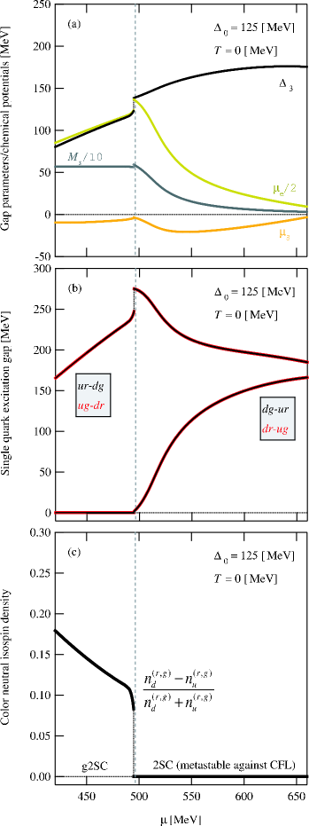
Figure 5: (a)  The gap and mass parameters, and the chemical potentials versus $\mu$ along the (g)2SC solution. The dashed line placed on $\mu=496.4\,{\rm MeV}$ represents the point above which the 2SC state is metastable against the CFL. (b)  The four quasi-quark gaps as a function of $\mu$. (c)  The fraction of the isospin density $\sum_{a=r,g}(n_{d}^{a}-n_{u}^{a})$ to the iso-scaler density $\sum_{a=r,g}(n_{u}^{a}+n_{d}^{a})$; by the summation, this quantity is made of neutral with respect to the remaining SU$(2)_{\mbox{\scriptsize color}}$ charges.

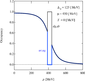
Figure 6: The occupation number for $u$ and $d$ quarks in the pairing $(r,g)$ sector as a function of momentum $p$ in the g2SC phase at $\Delta_{0}=125\,{\rm MeV}$, $\mu=450\,{\rm MeV}$ and $T=0$.

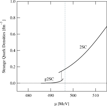
Figure 7: The strange quark density as a function of $\mu$ in the 2SC sector. The vertical dashed line is the same as that in FIG. 5. At $\mu=498.4\,{\rm MeV}$, the strange quark density jumps accompanying the first order 2SC/g2SC transition.

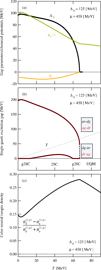
Figure 8: (a)  The gap parameter $\Delta_{3}$ and the chemical potential $\mu_{e,8}$ versus $T$ for $\Delta_{0}=125\,{\rm MeV}$ and $\mu=450\,{\rm MeV}$. (b)  The excitation gaps in the four quasi-quark spectra as a function of $T$. (c)  The SU$(2)_{\mbox{\scriptsize color}}$ neutral isospin density divided by the total isoscalar density as a function of $T$. This quantity is an order parameter for the 2SC/g2SC transition at $T=0$.

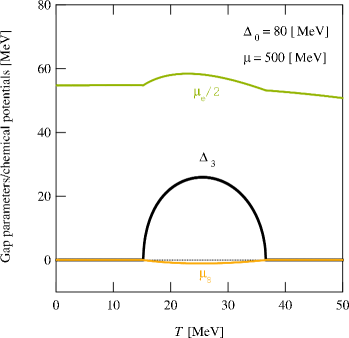
Figure 9: The gap parameter $\Delta_{3}$ and the chemical potentials $(\mu_{e}/2,\mu_{8})$ versus temperature $T$ at $\mu=500\,{\rm MeV}$ and $\Delta_{0}=80\,{\rm MeV}$; weak coupling case.

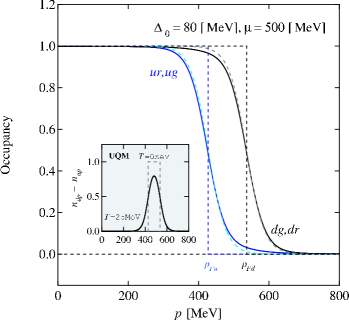
Figure 10: Solid lines are the occupation numbers for the $u$ and $d$ quarks in the g2SC phase $(\mu,T)=(500\,{\rm MeV},25\,{\rm MeV})$ as a function of momentum $p$. The sharp Fermi surfaces for the $u$ and $d$ quarks at $T=0$ are also indicated by the dashed lines. Dashed curves are the $u$ and $d$ occupancies for the unstable UQM phase at $T=25\,{\rm MeV}$. The inset is the quantity $n_{dp}^{(r,g)}-n_{dp}^{(r,g)}$, i.e., the isospin mismatch in the UQM at $T=0$ (dashed line) and for the unstable UQM at $T=25\,{\rm MeV}$ (solid line).

III.2 Phases for weak and intermediate coupling

Let us next examine the weak and intermediate coupling cases ($\Delta_{0}=80$ and $\Delta_{0}=125\,{\rm MeV}$). In FIG. 4, the phase diagrams for the both cases are shown.

III.2.1 Phases for the intermediate coupling

We first discuss the case of the intermediate coupling $\Delta_{0}=125\,{\rm MeV}$, in advance of the weak coupling case.

FIG. 4(b) shows that the UQM and gCFL phases disappear at $T=0$ and the g2SC (CFL) phase exist in the intermediate (high) density regime Abuki:2004zk . We notice that the fully gapped 2SC phase exists in a small $\mu$-region between the CFL and g2SC phases. Also we notice that the transition between the 2SC and g2SC phases is of a first order accompanied by a jump in the dynamical strange quark mass and other physical quantities. This is in contrast to the usual 2SC/g2SC transition without strange quarks. We will later discuss this point in detail.

The phases for $T\neq 0$ also differ from the extremely weak coupling case: (i) The window for the uSC phase is pushed away to higher density side and is confined in a small region. The cross placed on the dashed line represents the point at which the window for the uSC phase opens. (ii) The large dot putted on the CFL/2SC transition line indicates the critical endpoint; the dashed line between the large dot and the cross shows that there exists the continuous phase transition of 2SC $\leftrightarrow$ CFL. In the following, we shall discuss the detail of the 2SC/g2SC transitions. We first study the $T=0$ case and then investigate the $T\neq 0$ case.

2SC/g2SC transition at $T=0$:

In FIG. 5(a), we explicitly show the solution of the gap equation in the 2SC sector at $T=0$. Just to make the argument clear, we show the 2SC solution for the entire $\mu$-space, but note that the 2SC phase is metastable being energetically taken over by the CFL phase in the right hand side of the vertical dashed line placed on $\mu=496.4\,{\rm MeV}$; we should keep in mind that the window for the 2SC phase is extremely narrow. Below the critical chemical potential $\mu=494.8\,{\rm MeV}$, $(\mu_{ug}-\mu_{dr})/2=(\mu_{ur}-\mu_{dg})/2=\mu_{e}/2$ becomes greater than the gap parameter $\Delta_{3}$, and as a consequence, the fully gapped 2SC is taken over by the partially ungapped g2SC (See FIG. 5(b)). In FIG. 5(c), the ratio of the SU$(2)_{\mbox{\scriptsize color}}$ neutral isospin density $\sum_{a=r,g}(n_{d}^{a}-n_{u}^{a})$ relative to the isospin scaler density is shown as a function of $\mu$. This quantity serves as an order parameter with which the g2SC phase can be distinguished from the 2SC phase; in the fully gapped 2SC phase, this quantity must be zero because the equal number of $u$ and $d$ quarks are required for the pairing, while in the g2SC phase, the quantity becomes nonzero because of the accumulation of isospin charge in the blocking region. This is clearly seen in the plot of the occupation numbers in the g2SC phase (See FIG. 6). From all the three figures (FIG. 5) in addition to the analyses of the thermodynamic potential, we can conclude that the 2SC/g2SC transition is of first order unlike the usual case without the chiral dynamics, i.e., the $\langle\bar{s}s\rangle$ condensation.

The first order phase transition between these two phases is brought about actually by the competition between the chiral $\langle\bar{s}s\rangle$ condensation and the quark pairing dynamics in the $u$-$d$ sector as was first recognized in Abuki:2004zk . We can see a small jump in the strange quark mass at the transition point in FIG. 5(a). The strange quark mass reaches almost the vacuum value on the g2SC side, while it varies on the 2SC side and becomes smaller as the density goes high. Accordingly the strange quarks are absent in the g2SC side, while a small number of $s$ quarks are present in the 2SC side and it grows with increasing density. This is naturally understood as follows: In the fully gapped 2SC phase, the $u(rg)$ and $d(rg)$ quark densities should be equal for accommodating the $\Delta_{3}$-condensate. Because of the positive electric charge $1/3=2/3-1/3$ coming from this $SU(2)_{\mbox{\scriptsize color}}$ sector, the system needs strange quarks, electrons and $db$-quarks. Thus, the high density condition [$M_{s}\ll\mu$] favors the 2SC realization because plenty of strange quarks providing negative charges can exist in the system as can be confirmed by the plot of strange quark density in FIG. 7. But this condition is in turn disfavored with respect to the chiral condensation energy. On the other hand, the g2SC phase can realize the electric neutrality with a less number of strange quarks because of a $d$ quark excess to $u$ quarks in the $SU(2)_{\mbox{\scriptsize color}}$ sector. Accordingly the g2SC phase is not so much disfavored by the chiral $\langle\bar{s}s\rangle$ condensation ($M_{s}\mathrel{\mathchoice{\vbox{\offinterlineskip\halign{\hfil$\displaystyle#$\hfil\cr>\crcr\vskip 0.0pt\cr\sim\crcr}}}{\vbox{\offinterlineskip\halign{\hfil$\textstyle#$\hfil\cr>\crcr\vskip 0.0pt\cr\sim\crcr}}}{\vbox{\offinterlineskip\halign{\hfil$\scriptstyle#$\hfil\cr>\crcr\vskip 0.0pt\cr\sim\crcr}}}{\vbox{\offinterlineskip\halign{\hfil$\scriptscriptstyle#$\hfil\cr>\crcr\vskip 0.0pt\cr\sim\crcr}}}}\mu$) in comparison with the 2SC phase . In short, the g2SC phase can co-exist with the chiral symmetry broken phase easier than the fully gapped 2SC phase can do. The competition of these two ingredients makes the 2SC/g2SC transition be of first order at $T=0$.

g2SC/2SC/g2SC crossovers for $T\neq 0$:

We now investigate how the situation changes for the 2SC/g2SC transition at $T\neq 0$. The phase diagram displayed in FIG. 4(b) shows that, in a relatively low density regime ($430\,{\rm MeV}\mathrel{\mathchoice{\vbox{\offinterlineskip\halign{\hfil$\displaystyle#$\hfil\cr<\crcr\vskip 0.0pt\cr\sim\crcr}}}{\vbox{\offinterlineskip\halign{\hfil$\textstyle#$\hfil\cr<\crcr\vskip 0.0pt\cr\sim\crcr}}}{\vbox{\offinterlineskip\halign{\hfil$\scriptstyle#$\hfil\cr<\crcr\vskip 0.0pt\cr\sim\crcr}}}{\vbox{\offinterlineskip\halign{\hfil$\scriptscriptstyle#$\hfil\cr<\crcr\vskip 0.0pt\cr\sim\crcr}}}}\mu\mathrel{\mathchoice{\vbox{\offinterlineskip\halign{\hfil$\displaystyle#$\hfil\cr<\crcr\vskip 0.0pt\cr\sim\crcr}}}{\vbox{\offinterlineskip\halign{\hfil$\textstyle#$\hfil\cr<\crcr\vskip 0.0pt\cr\sim\crcr}}}{\vbox{\offinterlineskip\halign{\hfil$\scriptstyle#$\hfil\cr<\crcr\vskip 0.0pt\cr\sim\crcr}}}{\vbox{\offinterlineskip\halign{\hfil$\scriptscriptstyle#$\hfil\cr<\crcr\vskip 0.0pt\cr\sim\crcr}}}}480\,{\rm MeV}$), the g2SC/2SC and 2SC/g2SC transitions take place successively when the quark matter is heated. This kind of exotic situation is already found in Shovkovy:2003uu where the systematic study of the coupling strength dependence of the 2SC/g2SC transition is done within the two-flavor NJL model. In our case, the strange quark mass reaches almost its vacuum value in this region so that the pairing dynamics becomes similar to those in the previous two-flavor models. In FIG. 8, we show how the physical quantities behave through these phase transitions for $\mu=450\,{\rm MeV}$. FIG. 8(a) shows the gap parameters and the chemical potentials as a function of $T$. $\mu_{e}/2$ and $\Delta_{3}$ cross each other twice with increasing $T$ so that the system undergoes the 2SC/g2SC and g2SC/2SC transitions before the pairing is overwhelmed by the UQM. FIG. 8(b) shows the gaps in the quasi-quark spectra. We note, however, that the excitation gap in the $dg$-$ur$ ($dr$-$ug$) quasi-quark spectrum is always smaller than $T$ so that these quasi-quarks are thermally-excited irrespective of whether the system is in the 2SC phase or the g2SC phase. These quasi-quarks smear the 2SC/g2SC and g2SC/2SC transitions. Accordingly, no thermodynamic singularity is associated with these transitions except for the final g2SC-UQM ($\Delta_{3}\to 0$) transition. This can be understood also in terms of the order parameter for the 2SC/g2SC transition at $T=0$. FIG. 8(c) shows the SU$(2)_{\mbox{\scriptsize color}}$ neutral isospin density $\sum_{a=r,g}(n_{d}^{a}-n_{u}^{a})$ normalized by isoscalar density as a function of $T$. From the figure, we can see that the g2SC/2SC transitions are crossovers; the order parameter always takes nonzero value and the system is always isospin charged due to the thermally-excited quasi-quarks even for $\mu_{e}/2<\Delta_{3}$ region.

III.2.2 Phases for the weak coupling

Now we turn to the weak coupling case ($\Delta_{0}=80\,{\rm MeV}$). The phase diagram is shown in FIG. 4(a). In this case, the diquark coupling is not stronger enough to exclude the UQM phase from $T=0$, while the gCFL phase is overwhelmed by the UQM with a large $\langle\bar{s}s\rangle$ and thus is washed out as was first noted in the previous work Abuki:2004zk .

One of the most striking features in this case is the appearance of the g2SC phase for $T\neq 0$ even when the UQM phase is realized at $T=0$. This somewhat strange aspect of the color-neutral g2SC phase was first recognized in Shovkovy:2003uu and has been further confirmed in Fukushima:2004zq , although it seems that physics for this phenomenon has not yet been clarified enough. In FIG. 9, we show the gap parameter $\Delta_{3}$ and the chemical potential $(\mu_{e}/2,\mu_{8})$ as a function of $T$ in this situation ($\mu=500\,{\rm MeV}$). At $T=0$, the system is in the UQM phase, and the $\Delta_{3}$-condensate appears at $T\sim 16\,{\rm MeV}$ and then the 2SC turns again into the UQM phase at $T\sim 36.5\,{\rm MeV}$. $\mu_{e}/2$ is always larger than $\Delta_{3}$ so that the system is in the “g2SC” phase accompanied by only two gapped quasi-quarks, i.e., the $ur$-$dg$ and $ug$-$dr$ modes. However, it should be again noted here that the two phases (2SC and g2SC) are not thermodynamically distinguishable for $T\neq 0$ as explained in the previous section. To understand the appearance of the 2SC phase for $T\neq 0$, we show the occupation number of the $u$ and $d$ quarks for various situations in FIG. 10. There are sharp Fermi surfaces at $T=0$ which are indicated by dashed lines, i.e., one for $d$ quarks at $p_{Fd}=\mu+\mu_{e}^{(T=0)}/3$ and the other for $u$ quarks at $p_{Fu}=\mu-2\mu_{e}^{(T=0)}/3$. The dashed curves show the $u$ and $d$ quark occupancies at $T=25\,{\rm MeV}$ in the UQM phase which is unstable to the formation of $u$-$d$ pairs. Quarks are thermally-excited so that the distribution is somewhat smeared. We note that because of this thermal effect, the $u$ and $d$ quarks are under a better kinematical matching than the situation at $T=0$; from the inset of the figure, we can see that the isospin mismatch $(u_{d}-u_{u})$ at the averaged Fermi momentum $p=(p_{Fd}+p_{Fu})/2$ is reduced in the $T=25\,{\rm MeV}$ case from the unity, i.e., the value in the $T=0$ case. As a result, it is easier for the quark matter in the UQM phase to form the diquark condensate in the isospin singlet channel at finite temperature than at $T=0$. The solid lines show the occupation numbers after this reconfiguration takes place (the g2SC phase). We remark that unlike the occupation numbers in the g2SC phase at $T=0$ drawn in FIG. 6, there are no singular points in those for the thermally-smeared g2SC phase for $T\neq 0$.

III.3 Phases for (extremely) strong coupling

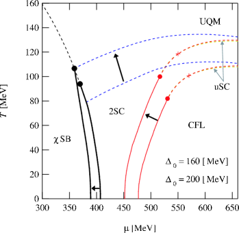
Figure 11: The phase diagrams for the strong coupling $(\Delta_{0}=160\,{\rm MeV})$ and for the extremely strong coupling $(\Delta_{0}=200\,{\rm MeV})$. Phase boundaries shift in the directions indicated by the bold arrows when the diquark coupling is increased from $\Delta_{0}=160\,{\rm MeV}$ to $\Delta_{0}=200\,{\rm MeV}$.

We next discuss the strong and extremely strong coupling cases, $\Delta_{0}=160\,{\rm MeV}$ and $200\,{\rm MeV}$, respectively. The phase diagrams are depicted in FIG. 11. The phase boundaries move in the directions indicated by the bold arrows when the diquark coupling is increased from $\Delta_{0}=160\,{\rm MeV}$ to $\Delta_{0}=200\,{\rm MeV}$. One can see that both the phase structures in these cases are qualitatively identical and are much simpler than those for the weak and intermediate couplings. The premature gapless phases disappear from the low temperature regime, and only the two major pairing phases remain in the phase diagram, i.e., the CFL phase and the 2SC phase. In each case, we still have a small window for the uSC realization as a precursory phase of the CFL $\to$ 2SC transition in the high $\mu$-region of the phase diagram. However, one should notice that the critical temperature for the 2SC/UQM transition has a maximum in this chemical potential region, which might imply that this shrinkage of the uSC window is due to a cutoff artifact. It should be also noted that when the diquark coupling is large, the 2SC phase encroaches upon the domain for the $\chi$SB phase. In addition, the 2SC/UQM transition temperature becomes larger with increasing diquark coupling, and at some critical coupling ($\Delta_{0}=\Delta_{\rm c}$), it reaches the tricritical point of the chiral phase transition: At this coupling, the chiral tricritical point acquires the nature of the doubly critical point where the two second order critical lines merge; one is for the 2SC/UQM transition and the other is for the UQM/$\chi$SB transition. Because this point has both the tricritical and doubly critical natures, we call it the “TDCP” point. When the diquark coupling is increased beyond this critical coupling $\Delta_{\rm c}$, the TDCP point shifts to higher temperature because the 2SC/$\chi$SB transition is always of first order Ruster:2005jc . Our calculation indicates the critical coupling $\Delta_{\rm c}$ where the tricritical point obtains a DCP nature lies between $\Delta_{0}=160\,{\rm MeV}$ and $\Delta_{0}=200\,{\rm MeV}$.

Finally, it is worth mentioning that the phases in the strong coupling cases discussed above are all free from the instability problem associated with the imaginary Meissner masses .

III.4 Baryon density $\rho_{B}$ at $T=0$

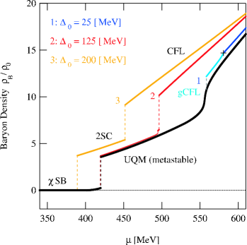
Figure 12: The baryon number density at $T=0$ in the unit of $\rho_{0}=0.17\,{\rm fm}^{-3}$, i.e., the normal nuclear density. $1$, $2$, and $3$ indicated for each line correspond to the following three cases; the extremely weak coupling ($\Delta_{0}=25\,{\rm MeV}$), the intermediate coupling ($\Delta_{0}=125\,{\rm MeV}$), and the extremely strong coupling ($\Delta_{0}=200\,{\rm MeV}$), respectively. The cross placed on the CFL line indicates the transition point at which the CFL continuously turns into the gCFL phase.

We have investigated the phase structures of the quark matter in the $(\mu,T)$-plane for several diquark couplings. It is, however, sometimes more convenient to describe the system in the $(\rho_{B},T)$-plane to have a physics intuition into the system. Also it is necessary to have the equation of state as a function of $\rho_{B}$ to clarify the inner structure of compact stars Blaschke:2005uj . Here one should notice that when multiple phases coexist at a temperature with the same chemical potentials, each phase may have a different baryon density from each other; these phases are actually realized in a mixed phase where the phases with different baryon densities coexist.

Here, we ask how dense each phase at $T=0$ is. In FIG. 12, we show the baryon density $\rho_{B}$ versus chemical potential $\mu$ at $T=0$ in the following three cases; (1) the extremely weak coupling $\Delta_{0}=25\,{\rm MeV}$, (2) the intermediate coupling $\Delta_{0}=125\,{\rm MeV}$ and (3) the extremely strong coupling $\Delta_{0}=200\,{\rm MeV}$. In any case, as the chemical potential is lowered from the highest value, the baryon density decreases and shows several jumps associated with first order transitions. We start with the case (1). In this case, the ground state at highest density, about 15 times the normal nuclear matter density, is in the CFL phase. When the density is decreased down to the point indicated by the cross, the CFL continuously turns into the gCFL phase with a steeper gradient $\frac{d\rho}{d\mu}=\frac{1}{\rho}\big{(}\frac{d\rho}{dP}\big{)}_{\scriptstyle T}\equiv\kappa_{\scriptstyle T}(\rho)$, i.e., a larger compressibility or equivalently, a larger number fluctuation (susceptibility $\chi_{\rho\rho}^{T}(r)$) attributed to gapless modes. If the density is decreased further, the first order transition from the gCFL to the UQM takes place; accordingly the baryon density drops down to almost ten times the nuclear density through a mixed phase of the two phases. The UQM phase continues down to $\sim 3$ times the nuclear density, and then gets taken over by the chiral symmetry broken phase. The situation becomes slightly complicated in the case (2). The densest phase is again the CFL. As the density is decreased, the CFL phase persists down to almost ten times the nuclear density. Then the quark system undergoes a first order phase transition to the 2SC phase via the dynamical nucleation and growth of the low density 2SC droplets in the CFL phase. This nucleation also needs a lot of weak processes. The density window accommodating the 2SC phase is extremely small and the 2SC phase gets immediately taken over by the g2SC phase. The g2SC phase finally changes into the $\chi$SB phase. Similarly in the case (3), the baryon density drops twice according to the CFL/2SC and 2SC/$\chi$SB transitions. It is interesting that the lowest baryon density of the CFL phase decreases with increasing diquark coupling while the density at the same $\mu$ is enhanced by the factor $\Delta_{0}^{2}/\mu^{2}$. It should be noted, however, that the $\rho$-$\mu$ relation will be affected by the fluctuation effect so that the density becomes even larger due to bosonic degrees of freedom in the strong coupling cases Nishida:2005ds .

III.5 The Ginzburg-Landau analysis

In this section, we make a systematic Ginzburg-Landau analysis in order to understand why the dSC phase does not appear in our calculation of the phase diagram. Our analysis is an extension of the previous work Iida:2003cc ; we expand the Ginzburg-Landau coefficients up to quartic order in $M_{s}$ which were not taken into account in Iida:2003cc but turn out to play an important role for the relatively strong coupling (low density) regime. We also notice that this extension makes it possible to provide a unified and systematic description of the thermal pairing/unpairing transitions obtained in the NJL Ruster:2005jc and the Ginzburg-Landau analysis Iida:2003cc .

If the phase transition at finite temperature is of second order where the condensate $\Delta_{\eta}$ vanishes at the critical point, we can expand the effective potential in terms of the gap parameters near the critical temperature $T_{c}$. In this section, we focus on the regime where the chiral symmetry is restored, and assume that the thermal pairing/unpairing transitions are not so much affected by the chiral dynamics there. Thus, we shall switch off the scalar coupling $G_{s}$ in our NJL lagrangian, Eq. (1), and treat the strange quark mass $M_{s}$ as a constant parameter. This is nothing but a model used in Fukushima:2004zq ; Fukushima:2005fh , which will be referred as the diquark NJL model hereafter in order to distinguish it from the present NJL model analysis with the scalar coupling, i.e., Eq. (1). Treating $M_{s}$ as a parameter can be justified by the fact that $M_{s}$ does not so much vary in the vicinity of $T_{c}$ (See FIG. 3(a)). Either from the diquark NJL model or from the QCD-like theory with the Cornwall-Jackiw-Tomboulis potential up to 2PI graphs Iida:2003cc , we can derive the Ginzburg-Landau potential. We first emphasize that each of the Ginzburg-Landau coefficients becomes a function of $M_{s}$ under the neutrality constraints. We evaluate these functions by the Taylor expansion in $M_{s}$. Our final task is to calculate the splittings in the critical temperatures up to quartic order in $M_{s}$. Here, we shall only give our result for the Ginzburg-Landau potential leaving the detail of the calculation to the Appendix A, because it is somewhat involved although straightforward. After solving the neutrality constraints, the Ginzburg-Landau potential is found to be

$${\mathcal{L}}_{\rm GL} = 4N[\mu]\Delta_{1}^{2}\left(\frac{T-T_{c0}}{T_{c0}}+\frac{M_{s}^{2}}{6\mu^{2}}\log\left(\frac{\mu}{T_{c0}}\right)+\frac{7\zeta(3)M_{s}^{4}}{64\pi^{2}\mu^{2}T_{c0}^{2}}\right)$$ (31)

$$+4N[\mu]\Delta_{2}^{2}\left(\frac{T-T_{c0}}{T_{c0}}+\frac{7M_{s}^{2}}{24\mu^{2}}\log\left(\frac{\mu}{T_{c0}}\right)+\frac{7\zeta(3)M_{s}^{4}}{256\pi^{2}\mu^{2}T_{c0}^{2}}\right)$$

$$+4N[\mu]\Delta_{3}^{2}\left(\frac{T-T_{c0}}{T_{c0}}+\frac{M_{s}^{2}}{24\mu^{2}}\log\left(\frac{\mu}{T_{c0}}\right)+\frac{7\zeta(3)M_{s}^{4}}{256\pi^{2}\mu^{2}T_{c0}^{2}}\right)$$

$$+\frac{7\zeta(3)N[\mu]}{8\pi^{2}T_{c0}^{2}}\left(\Delta_{1}^{4}+\Delta_{2}^{4}+\Delta_{3}^{4}\right)+\frac{7\zeta(3)N[\mu]}{8\pi^{2}T_{c0}^{2}}\left(\Delta_{1}^{2}+\Delta_{2}^{2}+\Delta_{3}^{2}\right)^{2},$$

where $N[\mu]=\mu^{2}/2\pi^{2}$ is the density of state and $T_{c0}$ is the critical temperature for the symmetric ($M_{s}=0$) quark matter. Some remarks are in order here. (i) The coefficients for the $\Delta^{4}$ terms are not expanded in $M_{s}$. This is because those effects on the splittings of $T_{c0}$ are small with a suppression factor $(T_{c0}/\mu)^{4}$ in comparison with the contribution from $M_{s}$-dependent terms in the coefficients of $\Delta^{2}$ terms. (ii) Up to quadratic order in $M_{s}$, this exactly coincides with the form obtained in the previous study Iida:2003cc as it should be . (iii) The $M_{s}^{4}$-correction to the Ginzburg-Landau coefficient is not so small because it is not a simple expansion in $M_{s}/\mu$; the coefficient of $M_{s}^{4}$ is enhanced by factor $\mu^{2}/T_{c0}^{2}$.

We now calculate the splittings of critical temperature $T_{c0}\to(T_{c1},\,T_{c2},\,T_{c3})$. We first solve the gap equation

$$\frac{\partial{\mathcal{L}}_{\rm GL}}{\partial\Delta_{1}^{2}}=0,\quad\frac{\partial{\mathcal{L}}_{\rm GL}}{\partial\Delta_{2}^{2}}=0,\quad\frac{\partial{\mathcal{L}}_{\rm GL}}{\partial\Delta_{3}^{2}}=0,\quad$$ (32)

in $\Delta_{1}^{2},\Delta_{2}^{2},\Delta_{3}^{2}$ and define the temperatures $(T_{\rm ds},T_{\rm su},T_{\rm ud})$ as the solutions of $\Delta_{1}^{2}(T_{\rm ds})=0,\Delta_{2}^{2}(T_{\rm su})=0,\Delta_{3}^{2}(T_{\rm ud})=0$. Up to the quartic order in $M_{s}$, we obtain

$$\begin{array}[]{rcl}T_{\rm ds}&=&T_{c0}\left[1-\log\left(\frac{\mu}{T_{c0}}\right)\frac{M_{s}^{2}}{6\mu^{2}}-\frac{35\zeta(3)\mu^{2}}{128\pi^{2}T_{c0}^{2}}\frac{M_{s}^{4}}{\mu^{4}}\right],\\[8.61108pt] T_{\rm su}&=&T_{c0}\left[1-\log\left(\frac{\mu}{T_{c0}}\right)\frac{2M_{s}^{2}}{3\mu^{2}}+\frac{7\zeta(3)\mu^{2}}{128\pi^{2}T_{c0}^{2}}\frac{M_{s}^{4}}{\mu^{4}}\right],\\[8.61108pt] T_{\rm ud}&=&T_{c0}\left[1+\log\left(\frac{\mu}{T_{c0}}\right)\frac{M_{s}^{2}}{3\mu^{2}}+\frac{7\zeta(3)\mu^{2}}{128\pi^{2}T_{c0}^{2}}\frac{M_{s}^{4}}{\mu^{4}}\right].\\[4.30554pt] \end{array}$$ (33)

Here we can also see that the $M_{s}^{4}$-correction could give a significant contribution comparable to the $M_{s}^{2}$ term because of an enhancement factor $\mu^{2}/T_{c0}^{2}\log(\mu/T_{c0})$. We can see that $T_{\rm ud}$ is largest of the three temperatures, which simply means that the 2SC phase is robustest against the thermal disturbance. We can evaluate the critical temperature $T_{c3}$ for the 2SC $\to$ UQM transition by putting $\Delta_{1}=\Delta_{2}\to 0$ in Eq. (31) and solving $\frac{\partial{\mathcal{L}}}{\partial{\Delta_{3}^{2}}}=0$ in $T$. The result is

$$T_{c3}=T_{c0}\left[1-\log\left(\frac{\mu}{T_{c0}}\right)\frac{M_{s}^{2}}{24\mu^{2}}-\frac{7\zeta(3)\mu^{2}}{256\pi^{2}T_{c0}^{2}}\frac{M_{s}^{4}}{\mu^{4}}\right].$$ (34)

In contrast to the fact that the 2SC is always the hottest pairing phase, the second pairing phase next to the 2SC depends on the value of the strange quark mass. We have to consider the following two cases;

$$\begin{array}[]{lll}\mbox{case [A]~{}:~{}}&\displaystyle M_{s}^{2}<\frac{32\pi^{2}}{21\zeta(3)}T_{c0}^{2}\log\left(\mu\big{/}T_{c0}\right)&\to\,T_{\rm su}<T_{\rm ds}.\\[8.61108pt] \mbox{case [B]~{}:~{}}&\displaystyle M_{s}^{2}>\frac{32\pi^{2}}{21\zeta(3)}T_{c0}^{2}\log\left(\mu\big{/}T_{c0}\right)&\to\,T_{\rm ds}<T_{\rm su}.\\[4.30554pt] \end{array}$$

In case [A], $\Delta_{2}$ first becomes zero at $T_{\rm su}\equiv T_{c2}$ and then $\Delta_{1}$ vanishes at $T_{c1}(>T_{c2})$ when the quark matter is heated from the CFL phase; that is

$$\begin{array}[]{rcl}T_{c2}&=&\displaystyle T_{c0}\left[1-\log\left(\frac{\mu}{T_{c0}}\right)\frac{2M_{s}^{2}}{3\mu^{2}}+\frac{7\zeta(3)\mu^{2}}{128\pi^{2}T_{c0}^{2}}\frac{M_{s}^{4}}{\mu^{4}}\right],\\[8.61108pt] T_{c1}&=&\displaystyle T_{c0}\left[1-\log\left(\frac{\mu}{T_{c0}}\right)\frac{7M_{s}^{2}}{24\mu^{2}}-\frac{49\zeta(3)\mu^{2}}{256\pi^{2}T_{c0}^{2}}\frac{M_{s}^{4}}{\mu^{4}}\right].\\[8.61108pt] \end{array}$$ (37)

This is actually the case which is studied in Iida:2003cc ; the quark matter undergoes a hierarchical unlocking CFL $\to$ dSC $\to$ 2SC $\to$ UQM. We note, however, that the quartic terms are derived for the first time in this study and these will turn out to be a crucial for a unified picture of the thermal unpairing phase transitions.

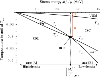
Figure 13: The plots of $T_{c\eta}$ evaluated by the Ginzburg-Landau analysis with typical parameter set $\Delta_{0}=25\,{\rm MeV}$ and $\mu=500\,{\rm MeV}$. When the coupling strength is increased, the critical DCP stress moves to higher value according to Eq. (45), while the ratio of $T_{c0}-T_{c3}:T_{c0}-T_{\rm DCP}=1:7$ would not be affected within the approximation we are working.

Let us now examine the case [B] with a relatively large strange quark mass. In this case, $\Delta_{1}$ first melts at $T_{c1}=T_{\rm ds}$ and after that, $\Delta_{2}$ disappears at $T_{c2}(>T_{c1})$; that is

$$\begin{array}[]{rcl}T_{c1}&=&\displaystyle T_{c0}\left[1-\log\left(\frac{\mu}{T_{c0}}\right)\frac{M_{s}^{2}}{6\mu^{2}}-\frac{35\zeta(3)\mu^{2}}{128\pi^{2}T_{c0}^{2}}\frac{M_{s}^{4}}{\mu^{4}}\right],\\[8.61108pt] T_{c2}&=&\displaystyle T_{c0}\left[1-\log\left(\frac{\mu}{T_{c0}}\right)\frac{13M_{s}^{2}}{24\mu^{2}}-\frac{7\zeta(3)\mu^{2}}{256\pi^{2}T_{c0}^{2}}\frac{M_{s}^{4}}{\mu^{4}}\right].\\[4.30554pt] \end{array}$$ (40)

In this case, the quark matter undergoes another hierarchical unlocking CFL $\to$ uSC $\to$ 2SC $\to$ UQM.

We have seen that the dSC phase is the second hottest pairing phase in the case [A], while the uSC phase takes over the dSC phase in the case [B]. One can see that the former (latter) situation will be realized at high (low) density. In fact, the case [A] includes the high density situation with the scale hierarchy

$$\frac{M_{s}^{2}}{2\mu}\ll M_{s}\ll(T_{c0},\Delta_{0})\ll\mu,$$ (41)

while the case [B] includes the low density regime with the scale hierarchy

$$(T_{c0},\Delta_{0}),\frac{M_{s}^{2}}{2\mu}\ll M_{s}\ll\mu.$$ (42)

Thus the case [B] contains an interesting regime with $\Delta_{0}\sim{M_{s}^{2}}/{2\mu}$ where the window for the gapless phases open at $T=0$. These two physically distinct regimes are separated by the doubly critical point (DCP) which was first discussed in the numerical analysis of the diquark NJL model Fukushima:2004zq . We can analytically derive the critical stress for the DCP point in our current framework as follows;

$$\left.\frac{M_{s}^{2}}{2\mu}\right|_{\rm DCP}(\mu,T_{c0})=\frac{16\pi^{2}}{21\zeta(3)}T_{c0}\left(\frac{T_{c0}}{\mu}\right)\log\left(\frac{\mu}{T_{c0}}\right).$$ (43)

Just at the density corresponding to this DCP point, we have a simultaneous melting of $\Delta_{1}$ and $\Delta_{2}$, and hence a direct transition CFL $\to$ 2SC takes place with increasing $T$ Fukushima:2004zq . We can express critical stress for the DCP in terms of the CFL gap $\Delta_{0}$ at $T=0$ and $M_{s}=0$ with the aid of the weak coupling universal relation

$$T_{c0}=2^{1/3}\frac{e^{\gamma}}{\pi}\Delta_{0}\cong 0.714\Delta_{0}.$$ (44)

Thus, the DCP point can be parameterized by the coupling strength $\Delta_{0}$ as

$$\left(\frac{M_{s}^{2}}{2\mu}\right)_{\rm DCP}=\Delta_{0}\frac{\Delta_{0}}{\mu}\left[1.07+3.19\log\left(\frac{\mu}{\Delta_{0}}\right)\right].$$ (45)

Also, the ratio of $T_{c0}$ to the CFL $\to$ 2SC transition temperature at the DCP point which we denote by $T_{\rm DCP}=T_{c1}=T_{c2}$ can be evaluated as

$$\frac{T_{\rm DCP}}{T_{c0}} = 1-\frac{8\pi^{2}}{9\zeta(3)}\left[\frac{T_{c0}}{\mu}\log\left(\frac{\mu}{T_{c0}}\right)\right]^{2}$$

$$= 1-\left(\frac{\Delta_{0}}{\mu}\right)^{2}\left[0.65+1.93\log\left(\frac{\mu}{\Delta_{0}}\right)\right]^{2}.$$

We can show the ratio

$$T_{c0}-T_{c3}^{\mbox{\scriptsize[2SC$\to$UQM]}}:T_{c0}-T_{\rm DCP}^{\mbox{\scriptsize[CFL$\to$2SC]}}=1:7$$ (47)

is universal being independent of the coupling choice $\Delta_{0}$.

	Regularization scheme	Theoretical parameters	Parameter regime of validity
Ginzburg-Landau theory	mass counter term	$T_{c0},M_{s},\mu$	$T\sim T_{c0}$, $\mu\gg M_{s},T_{c0}$	high density
Diquark NJL model	momentum cutoff	$\Lambda,G_{d},M_{s},\mu$	$\Lambda\mathrel{\mathchoice{\vbox{\offinterlineskip\halign{\hfil$\displaystyle#$\hfil\cr>\crcr\vskip 0.0pt\cr\sim\crcr}}}{\vbox{\offinterlineskip\halign{\hfil$\textstyle#$\hfil\cr>\crcr\vskip 0.0pt\cr\sim\crcr}}}{\vbox{\offinterlineskip\halign{\hfil$\scriptstyle#$\hfil\cr>\crcr\vskip 0.0pt\cr\sim\crcr}}}{\vbox{\offinterlineskip\halign{\hfil$\scriptscriptstyle#$\hfil\cr>\crcr\vskip 0.0pt\cr\sim\crcr}}}}\mu\mathrel{\mathchoice{\vbox{\offinterlineskip\halign{\hfil$\displaystyle#$\hfil\cr>\crcr\vskip 0.0pt\cr\sim\crcr}}}{\vbox{\offinterlineskip\halign{\hfil$\textstyle#$\hfil\cr>\crcr\vskip 0.0pt\cr\sim\crcr}}}{\vbox{\offinterlineskip\halign{\hfil$\scriptstyle#$\hfil\cr>\crcr\vskip 0.0pt\cr\sim\crcr}}}{\vbox{\offinterlineskip\halign{\hfil$\scriptscriptstyle#$\hfil\cr>\crcr\vskip 0.0pt\cr\sim\crcr}}}}\mu_{\chi\rm SB}$	moderate density

Table 2: The comparison of the Ginzburg-Landau theory and the diquark NJL model, i.e., the NJL model without the scalar $(q\bar{q})$-coupling Alford:2003fq ; Fukushima:2004zq ; Fukushima:2005fh . In the derivation of the Ginzburg-Landau potential, we adopt the regularization via the mass counter term (Thouless criterion), which insures that all the dimensionful mass scales vanish (correlation length diverges) at $T_{c0}$ when $M_{s}=0$. This regularization is model-independent in the sense that, after the prescription, the effective potential have neither $\Lambda$-dependence nor the explicit $G_{d}$-dependence. The Ginzburg-Landau approach is valid for the weak-coupling regime of QCD at high density ($\mu\gg M_{s},T_{c0}$), while the diquark NJL model is expected to describe the non-perturbavative regime of $(\Lambda\mathrel{\mathchoice{\vbox{\offinterlineskip\halign{\hfil$\displaystyle#$\hfil\cr>\crcr\vskip 0.0pt\cr\sim\crcr}}}{\vbox{\offinterlineskip\halign{\hfil$\textstyle#$\hfil\cr>\crcr\vskip 0.0pt\cr\sim\crcr}}}{\vbox{\offinterlineskip\halign{\hfil$\scriptstyle#$\hfil\cr>\crcr\vskip 0.0pt\cr\sim\crcr}}}{\vbox{\offinterlineskip\halign{\hfil$\scriptscriptstyle#$\hfil\cr>\crcr\vskip 0.0pt\cr\sim\crcr}}}}\mu\mathrel{\mathchoice{\vbox{\offinterlineskip\halign{\hfil$\displaystyle#$\hfil\cr>\crcr\vskip 0.0pt\cr\sim\crcr}}}{\vbox{\offinterlineskip\halign{\hfil$\textstyle#$\hfil\cr>\crcr\vskip 0.0pt\cr\sim\crcr}}}{\vbox{\offinterlineskip\halign{\hfil$\scriptstyle#$\hfil\cr>\crcr\vskip 0.0pt\cr\sim\crcr}}}{\vbox{\offinterlineskip\halign{\hfil$\scriptscriptstyle#$\hfil\cr>\crcr\vskip 0.0pt\cr\sim\crcr}}}}\mu_{\chi\rm SB})$, where $\mu_{\chi\rm SB}$ is the chemical potential for the chiral symmetry restoration.

FIG. 13 shows the phase diagram calculated with the Ginzburg-Landau potential for $\Delta_{0}=25\,{\rm MeV}$ and $\mu=500\,{\rm MeV}$, where the critical temperatures ($T_{c\eta}$) versus the stress energy $(M_{s}^{2}/\mu)$ is depicted by changing $M_{s}$ with $\mu$ fixed. The DCP is located at $(M_{s}^{2}/\mu)_{\rm DCP}=26.6\,{\rm MeV}\ll\mu=500\,{\rm MeV}$ and $T_{c}^{\rm DCP}/T_{c0}=0.90$. These values agree well with those obtained in the numerical analysis of the diquark NJL model where $(M_{s}^{2}/\mu)_{\rm DCP}\sim 30\,{\rm MeV}$ and $T_{c}^{\rm DCP}/T_{c0}\sim 0.85$ Fukushima:2004zq . If we increase the coupling to $\Delta_{0}=(40,100)\,{\rm MeV}$, then the DCP shifts to $(M_{s}^{2}/\mu)_{\rm DCP}=(58.5,248.4)\,{\rm MeV}$, and $T_{c}^{\rm DCP}/T_{c0}=(0.81,0.44)$ according to Eqs. (43) and (III.5). We can see that the agreement with the diquark NJL result Fukushima:2004zq becomes worse in the stronger coupling. This is because $M_{s}^{\rm DCP}$ shifts to higher value as $\Delta_{0}$ increases so that the Ginzburg-Landau approach becomes worse due to lack of the scale hierarchy $M_{s}\ll\mu$. In TABLE 2, we have summarized the parameter regime where the Ginzburg-Landau approach and the diquark NJL model are valid. It is worth stressing that according to the Ginzburg-Landau evaluation of the DCP given by Eq. (43), $(M_{s}^{2}/\mu)_{\rm DCP}$ is located around $\sim\Delta_{0}(\Delta_{0}/\mu)$, which is lower with a factor $\Delta_{c0}/\mu$ than $\Delta_{c0}$, i.e., the value corresponding to the interesting low density regime $M_{s}^{2}/\mu\sim\Delta_{0}$; the dSC phase is realized at higher density than the gCFL/CFL transition density.

In the following, we discuss where in the $(\mu,T)$-plane the DCP is located. We first discuss the possibility that it is in the moderate density regime using the diquark NJL model. Since the full thermodynamic potential should take the form like $\Omega(\mu,M_{s})=T_{c0}^{4}f(M_{s}/\mu,T_{c0}/\mu)$ and $T_{c0}/\mu$ is a slowly varying function of $\mu$, changing $M_{s}$ and changing $\mu$ are independent of each other in principle. If we fix $M_{s}$ to some value, we can obtain the phase diagram in the $(\mu,T)$-plane like FIG. 2 of Fukushima:2005fh by determining the phase by changing $(\mu,T)$; this is contrasted to FIG. 13 where $M_{s}$ is changed to control the density. In this case, we can find the unique DCP in $(\mu,T)$-plane, which we denote by $(\mu_{\rm DCP},T_{\rm DCP})\equiv(\mu,T)_{\rm DCP}$. We note that the DCP $(\mu,T)_{\rm DCP}$ shifts in $(\mu,T)$-plane if $M_{s}$ is changed. We have plotted the DCP $(\mu,T)_{\rm DCP}$ for several choice of $M_{s}$ in FIG. 14(a). Although we have used the same diquark NJL model as Fukushima:2005fh , we did not adopted the chemical potential shift approximation as is made there, but performed the exact treatment of $M_{s}$ since the condition $M_{s}\ll\mu$ does not hold well. As can be seen from the figure, as $M_{s}$ is increased, the DCP shifts to larger $\mu$ pushing away the dSC phase to higher density. We did not find the DCP for $M_{s}\mathrel{\mathchoice{\vbox{\offinterlineskip\halign{\hfil$\displaystyle#$\hfil\cr>\crcr\vskip 0.0pt\cr\sim\crcr}}}{\vbox{\offinterlineskip\halign{\hfil$\textstyle#$\hfil\cr>\crcr\vskip 0.0pt\cr\sim\crcr}}}{\vbox{\offinterlineskip\halign{\hfil$\scriptstyle#$\hfil\cr>\crcr\vskip 0.0pt\cr\sim\crcr}}}{\vbox{\offinterlineskip\halign{\hfil$\scriptscriptstyle#$\hfil\cr>\crcr\vskip 0.0pt\cr\sim\crcr}}}}187\,{\rm MeV}$, where we find only the uSC in the phase diagram. This may be a cutoff artifact because $\mu_{\rm DCP}$ increases with increasing $M_{s}$ and approaches $\Lambda=800\,{\rm MeV}$.

We have seen that the location of the DCP in the ($\mu,T$)-plane has one-to-one correspondence to the value of $M_{s}$. Conversely, if the DCP $(\mu,T)_{\rm DCP}$ is found for some fixed strange quark mass $M_{s}$, then this $M_{s}$ can be viewed as the doubly critical strange quark mass $M_{s}^{\rm DCP}$ for fixed chemical potential $\mu=\mu_{\rm DCP}$; this follows from the observation that the dSC (uSC) phase will be realized for $M_{s}<M_{s}^{\rm DCP}$ ($M_{s}>M_{s}^{\rm DCP}$) as can be expected from FIG. 13. In this sense, we have plotted the doubly critical strange quark mass $M_{s}^{\rm DCP}$ as a function of $\mu$ in FIG. 14(b). For $M_{s}$-region above (below) $M_{s}^{\rm DCP}(\mu)$ line, the uSC (dSC) phase would be realized. Just for comparison, we have also shown the weak coupling Ginzburg-Landau evaluation of the doubly critical strange quark mass, which can be obtained via putting $(\mu,T_{c0})$-relation into Eq. (43) (see solid line indicated by $M_{s}^{\rm DCP}(\mu,T_{c0})$). We can see the sizable deviation between these two lines, which is simply attributed to $M_{s}\hbox to10.00002pt{\hbox to0.0pt{\hbox to10.00002pt{\hss/\hss}\hss}\hbox{$\ll$}}\mu$. However, we stress that the qualitative behaviours are the same; if one goes higher density, the doubly critical strange quark mass shifts to larger value so that the dSC phase becomes robuster against the strange quark mass. In order to understand why the dSC does not appear in our model with the scalar coupling $G_{s}$ and $(q\bar{q})$-condensates, we have also plotted the dynamically determined strange quark mass in the $\chi$SB/UQM sector (see the solid line indicated by $M_{s}^{\chi\rm SB/UQM}$). The dynamical mass is evaluated on the $\mu$-$T_{c0}$ line in FIG. 14(a) so that it should be regarded as the lower limit of the dynamical strange quark mass in the superconducting phase. We can see that the line of $M_{s}^{\chi\rm SB/UQM}$ is well above the line for $M_{s}^{\rm DCP}(\mu)$ and the two lines never intersect for $\mu\mathrel{\mathchoice{\vbox{\offinterlineskip\halign{\hfil$\displaystyle#$\hfil\cr<\crcr\vskip 0.0pt\cr\sim\crcr}}}{\vbox{\offinterlineskip\halign{\hfil$\textstyle#$\hfil\cr<\crcr\vskip 0.0pt\cr\sim\crcr}}}{\vbox{\offinterlineskip\halign{\hfil$\scriptstyle#$\hfil\cr<\crcr\vskip 0.0pt\cr\sim\crcr}}}{\vbox{\offinterlineskip\halign{\hfil$\scriptscriptstyle#$\hfil\cr<\crcr\vskip 0.0pt\cr\sim\crcr}}}}\Lambda$, which provides one probable reason for the abscense of the dSC in the present NJL model with dynamical chiral condensates.

Let us finally discuss the possibility that the DCP is located in the weak coupling $(\mu,T)$-regime of QCD. In QCD, it should be unique because the strange quark mass $M_{s}$ is a decreasing function of $\mu$ approaching its current value $m_{s}\sim 100\,{\rm MeV}$ in the high density limit, while the doubly critical strange quark mass $M_{s}^{\rm DCP}$ is an increasing function of $\mu$. If we assume that the crossing (DCP) point $\mu=\mu^{*}$ at which $M_{s}^{\rm DCP}(\mu^{*})=M_{s}(\mu^{*})$ is located where $M_{s}^{\rm DCP}(\mu^{*})\ll\mu^{*}$, then we can estimate $\mu^{*}$ by the weak coupling Ginzburg-Landau result, Eq. (43). By using the universal relation, Eq. (44), and the weak coupling perturbative formula for gap, $\Delta_{0}(\mu)\sim\mu g^{-5}e^{-\frac{3\pi^{2}}{\sqrt{2}g}}$ Son:1998uk ; Schafer:1999jg as well, we have the formula $M_{s}^{\rm DCP}\sim\Delta_{0}(\mu)/\sqrt{\mathstrut g}$; this is actually a slowly increasing function of $\mu$ when $g$ is identified with the running coupling constant $\bar{g}(\mu)$ varying with $\mu$. According to the Schwinger-Dyson analysis of the gap Schafer:1999jg ; Rajagopal:2000rs ; Abuki:2001be , $\Delta_{0}(\mu)/\sqrt{\mathstrut\bar{g}(\mu)}$ reaches $\sim 100\,{\rm MeV}$ around $\mu\sim 10^{10}\,{\rm MeV}$; this indicates $\mu^{*}$ would be located at even higher chemical potential since $m_{s}\sim 100\,{\rm MeV}$ is the lower limit of the mass function $M_{s}(\mu)$. It should be also noted that our starting assumption $M_{s}^{\rm DCP}(\mu^{*})\ll\mu^{*}$ can be justified because the weak coupling condition $\Delta_{0}<\Delta_{0}(\mu^{*})/\sqrt{\mathstrut\bar{g}(\mu^{*})}\ll\mu^{*}$ is satisfied. We can conclude that the dSC phase is realized in the extremely high density regime of $\mu\mathrel{\mathchoice{\vbox{\offinterlineskip\halign{\hfil$\displaystyle#$\hfil\cr>\crcr\vskip 0.0pt\cr\sim\crcr}}}{\vbox{\offinterlineskip\halign{\hfil$\textstyle#$\hfil\cr>\crcr\vskip 0.0pt\cr\sim\crcr}}}{\vbox{\offinterlineskip\halign{\hfil$\scriptstyle#$\hfil\cr>\crcr\vskip 0.0pt\cr\sim\crcr}}}{\vbox{\offinterlineskip\halign{\hfil$\scriptscriptstyle#$\hfil\cr>\crcr\vskip 0.0pt\cr\sim\crcr}}}}\mu^{*}$ of QCD.

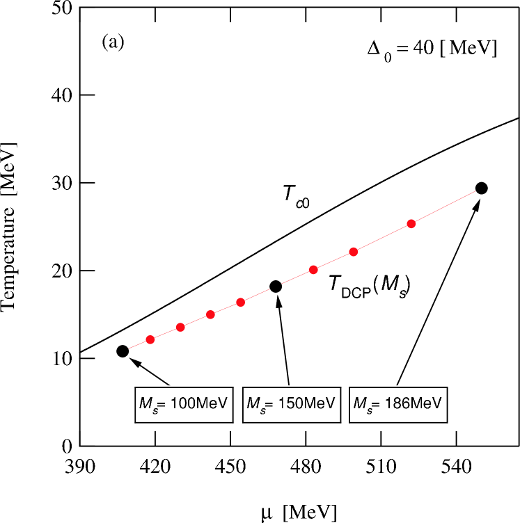
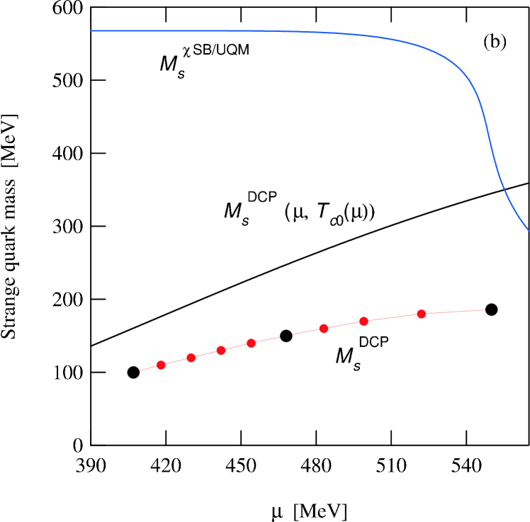
Figure 14: (a) The DCP point $(\mu,T)_{\rm DCP}$ for various value of $M_{s}$; from left to right, $M_{s}=100\,{\rm MeV},110\,{\rm MeV},\cdots,180\,{\rm MeV}$ and $M_{s}=186\,{\rm MeV}$. The quark-quark coupling $G_{d}$ is fixed so that $\Delta_{0}=40\,{\rm MeV}$ at $\mu=500\,{\rm MeV}$ as in Fukushima:2005fh . The solid line is $T_{c0}(\mu)$, i.e., the critical temperature for $M_{s}=0$ as a function of $\mu$. (b) The doubly critical strange quark mass $M_{s}^{\rm DCP}$ as a function of $\mu$. The solid line indicated by $M_{s}^{\rm DCP}(\mu,T_{c0}(\mu))$ represents the weak coupling Ginzburg-Landau evaluation of $M_{s}^{\rm DCP}$ by putting the numerical $\mu$-$T_{c0}$ relation depicted in (a) into Eq. (43). The solid line indicated by $M_{s}^{\chi\rm SB/UQM}$ is the dynamically determined strange quark mass in the $\chi$SB/UQM sector of our model with the scalar $(q\bar{q})$-coupling.

IV Summary and Outlook

In summary, we have investigated the QCD phase diagram with a special attention to the interplay between the chiral and diquark dynamics for a wide region of the diquark coupling strength. Our results for the two limiting cases, the intermediate and strong coupling, qualitatively agree with those obtained in the recent analyses Ruster:2005jc ; Blaschke:2005uj . Our central results can be summarized as follows. (i) As the diquark coupling is increased, the phase diagram gets gradually dominated by the fully gapped phases, while premature gapless phases get excluded out as is noted for $T=0$ in the previous work Abuki:2004zk . In particular, the phase diagram in the strong diquark coupling ($\Delta_{0}\mathrel{\mathchoice{\vbox{\offinterlineskip\halign{\hfil$\displaystyle#$\hfil\cr>\crcr\vskip 0.0pt\cr\sim\crcr}}}{\vbox{\offinterlineskip\halign{\hfil$\textstyle#$\hfil\cr>\crcr\vskip 0.0pt\cr\sim\crcr}}}{\vbox{\offinterlineskip\halign{\hfil$\scriptstyle#$\hfil\cr>\crcr\vskip 0.0pt\cr\sim\crcr}}}{\vbox{\offinterlineskip\halign{\hfil$\scriptscriptstyle#$\hfil\cr>\crcr\vskip 0.0pt\cr\sim\crcr}}}}160\,{\rm MeV}$) does not include gapless phases and hence the system is automatically free from the instability problem associated with imaginary Meissner masses. (ii) The second hottest pairing phase next to the 2SC phase depends on the quark density (and also on the diquark coupling strength). In particular, the dSC is not realized for all the parameter regions for which we have performed the calculation. This can be nicely understood by the Ginzburg-Landau analysis incorporating the quartic-order ($M_{s}^{4}$) effects to all the pair susceptibilities. In this analysis, we derived the analytical expression for the doubly critical point (DCP) Fukushima:2004zq at which the two second order critical lines intersect; one for the 2SC/dSC transition in the high density side and the other for the 2SC/uSC transition in the low density side. On the basis of this analysis, we conclude that the window for the dSC phase at high density $(T_{c0},\Delta_{0})\gg M_{s}$ tends to shrink as the density is lowered. (iii) We have demonstrated how and why non-trivial first order transition could be caused by the competition between the diquark and chiral condensations. (iv) We have studied how the 2SC/g2SC and the CFL/gCFL₈ transition is smeared by the thermal disturbance by regarding the electron density and color-neutral isospin density as the order parameters.

In this work, we ignored a Kobayashi-Maskawa-’t Hooft six quark interaction Hatsuda:1994pi ; Kunihiro:1987bb ; Bernard:1987sg , whose effect on the pairing is in part taken into account in Ruster:2005jc . This term, however, also brings a non-trivial interplay between the chiral and diquark dynamics through a mixed contraction like, $|\Delta_{3}|^{2}M_{s}$, for example; these terms indeed will be induced by the procedure of the mean field approximation. Also we have neglected a possible $K^{0}$ condensation in the CFL phase which may be relevant to the instability problem associated with the gapless phases Kryjevski:2004jw ; Buballa:2004sx . Examining this would require a further improvement of our understanding on how the meson spectroscopy on the CFL will be modified by the neutrality constraints He:2005mp . Extending current work so as to take these into account remains indeed an interesting future problem.

A number of papers have been devoted to the resolution of the imaginary Meissner masses in the gapless phases Unstable ; Fukushima:2005cm . These include; (i) exploring a possibility of the mixed phase Reddy:2004my along the line suggested earlier Neumann:2002jm ; Shovkovy:2003ce ; Bedaque:2003hi , (ii) the baryon current generation Huang:2005pv , (iii) examining the crystalline pairing phases Alford:2000ze taking the neutrality constraints into account Casalbuoni:2005zp ; Giannakis:2005sa , (iv) investigating a possible secondary gap formation Hong:2005jv , (v) the gluon condensation in the g2SC Gorbar:2005rx , and (vi) an inhomogeneous ($p$-wave) Kaon condensate Schafer:2005ym . Examining all these possibilities or searching for a more stable ground state as well as exploring a nature of the gluonic instability in the gapless phases is now one of central problems in QCD. Apart from this instability problem, we have shown that the chiral dynamics in the strange quark sector may simply wash out all the unstable regime of the gapless phases if the strength of the diquark coupling is large enough. It should be noted, however, that the $\mu$-window for g2SC phase still remains at $T=0$ in the phase diagram even for the diquark coupling $G_{d}/G_{s}=0.5$, i.e., the value extracted from one gluon exchange vertex. Determining the strength of the in-medium diquark coupling from the phenomenological studies including quark models applied to the exotic baryon spectroscopy as well as the lattice QCD simulation Nakamura:2004ur will be needed for a realistic description of the pairing dynamics at low density.

Appendix A Evaluation of Ginzburg-Landau coefficients

In this section, we present the detail for a derivation of Eq. (31). We work with the NJL model for a while, but the results will be found to be model-independent by a subtraction of the Thouless criterion: By this subtraction scheme, the model dependence is reduced only to the critical temperature $T_{c0}$.

We first expand Eq. (5) in terms of $\Delta$ at $T\sim T_{c0}$. Up to the quartic order in $\Delta$, we obtain

$${\mathcal{L}}_{\rm GL} = \Omega_{e}+\frac{4}{G_{d}}\sum_{\eta=1}^{3}\Delta_{\eta}^{2}$$

$$-T\sum_{n}\int\frac{d\mbox{\boldmath$p$}}{(2\pi)^{3}}\mbox{tr}{\rm Log}\left[{i\omega_{n}\mbox{\boldmath$1$}-{\mathcal{H}}^{0}_{36}}\right]$$

$$+{T}\sum_{m=1}^{4}\frac{1}{m}\sum_{n}\int\frac{d\mbox{\boldmath$p$}}{(2\pi)^{3}}\mbox{tr}\left[\frac{1}{i\omega_{n}\mbox{\boldmath$1$}-{\mathcal{H}}^{0}_{36}}{\mathcal{V}}_{36}\right]^{m},$$

where we have defined

$${\mathcal{H}}^{0}_{36}(\mbox{\boldmath$p$};\mbox{\boldmath$M$},\mbox{\boldmath$\mu$})={\mathcal{H}}_{36}|_{\mathstrut\mbox{\scriptsize{\boldmath$\Delta$}}\mathstrut\to 0},\,{\mathcal{V}}_{36}(\mbox{\boldmath$\Delta$})={\mathcal{H}}_{36}-{\mathcal{H}}^{0}_{36}.$$

We omitted the term for the mean-field potential of $M_{s}$ in Eq. (A) because we treat it as a constant and as if an external parameter near $T_{c}$. The zero-th order term involves the free quark contribution to the thermodynamic potential and the vacuum fluctuation which we shall simply subtract.

$$\begin{array}[]{c}\displaystyle-T\sum_{n}\int\frac{d\mbox{\boldmath$p$}}{(2\pi)^{3}}\mbox{tr}{\rm Log}\left[{i\omega_{n}\mbox{\boldmath$1$}-{\mathcal{H}}^{0}_{36}}\right]\\[4.30554pt] \displaystyle=\sum_{a,i}\Omega_{0}(M_{i},\mu_{ai},T)-2\sum_{a,i}\int\frac{d\mbox{\boldmath$p$}}{(2\pi)^{3}}E_{i},\\[4.30554pt] \end{array}$$ (49)

where $E_{i}=\sqrt{p^{2}+M_{i}^{2}}$ and

$$\Omega_{0}(M_{i},\mu_{ai},T) = -2T\int\frac{d\mbox{\boldmath$p$}}{(2\pi)^{3}}\log\left(1+e^{-(E_{i}-\mu_{ai})/T}\right)$$

$$-2T\int\frac{d\mbox{\boldmath$p$}}{(2\pi)^{3}}\log\left(1+e^{-(E_{i}+\mu_{ai})/T}\right).$$

Because ${\mathcal{H}}_{36}$ is block-diagonalized as ${\mathcal{H}}_{36}={\mathcal{H}}_{12}^{uds}\oplus\sum_{(\alpha,\beta)}^{(db,sg),(sr,ub),(ug,dr)}[({\mathcal{H}}^{\alpha\beta}_{4})\oplus(-{\mathcal{H}}^{\alpha\beta}_{4})]$, we can evaluate the quadratic and quartic terms for each sector separately as below.

$({\mathcal{H}}^{\alpha\beta}_{4})\oplus(-{\mathcal{H}}^{\alpha\beta}_{4})$ sector:

For the symmetry reason, we only have the term which is even order in $\Delta$. Thus we have to evaluate the quadratic and quartic terms in Eq. (A). The quadratic term can be regarded as the static susceptibility. For example, we define $\chi^{(db,sg)}$ for the $(\alpha,\beta)=(db,sg)$ sector by

$$\begin{array}[]{c}\displaystyle\frac{T}{2}\sum_{n}\int\!\!\!\frac{d\mbox{\boldmath$p$}}{(2\pi)^{3}}\mbox{tr}\left[\frac{1}{i\omega_{n}\mbox{\boldmath$1$}-{\mathcal{H}}^{\alpha\beta}_{4}}{\mathcal{V}}^{\alpha\beta}_{4}\right]^{2}+(i\omega_{n}\leftrightarrow-i\omega_{n})\\[17.22217pt] \displaystyle=-\Delta_{1}^{2}\chi^{(db,sg)}_{\mbox{\scriptsize 1-loop}}(0,\mbox{\boldmath$0$};\mu,T,\mu_{e},\mu_{3},\mu_{8},M_{s}).\\[4.30554pt] \end{array}$$ (50)

We can analytically evaluate $\chi_{\mbox{\scriptsize 1-loop}}^{(\alpha,\beta)}$ by expanding it in $\vec{t}=(M_{s}^{2}/\bar{\mu}_{\alpha\beta},\delta\mu_{\alpha\beta})$ with $\bar{\mu}_{\alpha\beta}\equiv(\mu_{\alpha}+\mu_{\beta})/2$ and $\delta\mu_{\alpha\beta}\equiv(\mu_{\alpha}-\mu_{\beta})/2$ being referred as the averaged and relative chemical potentials, respectively. Up to quartic order in $\vec{t}$, we obtain the following expression by performing all the Matsubara summations and the energy integrals except for the term suffering from the UV divergence,

$$\chi_{\mbox{\scriptsize 1-loop}}^{(db,sg)} = 2N[\bar{\mu}_{dbsg}]\biggl{(}1-\frac{M_{s}^{2}}{2\bar{\mu}_{dbsg}^{2}}\biggl{)}\int_{0}\!\!dE\frac{1}{E}{\tanh\left(\frac{E}{2T}\right)}$$ (51)

$$-N[\bar{\mu}_{dbsg}]\frac{7\zeta(3)M_{s}^{4}}{32\pi^{2}\bar{\mu}_{dbsg}^{2}T_{c}^{2}}$$

$$-N[\bar{\mu}_{dbsg}]\frac{7\zeta(3)\delta\mu_{dbsg}M_{s}^{2}}{4\pi^{2}\bar{\mu}_{dbsg}T_{c}^{2}}$$

$$-N[\bar{\mu}_{dbsg}]\frac{7\zeta(3)\delta\mu_{dbsg}^{2}}{2\pi^{2}T_{c}^{2}}.$$

To obtain this, we have ignored the contribution from quasi-antiquark poles. Also we have defined the density of state by $N[\mu]=\mu^{2}/2\pi^{2}$.

The term quartic in $\Delta_{1}$ can also be derived within the same approximation as done in the quadratic term:

$$N[\bar{\mu}_{dbsg}]\biggl{(}1-\frac{3M_{s}^{2}}{4\bar{\mu}_{dbsg}^{2}}\biggr{)}\frac{7\zeta(3)\Delta_{1}^{4}}{8\pi^{2}T_{c}^{2}}.$$ (52)

We note that order $\vec{t}$ correction corresponding to the second term in the above expression gives rise to an order $M_{s}^{4}$ correction to the critical temperature $T_{c\eta}$. However it can be shown that this correction to $T_{c\eta}$ is suppressed with a factor ${\mathcal{O}}(T_{c0}^{4}/\mu^{4})$ in comparison with that from the $t^{2}$ terms in the quadratic term in Eq. (51). Therefore we shall ignore the second term in Eq. (52) in the discussion below.

We have demonstrated the expansion in the case of $(db,sg)$ sector, but the Ginzburg-Landau coefficients in other two sectors, $(sr,ub)$ and $(ug,dr)$, can be derived in the completely same manner.

${\mathcal{H}}_{12}^{uds}$ sector:

Now we take care of the three-flavor mixed sector ${\mathcal{H}}_{12}^{uds}$. The terms quadratic in $\Delta$ can be shown to have the completely same form as that in the $({\mathcal{H}}_{4}^{\alpha\beta})\oplus(-{\mathcal{H}}_{4}^{\alpha\beta})$ sector. For instance, the term quadratic in $\Delta_{1}^{2}$ becomes

$$-\Delta_{1}^{2}\chi^{(dg,sb)}_{\mbox{\scriptsize 1-loop}},$$ (53)

where $\chi^{(dg,sb)}_{\mbox{\scriptsize 1-loop}}$ is defined by Eq. (51) with the replacement $(db,sg)\to(dg,sb)$. On the other hand, the quartic term coming from this sector turns out to be of the exotic form:

$$N[\bar{\mu}_{uds}]\frac{7\zeta(3)}{8\pi^{2}T_{c}^{2}}(\Delta_{1}^{2}+\Delta_{2}^{2}+\Delta_{3}^{2})^{2}$$

$$-N[\bar{\mu}_{uds}]\frac{M_{s}^{2}}{\mu_{uds}^{2}}\frac{21\zeta(3)}{32\pi^{2}T_{c}^{2}}(\Delta_{1}^{2}+\Delta_{2}^{2})(\Delta_{1}^{2}+\Delta_{2}^{2}+\Delta_{3}^{2}),$$

where we have defined $\bar{\mu}_{uds}\equiv(\mu_{ur}+\mu_{dg}+\mu_{sb})/3$. Also $M_{s}^{2}$ correction can be safely ignored in the analysis below for the same reason as given previously in the non-mixed two flavor sector.

Ginzburg-Landau potential:

We first investigate the ideal case of $M_{s}=\mu_{e,3,8}=0$. Combining all the results above and putting $M_{s}\to 0$ and $\mu_{e,3,8}\to 0$, we have

$${\mathcal{L}}_{\rm GL} = \sum_{\eta}\Delta_{\eta}^{2}\left[\frac{4}{G_{d}}-2\chi_{\mbox{\scriptsize 1-loop}}(0,\mbox{\boldmath$0$};\mu,T)\right]$$ (54)

$$+(\Delta_{1}^{4}+\Delta_{2}^{4}+\Delta_{3}^{4})N[\mu]\frac{7\zeta(3)}{8\pi^{2}T_{c}^{2}}$$

$$+(\Delta_{1}^{2}+\Delta_{2}^{2}+\Delta_{3}^{2})^{2}N[\mu]\frac{7\zeta(3)}{8\pi^{2}T_{c}^{2}}.$$

In this case all the susceptibilities $\chi_{\mbox{\scriptsize 1-loop}}^{(\alpha,\beta)}$ become of the same form and we denoted them by $\chi_{\mbox{\scriptsize 1-loop}}$. The quadratic term is divergent and needs a renormalization. We renormalize it with the use of the gap equation at $T=T_{c0}$ (The Thouless criterion for the critical temperature for three massless quark matter), which plays a role of the mass counter term in Bailin:1983bm :

$$\frac{4}{G_{d}}=2\chi_{\mbox{\scriptsize 1-loop}}(0,\mbox{\boldmath$0$},\mu,T_{c0}).$$ (55)

Subtracting this from the quadratic term, we obtain

$$\begin{array}[]{c}\displaystyle\Delta_{\eta}^{2}\left[\frac{4}{G_{d}}-2\chi_{\mbox{\scriptsize 1-loop}}(0,\mbox{\boldmath$0$};\mu,T)\right]\\[12.91663pt] \to\displaystyle 4\Delta_{1}^{2}N[\mu]\int_{0}\!dE\frac{1}{E}\left[\tanh\biggl{(}\frac{E}{2T_{c0}}\biggr{)}-\tanh\left(\frac{E}{2T}\right)\right]\\[12.91663pt] \cong\displaystyle 4\Delta_{1}^{2}N[\mu]\log\frac{T}{T_{c0}}\cong 4\Delta_{1}^{2}N[\mu]\frac{T-T_{c0}}{T_{c0}}.\\[4.30554pt] \end{array}$$ (56)

Using this, we obtain

$${\mathcal{L}}_{\rm GL} = (\Delta_{1}^{2}+\Delta_{2}^{2}+\Delta_{3}^{2})4N[{\mu}]\frac{T-T_{c0}}{T_{c0}}$$ (57)

$$+(\Delta_{1}^{4}+\Delta_{2}^{4}+\Delta_{3}^{4})\frac{7\zeta(3)N[\mu]}{8\pi^{2}T_{c0}^{2}}$$

$$+(\Delta_{1}^{2}+\Delta_{2}^{2}+\Delta_{3}^{2})^{2}\frac{7\zeta(3)N[\mu]}{8\pi^{2}T_{c0}^{2}}.$$

This is exactly of the same form as that obtained earlier in Iida:2000ha ; Iida:2002ev .

We now extend this result with the effects of strange quark mass and the charge neutrality constraints taken into account. Our task here is to calculate the splittings of the melting ($\Delta_{\eta}\to 0$) temperature $T_{c\eta}$ up to the quartic order in $M_{s}$. For this purpose, we need the expansion of the Ginzburg-Landau coefficients in terms of variables $t=(M_{s}^{2}/\mu,\mu_{e},\mu_{3},\mu_{8})$. In order to derive $T_{c\eta}$ up to the quartic order in $M_{s}$, we have to expand the coefficient of the quadratic term up to second order in $t$. Thus we start with the following Ginzburg-Landau potential.

$${\mathcal{L}}_{\rm GL} = \Omega_{e}(\mu_{e},T_{c})+\sum_{ai}\Omega_{0}(M_{i},\mu_{ai},T_{c})$$ (58)

$$+\Delta_{1}^{2}\left(\frac{4}{G_{d}}-\chi_{\mbox{\scriptsize 1-loop}}^{(dg,sb)}-\chi_{\mbox{\scriptsize 1-loop}}^{(db,sg)}\right)$$

$$+\Delta_{2}^{2}\left(\frac{4}{G_{d}}-\chi_{\mbox{\scriptsize 1-loop}}^{(sb,ur)}-\chi_{\mbox{\scriptsize 1-loop}}^{(sr,ub)}\right)$$

$$+\Delta_{3}^{2}\left(\frac{4}{G_{d}}-\chi_{\mbox{\scriptsize 1-loop}}^{(ur,dg)}-\chi_{\mbox{\scriptsize 1-loop}}^{(ug,dr)}\right)$$

$$+(\Delta_{1}^{4}+\Delta_{2}^{4}+\Delta_{3}^{4})\frac{7\zeta(3)N[\mu]}{8\pi^{2}T_{c0}^{2}}$$

$$+(\Delta_{1}^{2}+\Delta_{2}^{2}+\Delta_{3}^{2})^{2}\frac{7\zeta(3)N[\mu]}{8\pi^{2}T_{c0}^{2}}.$$

$4/G_{d}$ in the quadratic terms can again be replaced by $2\chi_{\mbox{\scriptsize 1-loop}}(0,\mbox{\boldmath$0$},\mu,T_{c0})$ by using the Thouless criterion in the symmetric matter Eq. (55). By doing this, the model dependence disappears and only its remnant is condensed into the parameter $T_{c0}$. After this replacement, we can expand the coefficients of $\Delta_{1}^{2}$, $\Delta_{2}^{2}$ and $\Delta_{3}^{2}$ in $t=(M_{s}^{2}/\mu,\mu_{e},\mu_{3},\mu_{8})$. For example, the $\Delta_{1}^{2}$ term can be expanded up to second order in $t$ as follows.

$$\begin{array}[]{rcl}\displaystyle\Delta_{1}^{2}\left(\frac{4}{G_{d}}-\chi_{\mbox{\scriptsize 1-loop}}^{(dg,sb)}-\chi_{\mbox{\scriptsize 1-loop}}^{(db,sg)}\right)&\to&\displaystyle N[\mu]\Delta_{1}^{2}\biggl{[}\frac{T-T_{c0}}{T_{c0}}\\[8.61108pt] &&\displaystyle+\left(\frac{2M_{s}^{2}}{\mu^{2}}-\frac{8\mu_{e}}{3\mu}+\frac{2\mu_{3}}{\mu}+\frac{4\mu_{8}}{3\mu}\right)\!\!\int_{0}\!dE\frac{1}{E}\tanh\left(\frac{E}{2T_{c0}}\right)\\[12.91663pt] &&\displaystyle-\biggl{(}\frac{3\mu_{3}+2\mu_{8}-4\mu_{e}}{6\mu}\biggr{)}^{2}\!\!\int_{0}\!dE\frac{1}{E}\tanh\left(\frac{E}{2T_{c0}}\right)\displaystyle+\frac{7\zeta(3)\mu^{2}}{16\pi^{2}T_{c0}^{2}}\biggl{\{}\frac{M_{s}^{4}}{\mu^{4}}+\left(\frac{\mu_{3}-2\mu_{8}}{\mu}\right)^{2}\biggr{\}}\biggr{]}.\\[8.61108pt] \end{array}$$ (59)

We have used the identity $N[\mu+\delta\mu]=N[\mu]+\mu\delta\mu/\pi^{2}+\delta\mu^{2}/2\pi^{2}$. Due to the asymmetries between cross-species which is caused by $M_{s}$ and $\{\mu_{e},\mu_{3},\mu_{8}\}$, we cannot completely eliminate the divergent quadratic term by the subtraction of the gap equation at $T_{c0}$ and we still have divergent corrections proportional to

$$\int_{0}^{\omega_{c}}\!dE\frac{1}{E}\tanh\left(\frac{E}{2T_{c0}}\right)=\log\left(\frac{2\omega_{c}e^{\gamma}}{\pi T_{c0}}\right),$$ (60)

with $\gamma$ being the Euler constant and $\omega_{c}$ is a UV cutoff for the quasi-quark energy. We note, however, that this divergence is originated simply in our constant gap parameter ansatz and can be made finite once the momentum dependence of the gap parameter is properly taken into account; it can be shown, in the same manner as adopted in Iida:2003cc , that we can replace the above divergent contribution by

$$\Delta_{\eta}^{2}\log\left(\frac{2\omega_{c}e^{\gamma}}{\pi T_{c0}}\right)\to\frac{1}{2}\Delta_{\eta}^{2}\log\left(\frac{\mu}{T_{c0}}\right)=\Delta_{\eta}^{2}\frac{3\sqrt{2}\pi^{2}}{4\bar{g}},$$ (61)

where $\Delta_{\eta}$ here should be regarded as the value of the gap energy at the Fermi-momentum $p=\mu$, and $\bar{g}$ is a running gauge coupling constant evaluated at energy scale $\mu$. In the following, we use the above formula instead of $\omega_{c}$-dependent expression. The $\Delta_{2}^{2}$ and $\Delta_{3}^{2}$ sectors can be evaluated in the similar way. After combining all the results, we have the full Ginzburg-Landau potential up to the quadratic order in $(M_{s}^{2}/\mu,\mu_{e},\mu_{3},\mu_{8})$:

$$\begin{array}[]{rcl}{\mathcal{L}}_{\rm GL}&=&\Omega_{e}(\mu_{e},T_{c0})+\sum_{ai}\Omega_{0}(M_{i},\mu_{ai},T_{c0})\\[8.61108pt] &&\displaystyle+(\Delta_{1}^{2}+\Delta_{2}^{2}+\Delta_{3}^{2})4N[\mu]\frac{T-T_{c0}}{T_{c0}}+\frac{7\zeta(3)N[\mu]}{8\pi^{2}T_{c0}^{2}}\left(\Delta_{1}^{4}+\Delta_{2}^{4}+\Delta_{3}^{4}\right)+\frac{7\zeta(3)N[\mu]}{8\pi^{2}T_{c0}^{2}}\left(\Delta_{1}^{2}+\Delta_{2}^{2}+\Delta_{3}^{2}\right)^{2}\\[8.61108pt] &&\displaystyle+N[\mu]\biggl{[}(\Delta_{1}^{2}+\Delta_{2}^{2})\frac{2M_{s}^{2}}{\mu^{2}}+\frac{4\mu_{e}}{3\mu}\left(-2\Delta_{1}^{2}+\Delta_{2}^{2}+\Delta_{3}^{2}\right)+\frac{2\mu_{3}}{\mu}(\Delta_{1}^{2}-\Delta_{2}^{2})+\frac{4\mu_{8}}{3\mu}(\Delta_{1}^{2}+\Delta_{2}^{2}-2\Delta_{3}^{2})\biggr{]}\frac{1}{2}\log\left(\frac{\mu}{T_{c0}}\right)\\[8.61108pt] &&\displaystyle-{N[\mu]}\biggl{[}\Delta_{1}^{2}\left(\frac{3\mu_{3}+2\mu_{8}-4\mu_{e}}{6\mu}\right)^{2}+\Delta_{2}^{2}\left(\frac{3\mu_{3}-2\mu_{e}-2\mu_{8}}{6\mu}\right)^{2}+4\Delta_{3}^{2}\left(\frac{\mu_{e}-2\mu_{8}}{6\mu}\right)^{2}\biggr{]}\frac{1}{2}\log\left(\frac{\mu}{T_{c0}}\right)\\[8.61108pt] &&\displaystyle+\frac{7\zeta(3)N[\mu]}{16\pi^{2}T_{c0}^{2}}\mu^{2}\biggl{[}\Delta_{1}^{2}\biggl{\{}\frac{M_{s}^{4}}{\mu^{4}}+\left(\frac{\mu_{3}-2\mu_{8}}{\mu}\right)^{2}\biggr{\}}+\Delta_{2}^{2}\biggl{\{}\left(\frac{\mu_{3}+2\mu_{8}}{\mu}\right)^{2}+\left(\frac{M_{s}^{2}}{\mu^{2}}-\frac{2\mu_{e}}{\mu}\right)^{2}\biggr{\}}+4\Delta_{3}^{2}\left(\frac{\mu_{e}^{2}-\mu_{3}^{2}}{\mu^{2}}\right)\biggr{]}.\\[8.61108pt] \end{array}$$ (62)

This is one of the central results from which the analytical expression for the splittings of the critical temperature ($T_{c0}\to T_{c\eta}$) can be derived (see Sec. III.5). We now impose the charge neutrality constraints by solving

$$\frac{\partial{\mathcal{L}}_{\rm GL}}{\partial\mu_{e}}=0,\quad\frac{\partial{\mathcal{L}}_{\rm GL}}{\partial\mu_{3}}=0,\quad\frac{\partial{\mathcal{L}}_{\rm GL}}{\partial\mu_{8}}=0,$$ (63)

in $\mu_{e},\mu_{3},\mu_{8}$. If $\Delta_{\eta}=0$, then the first condition above can be casted into the following familiar form of the balance equation under the weak coupling condition ($T\ll\mu$).

$$N_{c}\left(\frac{2}{3}\frac{p_{Fu}^{3}}{3\pi^{2}}-\frac{1}{3}\frac{p_{Fd}^{3}}{3\pi^{2}}-\frac{1}{3}\frac{p_{Fs}^{3}}{3\pi^{2}}\right)=\frac{\mu_{e}^{3}}{3\pi^{2}},$$ (64)

with

$$\begin{array}[]{rcl}p_{Fu}&=&\mu-\frac{2}{3}\mu_{e},\\[4.30554pt] p_{Fd}&=&\mu+\frac{1}{3}\mu_{e},\\[4.30554pt] p_{Fs}&=&\sqrt{(\mu+\frac{1}{3}\mu_{e})^{2}-M_{s}^{2}}.\\[4.30554pt] \end{array}$$ (65)

We can solve Eq. (64) order by order in $M_{s}$. Up to the quartic order in $M_{s}$, we obtain

$$\mu_{e}=\frac{M_{s}^{2}}{4\mu}-\frac{M_{s}^{4}}{48\mu^{3}}.$$ (66)

We here come back to Eq. (63), and solve these equations up to the quadratic order not only in $M_{s}^{2}/\mu$, but also in $\Delta_{\eta}$. We obtain

$$\mu_{e}=\frac{M_{s}^{2}}{4\mu}-\frac{M_{s}^{4}}{48\mu^{3}}-\frac{2\Delta_{1}^{2}-\Delta_{2}^{2}-\Delta_{3}^{2}}{6\mu}\log\left(\frac{\mu}{T_{c0}}\right),$$

$$\mu_{3}=\frac{\Delta_{1}^{2}-\Delta_{2}^{2}}{3\mu}\log\left(\frac{\mu}{T_{c0}}\right),$$

$$\mu_{8}=\frac{\Delta_{1}^{2}+\Delta_{2}^{2}-2\Delta_{3}^{2}}{6\mu}\log\left(\frac{\mu}{T_{c0}}\right).$$ (67)

Substituting these expression to the free potential $\Omega_{e}+\sum_{ai}\Omega_{0}$ and omitting terms which is independent of $\Delta_{\eta}$, we have the following $\Delta_{\eta}^{4}$ contribution

$$\begin{array}[]{c}\frac{8\Delta_{1}^{2}(\Delta_{2}^{2}+\Delta_{3}^{2})-8\Delta_{1}^{4}-5\Delta_{2}^{4}-5\Delta_{3}^{4}+2\Delta_{2}^{2}\Delta_{3}^{2}}{36\pi^{2}}\log\left(\frac{\mu}{T_{c0}}\right)^{2}.\\[4.30554pt] \end{array}$$

Also the feedback contribution to the quartic term comes from the quadratic $\Delta_{\eta}^{2}$ terms in Eq. (62). Substituting the chemical potentials to the quadratic terms in Eq. (62) leads to the following quartic terms.

$$\begin{array}[]{c}\frac{8\Delta_{1}^{4}+5\Delta_{2}^{2}+5\Delta_{3}^{4}-2\Delta_{2}^{2}\Delta_{3}^{2}-8\Delta_{1}^{2}(\Delta_{2}^{2}+\Delta_{3}^{2})}{18\pi^{2}}\log\left(\frac{\mu}{T_{c0}}\right)^{2}\\[8.61108pt] -(\Delta_{2}^{2}-\Delta_{3}^{2})(-2\Delta_{1}^{2}+\Delta_{2}^{2}+\Delta_{3}^{2})\frac{7\zeta(3)N[\mu]M_{s}^{2}}{48\pi^{2}\mu^{2}T_{c0}^{2}}\log\left(\frac{\mu}{T_{c0}}\right).\\[4.30554pt] \end{array}$$

These feedback terms bring about the $M_{s}^{2}$ ($M_{s}^{4}$) corrections to the critical temperatures $T_{c\eta}$, but these corrections are ${\mathcal{O}}(T_{c0}^{4}/\mu^{4})$ suppressed to those from $M_{s}^{2}$ ($M_{s}^{4}$) terms in the susceptibilities. Therefore, we can safely ignore these feedback contribution as long as $\mu\gg T_{c0}$. Substituting Eq. (67) into the quadratic and quartic terms of Eq. (62) and picking the parts which survives under $\mu\gg T_{c0}$ lead to our final result for the Ginzburg-Landau potential, i.e., Eq. (31). On the basis of this potential, we can argue how the CFL pairing gets dissolved when $T_{c0}$ is approached as is done in Sec. III.5.

In the present framework, we can also give the analytical formula for the following quantity,

$$\begin{array}[]{rcl}\displaystyle\frac{\Delta_{3}^{2}-\Delta_{2}^{2}}{\Delta_{1}^{2}-\Delta_{2}^{2}}\bigg{|}_{T\to T_{c0}}&\displaystyle=&\displaystyle 2+\frac{21\zeta(3)}{16\pi^{2}}\frac{M_{s}^{2}}{T_{c0}^{2}\log(\mu/T_{c0})}+\cdots.\\[8.61108pt] \end{array}$$ (68)

We have derived this expression starting with the Ginzburg-Landau potential. Conversely, if the $M_{s}$-dependence of this quantity is known, it gives some information about the $M_{s}$-dependent terms in the Ginzburg-Landau potential. In Fukushima:2004zq , this quantity is expanded as $\frac{\Delta_{3}^{2}-\Delta_{2}^{2}}{\Delta_{1}^{2}-\Delta_{2}^{2}}\big{|}_{T\to T_{c0}}=a+b\big{(}\frac{M_{s}}{\mu}\big{)}^{2}+c\big{(}\frac{M_{s}}{\mu}\big{)}^{4}+\cdots$, and the coefficients, $a,b$ and $c$, are extracted from the numerical result of the diquark NJL model; $a=2.52$, $b=36.2$ and $c=1.02\times 10^{3}$ are obtained with a parameter choice $(\mu,\Delta_{0})=(500,\,25)\,{\rm MeV}$. We find here, however, that Eq. (68) does not take a form of a simple expansion in $\big{(}\frac{M_{s}}{\mu}\big{)}^{2}$ but rather seems to be an expansion in $\frac{M_{s}^{2}}{T_{c0}^{2}\log(\mu/T_{c0})}=\frac{\mu^{2}}{T_{c0}^{2}\log(\mu/T_{c0})}\big{(}\frac{M_{s}}{\mu}\big{)}^{2}$. This may explain unusually large numerical values of $b$ and $c$.

Appendix B Off-diagonal color densities

Here, we show that the off-diagonal color densities automatically vanish for the standard ansatz with the diquark condensate, i.e., Eq. (14). To prove this, we include the chemical potentials not only for the diagonal but also for off-diagonal color charges as given in Eq. (3). The Nambu-Gor’kov Hamiltonian density in this case takes the following form after spin-degeneracy removing,

$${\scriptsize{\mathcal{H}}_{36}\!=\!\left(\begin{array}[]{ccccccccc}H_{ur}&D_{3}&D_{2}&&M_{12}^{\dagger}&&M_{45}^{\dagger}&&\\ D_{3}&H_{dg}&D_{1}&M_{12}&&&&&M_{67}^{\dagger}\\ D_{2}&D_{1}&H_{sb}&&&M_{45}&&M_{67}&\\ &M_{12}^{\dagger}&&H_{dr}&-D_{3}&&&&M_{45}^{\dagger}\\ M_{12}&&&-D_{3}&H_{ug}&&M_{67}^{\dagger}&&\\ &&M_{45}^{\dagger}&&&H_{sr}&-D_{2}&M_{12}^{\dagger}&\\ M_{45}&&&&M_{67}&-D_{2}&H_{ub}&&\\ &&M_{67}^{\dagger}&&&M_{12}&&H_{sg}&-D_{1}\\ &M_{67}&&M_{45}&&&&-D_{1}&H_{db}\\ \end{array}\right)},$$ (69)

where all the matrix elements are $4\times 4$ matrices defined by

$$\begin{array}[]{rcl}H_{ia}\!&=&\!\left(\begin{array}[]{cccc}\!M_{i}\!-\!\mu_{ai}\!&p&&\\ p&\!-M_{i}\!-\!\mu_{ai}\!&&\\ &&\!M_{i}\!+\!\mu_{ai}\!&-p\\ &&-p&\!-M_{i}\!+\!\mu_{ai}\!\\ \end{array}\right),\\[8.61108pt] D_{\eta}\!&=&\!\left(\begin{array}[]{cccc}&&&-i\Delta_{\eta}\\ &&-i\Delta_{\eta}&\\ &i\Delta_{\eta}&&\\ i\Delta_{\eta}&&&\\ \end{array}\right),\\[8.61108pt] M_{\alpha\beta}\!&=&\!\left(\begin{array}[]{cccc}\!\!\mu_{\alpha}\!+\!i\mu_{\beta}\!\!&&&\\ &\!\!\mu_{\alpha}\!+\!i\mu_{\beta}\!\!&&\\ &&\!\!-\mu_{\alpha}\!+\!i\mu_{\beta}\!\!&\\ &&&\!\!-\mu_{\alpha}\!+\!i\mu_{\beta}\!\!\\ \end{array}\right),\\[8.61108pt] \end{array}$$ (70)

respectively. We define ${\mathcal{H}}_{36}^{0}$ by putting $\mu_{1}=\mu_{2}=\mu_{4}=\mu_{5}=\mu_{6}=\mu_{7}=0$ in Eq. (69).

$${\scriptsize{\mathcal{H}}_{36}^{0}\!=\!\left(\begin{array}[]{ccccccccc}H_{ur}&D_{3}&D_{2}&&&&&&\\ D_{3}&H_{dg}&D_{1}&&&&&&\\ D_{2}&D_{1}&H_{sb}&&&&&&\\ &&&H_{dr}&-D_{3}&&&&\\ &&&-D_{3}&H_{ug}&&&&\\ &&&&&H_{sr}&-D_{2}&&\\ &&&&&-D_{2}&H_{ub}&&\\ &&&&&&&H_{sg}&-D_{1}\\ &&&&&&&-D_{1}&H_{db}\\ \end{array}\right)},$$ (71)

This Hamiltonian density ${\mathcal{H}}_{36}^{0}$ can be further reduced to the block-diagonalized form as given in the text after some unitary transformation which makes the Nambu-Gor’kov doubling explicit in the $(ug,dr)$, $(db,sg)$ and $(sr,ub)$ sectors. However this is not necessary in the following argument, so we proceed further with Eq. (71).

We now define the off-diagonal color charge matrices in the Nambu-Gor’kov bases as

$$\mbox{\boldmath$Q$}_{\alpha}=-\frac{\partial{\mathcal{H}}_{36}}{\partial\mu_{\alpha}},$$ (72)

with $\alpha=1,2,4,5,6,7$ in addition to the diagonal charges

$$\mbox{\boldmath$Q$}_{e,3,8}=-\frac{\partial{\mathcal{H}}_{36}}{\partial\mu_{e,3,8}}.$$ (73)

What we have to show is that the off-diagonal color densities automatically vanish on the ground state determined by ${\mathcal{H}}^{0}_{36}$. To see this, we first define the complete sets by the following eigen-value equation:

$${\mathcal{H}}_{36}^{0}|p,\alpha,\sigma\rangle^{0}=\sigma\varepsilon_{\alpha}^{0}(p)|p,\alpha,\sigma\rangle^{0}.$$ (74)

We have 36 eigenvalues which we distinguish by $\alpha=1,2,\cdots 18$ and the Nambu-Gor’kov spin $\sigma=\pm$. The off-diagonal color densities can be written in the form as in Sec. II.2,

$$\begin{array}[]{rcl}\rho_{\alpha}\!\!&=&\!\!-\frac{1}{2}\sum_{\alpha=1}^{18}\int\!\!\!\frac{d\mathstrut\mbox{\scriptsize{\boldmath$p$}}\mathstrut}{(2\pi)^{3}}\tanh\left(\frac{\varepsilon_{\alpha}^{0}}{2T}\right){}^{0}\langle p,\alpha,+|\mbox{\boldmath$Q$}_{\alpha}|p,\alpha,+\rangle^{0}\\[8.61108pt] \!\!&&\!\!+\frac{1}{2}\sum_{\alpha=1}^{18}\int\!\!\!\frac{d\mathstrut\mbox{\scriptsize{\boldmath$p$}}\mathstrut}{(2\pi)^{3}}\tanh\left(\frac{\varepsilon_{\alpha}^{0}}{2T}\right){}^{0}\langle p,\alpha,-|\mbox{\boldmath$Q$}_{\alpha}|p,\alpha,-\rangle^{0}.\end{array}$$ (75)

The ${\tilde{Q}}$ charge matrix in the Nambu-Gor’kov bases

$$\mbox{\boldmath${\tilde{Q}}$}=-\mbox{\boldmath$Q$}_{e}-\mbox{\boldmath$Q$}_{3}-\frac{1}{2}\mbox{\boldmath$Q$}_{8}$$ (76)

commutes with the Hamiltonian density ${\mathcal{H}}_{36}^{0}$, i.e., $[{\mathcal{H}}_{36}^{0},\mbox{\boldmath${\tilde{Q}}$}]=0$, so that the quasi-particle states $|p,\alpha,\pm\rangle^{0}$ can be chosen to be the eigenstates of ${\tilde{Q}}$. Also we note

$$\begin{array}[]{rcl}\mbox{\boldmath$Q$}_{1}&=&-i[\mbox{\boldmath${\tilde{Q}}$},\,\mbox{\boldmath$Q$}_{2}],\\[8.61108pt] \mbox{\boldmath$Q$}_{2}&=&+i[\mbox{\boldmath${\tilde{Q}}$},\,\mbox{\boldmath$Q$}_{1}],\\[8.61108pt] \mbox{\boldmath$Q$}_{4}&=&-i[\mbox{\boldmath${\tilde{Q}}$},\,\mbox{\boldmath$Q$}_{5}],\\[8.61108pt] \mbox{\boldmath$Q$}_{5}&=&+i[\mbox{\boldmath${\tilde{Q}}$},\,\mbox{\boldmath$Q$}_{4}].\\[8.61108pt] \end{array}$$ (77)

From these commutation relations, we can immediately conclude

$$\rho_{1}=\rho_{2}=\rho_{4}=\rho_{5}=0,$$ (78)

because

$$\begin{array}[]{c}{}^{0}\langle p,\alpha,\sigma|\mbox{\boldmath$Q$}_{1}|p,\alpha,\sigma\rangle^{0}=i\,{}^{0}\langle p,\alpha,\sigma|[\mbox{\boldmath$Q$}_{2},\,\mbox{\boldmath${\tilde{Q}}$}]|p,\alpha,\sigma\rangle^{0}=0\\[8.61108pt] \end{array}$$ (79)

This conclusion follows from ${\tilde{Q}}$ is diagonal in the quasi-particle bases,

$${}^{0}\langle p,\alpha,\sigma|\mbox{\boldmath${\tilde{Q}}$}|p,\beta,\sigma^{\prime}\rangle^{0}=q_{\alpha}^{\sigma}\delta_{\alpha\beta}\delta_{\sigma\sigma^{\prime}},$$ (80)

where $q_{\alpha}^{\sigma}$ takes the values $(-1,0,+1)$.

In contrast, the disappearances of $\rho_{6}$ and $\rho_{7}$ cannot be proven in the same manner because of the commutation relations:

$$i[\mbox{\boldmath${\tilde{Q}}$},\,\mbox{\boldmath$Q$}_{6}]=0,\quad i[\mbox{\boldmath${\tilde{Q}}$},\,\mbox{\boldmath$Q$}_{7}]=0.$$ (81)

Thus we try to give a more direct proof here. We first re-write Eq. (75) as

$$\begin{array}[]{rcl}\rho_{\alpha}\!\!&=&\displaystyle\!\!-\frac{1}{2}\sum_{\sigma,\alpha}\int\!\!\!\frac{d\mbox{\boldmath$p$}}{(2\pi)^{3}}{}^{0}\langle p,\alpha,\sigma|\tanh\left(\frac{{\mathcal{H}}_{36}^{0}}{2T}\right)\mbox{\boldmath$Q$}_{\alpha}|p,\alpha,\sigma\rangle^{0}\\[8.61108pt] \!\!&=&\displaystyle\!\!-\frac{1}{2}\sum_{\sigma,\alpha}\int\!\!\!\frac{d\mbox{\boldmath$p$}}{(2\pi)^{3}}{\mbox{tr}}\left[\tanh\left(\frac{{\mathcal{H}}_{36}^{0}}{2T}\right)\mbox{\boldmath$Q$}_{\alpha}\right].\\[4.30554pt] \end{array}$$ (82)

Since the trace does not depend on the base, we can evaluate the trace with the natural base instead of the quasi-particle eigen-spinors. Thus what we have to show here turns out to be the proof of

$${\mbox{tr}}\left[{\mathcal{H}}_{36}^{0}\mbox{\boldmath$Q$}_{6,7}\right]=0,\,{\mbox{tr}}\left[{\mathcal{H}}_{36}^{0}{\mathcal{H}}_{36}^{0}{\mathcal{H}}_{36}^{0}\mbox{\boldmath$Q$}_{6,7}\right]=0,\,\cdots.$$ (83)

If this infinite series of conditions can be shown to be true, then we can conclude

$$\rho_{6}=\rho_{7}=0.$$ (84)

Using the explicit form of the matrices ${\mathcal{H}}_{36}^{0}$ and $\mbox{\boldmath${\tilde{Q}}$}_{6,7}$, we have explicitly checked using the Mathematica, that the equation

$${\mbox{tr}}\left[({\mathcal{H}}_{36}^{0})^{2n-1}\mbox{\boldmath$Q$}_{6,7}\right]=0$$ (85)

indeed holds for $n=1,2,\cdots,18$. We have not confirmed Eq. (85) for $n>18$, but the confirmation up to $n\leq 18$ is adequate for the reason we shall give in the following.

First, we write the Hamiltonian density

$$\begin{array}[]{c}{\mathcal{H}}_{36}^{0}=\displaystyle\sum_{\sigma,\alpha}\sigma\varepsilon_{\alpha}(p)P_{\sigma\alpha}=\displaystyle\sum_{\alpha=1}^{18}(P_{\alpha}-P_{-\alpha})\varepsilon_{\alpha}(p),\end{array}$$ (86)

where $P_{\sigma\alpha}$ is the projection operator $|p,\alpha,\sigma\rangle^{0}{{}^{0}}\langle p,\alpha,\sigma|$ in the natural base; this operator projects vectors out to the eigenspace in which ${\mathcal{H}}_{36}^{0}=\sigma\varepsilon_{\alpha}(p)$ holds. Using this decomposition, we can re-write the 18 conditions as

$$\begin{array}[]{rrcl}1:&0&=&\sum_{\alpha=1}^{18}\varepsilon_{\alpha}\mbox{tr}\left[(P_{\alpha}-P_{-\alpha})\mbox{\boldmath$Q$}_{6,7}\right],\\[8.61108pt] 2:&0&=&\sum_{\alpha=1}^{18}\varepsilon_{\alpha}^{3}\mbox{tr}\left[(P_{\alpha}-P_{-\alpha})\mbox{\boldmath$Q$}_{6,7}\right],\\[8.61108pt] &\vdots&\\[8.61108pt] 18:&0&=&\sum_{\alpha=1}^{18}\varepsilon_{\alpha}^{35}\mbox{tr}\left[(P_{\alpha}-P_{-\alpha})\mbox{\boldmath$Q$}_{6,7}\right].\\[8.61108pt] \end{array}$$ (87)

If all the eighteen roots $\{\varepsilon_{\alpha}\}$ with $\alpha=1,2,\cdots,18$ take different values, then the above eighteen conditions simply mean

$$\mbox{tr}\left[(P_{\alpha}-P_{-\alpha})\mbox{\boldmath$Q$}_{6,7}\right]=0,$$ (88)

for $\alpha=1,2,\cdots,18$. Therefore for the arbitrary integer $n$, $\mbox{tr}[({\mathcal{H}}_{32}^{0})^{2n-1}\mbox{\boldmath$Q$}_{6,7}]=0$ should hold. In the case that the degeneracy is present as $\varepsilon_{1}=\varepsilon_{2}=\varepsilon_{3}$, for example, we can prove the following equation in the totally same manner as in the above argument,

$$\sum_{\alpha=1,2,3}\mbox{tr}\left[(P_{\alpha}-P_{-\alpha})\mbox{\boldmath$Q$}_{6,7}\right]=0,$$ (89)

and again reach the same conclusion $\mbox{tr}[({\mathcal{H}}_{32}^{0})^{2n-1}\mbox{\boldmath$Q$}_{6,7}]=0$. Thus, we have proven that the following condition indeed holds for $\alpha=6$ and $7$,

$$\begin{array}[]{c}\displaystyle{\mbox{tr}}\left[\tanh\left(\frac{{\mathcal{H}}_{36}^{0}}{2T}\right)\mbox{\boldmath$Q$}_{\alpha}\right]=0.\\[4.30554pt] \end{array}$$ (90)

Consequently, we reached the fact that all the off-diagonal color densities automatically vanish under the assumption of the diquark condensate given in Eq. (14).

References

- (1)
- (2) D. Bailin and A. Love, Phys. Rept. 107 (1984) 325.
- (3) M. Iwasaki and T. Iwado, Phys. Lett. B 350 (1995) 163.
- (4) For reviews, see K. Rajagopal and F. Wilczek, arXiv:hep-ph/0011333; M. G. Alford, Ann. Rev. Nucl. Part. Sci. 51, 131 (2001) [arXiv:hep-ph/0102047]; G. Nardulli, Riv. Nuovo Cim. 25N3, 1 (2002) [arXiv:hep-ph/0202037]; S. Reddy, Acta Phys. Polon. B 33, 4101 (2002) [arXiv:nucl-th/0211045]; T. Schäfer, arXiv:hep-ph/0304281; M. Alford, Prog. Theor. Phys. Suppl. 153, 1 (2004) [arXiv:nucl-th/0312007].
- (5) M. G. Alford, K. Rajagopal and F. Wilczek, Nucl. Phys. B 537, 443 (1999) [arXiv:hep-ph/9804403].
- (6) M. G. Alford, J. Berges and K. Rajagopal, Nucl. Phys. B 558 (1999) 219 [arXiv:hep-ph/9903502].
- (7) T. Schäfer and F. Wilczek, Phys. Rev. D 60, 074014 (1999) [arXiv:hep-ph/9903503].
- (8) H. Abuki, Prog. Theor. Phys. 110, 937 (2003) [arXiv:hep-ph/0306074].
- (9) K. Iida and G. Baym, Phys. Rev. D 63, 074018 (2001) [Erratum-ibid. D 66, 059903 (2002)] [arXiv:hep-ph/0011229].
- (10) K. Rajagopal and F. Wilczek, Phys. Rev. Lett. 86, 3492 (2001) [arXiv:hep-ph/0012039].
- (11) M. Alford and K. Rajagopal, JHEP 0206, 031 (2002) [arXiv:hep-ph/0204001].
- (12) M. Alford, C. Kouvaris and K. Rajagopal, Phys. Rev. Lett. 92, 222001 (2004) [arXiv:hep-ph/0311286]; Phys. Rev. D 71, 054009 (2005) [arXiv:hep-ph/0406137].
- (13) M. Alford, P. Jotwani, C. Kouvaris, J. Kundu and K. Rajagopal, Phys. Rev. D 71, 114011 (2005) [arXiv:astro-ph/0411560].
- (14) M. Huang and I. A. Shovkovy, Phys. Rev. D 70, 094030 (2004) [arXiv:hep-ph/0408268]; Phys. Rev. D 70 (2004) 051501 [arXiv:hep-ph/0407049]; R. Casalbuoni, R. Gatto, M. Mannarelli, G. Nardulli and M. Ruggieri, Phys. Lett. B 605 (2005) 362 [Erratum-ibid. B 615 (2005) 297] [arXiv:hep-ph/0410401]; I. Giannakis and H. C. Ren, Phys. Lett. B 611 (2005) 137 [arXiv:hep-ph/0412015]; Nucl. Phys. B 723, 255 (2005) [arXiv:hep-th/0504053]; for a general argument on the emergence of the imaginary Meissner mass in a gapless phase, see, M. Alford and Q. h. Wang, J. Phys. G 31 (2005) 719 [arXiv:hep-ph/0501078].
- (15) K. Fukushima, Phys. Rev. D 72, 074002 (2005) [arXiv:hep-ph/0506080].
- (16) S. Reddy and G. Rupak, Phys. Rev. C 71 (2005) 025201 [arXiv:nucl-th/0405054].
- (17) M. Huang, arXiv:hep-ph/0504235.
- (18) R. Casalbuoni, R. Gatto, N. Ippolito, G. Nardulli and M. Ruggieri, Phys. Lett. B 627, 89 (2005) [arXiv:hep-ph/0507247].
- (19) I. Giannakis, D. f. Hou and H. C. Ren, Phys. Lett. B 631, 16 (2005) [arXiv:hep-ph/0507306].
- (20) D. K. Hong, arXiv:hep-ph/0506097; M. Alford and Q. h. Wang, arXiv:hep-ph/0507269.
- (21) E. V. Gorbar, M. Hashimoto and V. A. Miransky, arXiv:hep-ph/0507303; arXiv:hep-ph/0509334.
- (22) T. Schäfer, arXiv:hep-ph/0508190.
- (23) K. Iida, T. Matsuura, M. Tachibana and T. Hatsuda, Phys. Rev. Lett. 93 (2004) 132001 [arXiv:hep-ph/0312363]; Phys. Rev. D 71, 054003 (2005) [arXiv:hep-ph/0411356].
- (24) K. Fukushima, C. Kouvaris and K. Rajagopal, Phys. Rev. D 71, 034002 (2005) [arXiv:hep-ph/0408322].
- (25) H. Abuki, M. Kitazawa and T. Kunihiro, Phys. Lett. B 615, 102 (2005) [arXiv:hep-ph/0412382].
- (26) S. B. Rüster, I. A. Shovkovy and D. H. Rischke, Nucl. Phys. A 743, 127 (2004) [arXiv:hep-ph/0405170].
- (27) G. Sarma, Phys. Chem. Solid 24, 1029 (1963).
- (28) H. Abuki, Master thesis submitted to Kyoto University (2000).
- (29) M. Kitazawa, T. Koide, T. Kunihiro and Y. Nemoto, Prog. Theor. Phys. 108 (2002) 929 [arXiv:hep-ph/0207255].
- (30) S. B. Rus̈ter, V. Werth, M. Buballa, I. A. Shovkovy and D. H. Rischke, Phys. Rev. D 72 (2005) 034004 [arXiv:hep-ph/0503184].
- (31) D. Blaschke, S. Fredriksson, H. Grigorian, A. M. Oztas and F. Sandin, Phys. Rev. D 72, 065020 (2005) [arXiv:hep-ph/0503194].
- (32) S. B. Rüster, V. Werth, M. Buballa, I. A. Shovkovy and D. H. Rischke, arXiv:hep-ph/0509073.
- (33) M. Buballa and I. A. Shovkovy, Phys. Rev. D 72, 097501 (2005) [arXiv:hep-ph/0508197].
- (34) A. W. Steiner, S. Reddy and M. Prakash, Phys. Rev. D 66 (2002) 094007 [arXiv:hep-ph/0205201].
- (35) M. Buballa and M. Oertel, Nucl. Phys. A 703 (2002) 770 [arXiv:hep-ph/0109095].
- (36) M. Buballa, Phys. Rept. 407 (2005) 205 [arXiv:hep-ph/0402234].
- (37) According to private communication with S. Fredrik, Ref. Blaschke:2005uj also uses the similar method to evaluate the derivatives of the thermodynamic potential.
- (38) A. Ali Khan et al. [CP-PACS Collaboration], Phys. Rev. D 65 (2002) 054505 [Erratum-ibid. D 67 (2003) 059901] [arXiv:hep-lat/0105015].
- (39) T. Hatsuda and T. Kunihiro, Phys. Rept. 247 (1994) 221 [arXiv:hep-ph/9401310].
- (40) D. B. Kaplan and A. E. Nelson, Phys. Lett. B 175 (1986) 57.
- (41) P. F. Bedaque and T. Schäfer, Nucl. Phys. A 697 (2002) 802 [arXiv:hep-ph/0105150]; D. B. Kaplan and S. Reddy, Phys. Rev. D 65, 054042 (2002) [arXiv:hep-ph/0107265].
- (42) I. Shovkovy and M. Huang, Phys. Lett. B 564, 205 (2003) [arXiv:hep-ph/0302142]; M. Huang and I. Shovkovy, Nucl. Phys. A 729, 835 (2003) [arXiv:hep-ph/0307273].
- (43) F. Sandin and A. M. Oztas, arXiv:hep-ph/0512087.
- (44) Y. Nishida and H. Abuki, Phys. Rev. D 72, 096004 (2005) [arXiv:hep-ph/0504083].
- (45) K. Fukushima, arXiv:hep-ph/0510299.
- (46) D. T. Son, Phys. Rev. D 59, 094019 (1999) [arXiv:hep-ph/9812287].
- (47) T. Schäfer and F. Wilczek, Phys. Rev. D 60, 114033 (1999) [arXiv:hep-ph/9906512]; W. E. Brown, J. T. Liu and H. c. Ren, Phys. Rev. D 61, 114012 (2000) [arXiv:hep-ph/9908248]; Phys. Rev. D 62, 054016 (2000) [arXiv:hep-ph/9912409].
- (48) K. Rajagopal and E. Shuster, Phys. Rev. D 62 (2000) 085007 [arXiv:hep-ph/0004074].
- (49) H. Abuki, T. Hatsuda and K. Itakura, Phys. Rev. D 65, 074014 (2002) [arXiv:hep-ph/0109013].
- (50) T. Kunihiro and T. Hatsuda, Phys. Lett. B 206, 385 (1988) [Erratum-ibid. 210, 278 (1988)];
- (51) V. Bernard, R. L. Jaffe and U. G. Meissner, Nucl. Phys. B 308, 753 (1988).
- (52) A. Kryjevski and T. Schäfer, Phys. Lett. B 606, 52 (2005) [arXiv:hep-ph/0407329]; A. Kryjevski and D. Yamada, Phys. Rev. D 71, 014011 (2005) [arXiv:hep-ph/0407350].
- (53) M. Buballa, Phys. Lett. B 609, 57 (2005) [arXiv:hep-ph/0410397]; M. M. Forbes, arXiv:hep-ph/0411001.
- (54) L. y. He, M. Jin and P. f. Zhuang, arXiv:hep-ph/0504148; D. Ebert, K. G. Klimenko and V. L. Yudichev, Phys. Rev. D 72, 056007 (2005) [arXiv:hep-ph/0504218].
- (55) F. Neumann, M. Buballa and M. Oertel, Nucl. Phys. A 714 (2003) 481 [arXiv:hep-ph/0210078].
- (56) I. Shovkovy, M. Hanauske and M. Huang, Phys. Rev. D 67, 103004 (2003) [arXiv:hep-ph/0303027].
- (57) P. F. Bedaque, H. Caldas and G. Rupak, Phys. Rev. Lett. 91, 247002 (2003) [arXiv:cond-mat/0306694].
- (58) M. G. Alford, J. A. Bowers and K. Rajagopal, Phys. Rev. D 63 (2001) 074016 [arXiv:hep-ph/0008208]; For a review, see R. Casalbuoni and G. Nardulli, Rev. Mod. Phys. 76 (2004) 263 [arXiv:hep-ph/0305069], and references therein.
- (59) A. Nakamura and T. Saito, Prog. Theor. Phys. 112, 183 (2004) [arXiv:hep-lat/0406038].
- (60) K. Iida and G. Baym, Phys. Rev. D 66, 014015 (2002) [arXiv:hep-ph/0204124].