Deconstructed Higgsless Models

Abstract

We consider the possibility of constructing realistic Higgsless models within the context of deconstructed or moose models. We show that the constraints coming from the electro-weak esperimental data are very severe and that it is very difficult to reconcile them with the requirement of improving the unitarity bound of the Higgsless Standard Model. On the other hand, with some fine tuning, a solution is found by delocalizing the standard fermions along the lattice line, that is allowing the fermions to couple to the moose gauge fields.

1 1. Higher Dimensional Gauge Theories

In the past few years a renewal of interest in higher dimensional theories came out of the possibility of sub-millimiter extra dimensions due to the softening of gravitational theories in a subspace Arkani-Hamed et al. (1998); Antoniadis et al. (1998). In this way a strong gravitational interaction in $D$ space-time dimensions ($D>4$) might give rise to a weak gravitational interaction in the usual 4 dimensions. If the extra dimensions, $d=D-4$, are compactified, one gets a relation between the Planck scale $M_{D}$ in $D$ dimensions and the four-dimensional one, $M_{P}$

$$M_{P}^{2}=R^{d}M_{D}^{2+d},$$ (1)

with $R$ the compactification radius. By choosing $R\gg M_{D}^{-1}$ one can make $M_{D}^{2}\ll M_{P}^{2}$. As an example, with $M_{D}=1~{}TeV$ and $d=2$ one gets $R\approx 0.1~{}mm$.

On the other hand, gauge theories in higher dimensional spaces offer extra bonus as the possibility of realizing a geometrical Higgs mechanism. As an example we consider an abelian gauge theory in 4+1 dimensions:

$${\cal L}=-\frac{1}{2g_{5}^{2}}F_{AB}F^{AB}=-\frac{1}{2g_{5}^{2}}F_{\mu\nu}F^{\mu\nu}-\frac{1}{g_{5}^{2}}F_{\mu 5}F^{\mu 5}.$$ (2)

Here $g_{5}$ is the gauge coupling in 5D having dimensions of $M^{-1/2}$, $A$, $B$ are the space-time indices in $D$ dimensions, and $\mu$, $\nu$ the usual 4-dimensional indices. Furthermore

$$F_{AB}=\partial_{A}A_{B}-\partial_{B}A_{A},$$ (3)

Performing the gauge transformation (with the understanding that we omit the zero mode of the operator $\partial_{5}$)

$$A_{B}\to A_{B}-(\partial_{5})^{-1}(\partial_{B}A_{5}),$$ (4)

we get

$$A_{5}=0\Rightarrow F_{\mu 5}=-\partial_{5}A_{\mu}.$$ (5)

If the fifth dimension is compactified on a circle $S^{2}$ of length $2\pi R$, the non zero eigenmodes $A_{\mu}^{n}$ of the fields $A_{\mu}$ acquire a mass $M_{n}=n/R$ since in this case

$$A_{\mu}(x_{\mu},x_{5})=\sum_{n}e^{inx_{5}/R}A_{\mu}^{n}(x_{\mu}).$$ (6)

However the zero mode remains massless and a GB is present. This zero mode can be eliminated compactifying the model on an orbifold, that is on the coset $S^{2}/Z$, $Z$ being the discrete group of reflections along the fifth dimension:

$$Z:~{}~{}x_{5}\to-x_{5}.$$ (7)

This allows to define fields as eigenstates of $Z$

$$A_{B}(x_{\mu},x_{5})=\pm A_{B}(x_{\mu},-x_{5}).$$ (8)

In this way various possibilities open up. As an instance, by taking the odd eigenstates no zero modes are in the spectrum and one gets only massive gauge bosons. In other words we have obtained massive gauge bosons in the framework of a gauge theory without Higgs fields. If the extra dimension is discretized Hill et al. (2001); Cheng et al. (2001) one gets a so-called deconstructed gauge theory Arkani-Hamed et al. (2001a, b). In this construction the connection field along the fifth dimension, $A_{5}$, gives rise to a non-linear $\sigma-$field. In fact a gauge field is nothing but a connection, that is a way of relating the phases of fields at nearby points. Once the space is discretized the connection goes naturally into a link variable realizing the parallel transport between two lattice sites. The link variable $\Sigma_{i}=e^{-iaA_{5}^{i-1}}$ satisfies the condition $\Sigma\Sigma^{\dagger}=1$ and it can be identified with a chiral field. In fact, if we consider a non-abelian gauge theory acting on the five-dimensional space, through discretization of the fifth dimension we get a discrete infinity of four-dimensional gauge theories each of them acting at a particular lattice site. It can be easily seen that the $\Sigma_{i}$ fields transform according to

$$\Sigma_{i}\to U_{i-1}\Sigma_{i}U_{i}^{\dagger},$$ (9)

with $U_{i-1}$ and $U_{i}$ group transformations belonging to the gauge group $G$ located at the lattice sites $i-1$ and $i$ respectively. Then the covariant derivatives of the chiral fields can be connected with the field strengths $F_{\mu 5}$ by

$$D_{\mu}\Sigma_{i}=\partial_{\mu}\Sigma_{i}-iA_{\mu}^{i-1}+i\Sigma_{i}A_{\mu}^{i}\approx-iaF_{\mu 5}^{i-1},$$ (10)

where $a$ is the lattice size. In this way the discretized version of our original 5-dimensional gauge theory is substituted by an infinite collection of four-dimensional gauge theories with gauge interacting chiral fields $\Sigma_{i}$

$$S=\int d^{4}x\frac{a}{g_{5}^{2}}\left(-\frac{1}{2}\sum_{i}{\rm Tr}\left[F_{\mu\nu}^{i}F^{\mu\nu i}\right]+\frac{1}{a^{2}}{\rm Tr}\left[\left(D_{\mu}\Sigma_{i}\right)\left(D^{\mu}\Sigma_{i}\right)^{\dagger}\right]\right).$$ (11)

The theory obtained in this way is just an example of a larger set of theories generically called ”deconstructed theories” Arkani-Hamed et al. (2001a) synthetically described by a moose diagram (see Fig. 1).

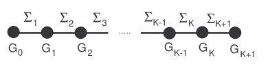
Figure 1: The diagram illustrates a deconstructed theory described by the gauge groups $G_{i}$ and by the chiral fields $\Sigma_{i}$.

2 2. Breaking the EW Symmetry without Higgs Fields

As we have seen in the previous Section, abstracting from the 5-dimensional example one can study more general moose geometries. The general structure will consist in many copies of the gauge group $G$ intertwined by link variables $\Sigma$. Now suppose that we want to describe the electro-weak (EW) symmetry breaking in this context. The condition we have to satisfy is that, before the EW gauge group is introduced, 3 massless Goldstone bosons should be present (to give masses to $W^{\pm}$ and $Z$) and all the moose gauge fields should be massive. In the simplest case we take all the moose gauge groups equal to $SU(2)$. Then, each $\Sigma$ field is an $SU(2)$ matrix

$$\Sigma_{i}=e^{i\vec{\pi}\cdot\vec{\tau}/(2f_{i})},$$ (12)

with $\vec{\tau}$ the Pauli matrices. Therefore each $\Sigma_{i}$ describes three spin zero fields ($\pi_{i}$). In a connected moose diagram any site (containing three gauge fields) may absorb one link (the 3 Goldstones $\pi_{i}$) giving rise to three massive gauge bosons. Therefore our condition translates into

$$number~{}of~{}links=number~{}of~{}sites+1.$$ (13)

The simplest of these moose is the ”linear moose” whose diagram is given in Fig. 2. The corresponding action is

$$S_{moose}=\int d^{4}x\left(-\sum_{i=1}^{K}\frac{1}{2}{\rm Tr}\left[F_{\mu\nu}^{i}F^{\mu\nu i}\right]+\sum_{i=1}^{K+1}f_{i}^{2}{\rm Tr}\left[\left(D_{\mu}\Sigma_{i}\right)\left(D^{\mu}\Sigma_{i}\right)^{\dagger}\right]\right).$$ (14)

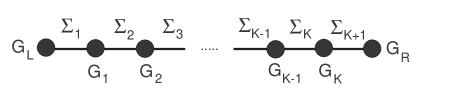
Figure 2: The simplest moose diagram for the Higgsless breaking of the EW symmetry.

We have now $K$ gauge groups $SU(2)$ and $K+1$ chiral fields. Notice that the model has two global symmetries $G_{L}$ and $G_{R}$ associated to the chiral fields $\Sigma_{1}$ and $\Sigma_{K+1}$

$$\Sigma_{1}\to U_{L}\Sigma_{1},~{}~{}~{}\Sigma_{K+1}\to\Sigma_{K+1}U_{R}^{\dagger}.$$ (15)

As such they have been associated to the ends of the moose in Fig. 2. It is this global symmetry, $G_{L}\otimes G_{R}=SU(2)_{L}\otimes SU(2)_{R}$, that is gauged by the standard group $SU(2)_{L}\otimes U(1)$, in order to give the standard massive gauge bosons $W^{\pm}$ and $Z$ and the massless photon. In fact, the three Goldstones remaining after that the moose gauge fields have eaten up the chiral fields are just the ones necessary for the breaking of the EW symmetry. Prototypes of this theory are the BESS model for $K=1$ Casalbuoni et al. (1985) and its generalizations Casalbuoni et al. (1989).

3 3. EW Corrections for the Linear Moose

If the moose vector fields are heavy enough it is possible to derive an effective action describing only the Standard Model (SM) fields. By denoting the typical mass of the moose vector fields by $M_{V}$, at the leading order in $(M_{W}/M_{V})^{2}$ one gets the usual SM relations

$$M_{W}^{2}=\frac{v^{2}}{4}g^{2},~{}~{}~{}M_{Z}^{2}=\frac{M_{W}^{2}}{c_{\theta}^{2}},~{}~{}~{}e=gs_{\theta}=g^{\prime}c_{\theta},$$ (16)

with ($v\approx 250~{}GeV$)

$$\frac{4}{v^{2}}\equiv\frac{1}{f^{\,2}}=\sum_{i=1}^{K+1}\frac{1}{f_{i}^{,2}}.$$ (17)

In this class of models all the corrections from new physics arise from mixing of the SM vector bosons with the moose vector fields and therefore are oblique corrections. As well known the oblique corrections are completely captured by the parameters $S$, $T$ and $U$ Peskin and Takeuchi (1990, 1992) or, equivalently by the parameters $\epsilon_{i}$, $i=1,2,3$ Altarelli and Barbieri (1991); Altarelli et al. (1998). For the linear moose, the existence of the global symmetry (custodial) $SU(2)_{V}$ ensures that

$$\epsilon_{1}=\epsilon_{2}=0,$$ (18)

or, equivalently $U=T=0$.

To compute the new physics contribution to the electroweak parameter $\epsilon_{3}$ Altarelli and Barbieri (1991) we will make use of the dispersive representation given in Refs. Peskin and Takeuchi (1990, 1992) for the related parameter $S$ ($\epsilon_{3}=g^{2}S/(16\pi)$)

$$\epsilon_{3}=-\frac{g^{2}}{4\pi}\int_{0}^{\infty}\frac{ds}{s^{2}}Im\left[\Pi_{VV}(s)-\Pi_{AA}(s)\right],$$ (19)

where $g$ is the $SU(2)_{L}$ gauge coupling and $\Pi_{VV}(AA)$ is the current-current correlator

$$\int d^{4}xe^{-iq\cdot x}\langle J^{\mu}_{V(A)}J^{\nu}_{V(A)}\rangle=ig^{\mu\nu}\Pi_{VV(AA)}(q^{2})+(q^{\mu}q^{\nu}~{}{\rm terms}).$$ (20)

$J_{V/A\mu}$ are the vector and axial currents associated to the global symmetry $SU(2)_{L}\otimes SU(2)_{R}$, getting the following contributions from the moose vector fields

$$J_{V\mu}^{a}\Big{|}_{\rm vector~{}mesons} = f_{1}^{2}g_{1}A_{\mu}^{1a}+f_{K+1}^{2}g_{K}A_{\mu}^{Ka},$$

$$J_{A\mu}^{a}\Big{|}_{\rm vector~{}mesons} = f_{1}^{2}g_{1}A_{\mu}^{1a}-f_{K+1}^{2}g_{K}A_{\mu}^{Ka}.$$ (21)

It should be noticed that the $\epsilon_{3}$ parameter is evaluated with reference to the SM, and therefore the corresponding contributions should be subtracted. For instance the contribution of the pion pole to $\Pi_{AA}$, that is of the Goldstone particles giving mass to the $W$ and $Z$ gauge bosons, does not appear in $\epsilon_{3}$. As described previously, in the model described by the action (14) all the new physics contribution comes from the new vector bosons (we are assuming the standard couplings for the fermions to $SU(2)_{L}\otimes U(1)$). Therefore from

$$Im\,\Pi_{VV(AA)}=-\pi\sum_{Vn,An}g^{2}_{nV,nA}\delta(s-m^{2}_{n}),$$ (22)

we get

$$\epsilon_{3}=\frac{g^{2}}{4}\sum_{n}\left(\frac{g_{nV}^{2}}{m^{4}_{n}}-\frac{g^{2}_{nA}}{m^{4}_{n}}\right),$$ (23)

where $g_{nV/A}$ are the decay coupling constants of the moose vector fields defined by

$$\langle 0|J_{V\mu}^{a}|\tilde{A}^{n}_{b}(p,\epsilon)\rangle=g_{nV}\delta^{ab}\epsilon_{\mu},~{}~{}~{}\langle 0|J_{A\mu}^{a}|\tilde{A}^{n}_{b}(p,\epsilon)\rangle=g_{nA}\delta^{ab}\epsilon_{\mu},$$ (24)

and $\tilde{A}^{n}_{b}(p,\epsilon)$ are the mass eigenstates of the moose vector bosons. As shown in Casalbuoni et al. (2004) we can express $\epsilon_{3}$ in two equivalent ways (see also Hirn and Stern (2004); Georgi (2005))

$$\epsilon_{3}=g^{2}g_{1}g_{K}f_{1}^{\,2}f_{K+1}^{\,2}(M_{2}^{-2})_{1K}=g^{2}\sum_{i=1}^{K}\frac{(1-y_{i})y_{i}}{g_{i}^{2}},$$ (25)

where $M_{2}$ is the matrix of the square masses of the moose vector bosons, and

$$y_{i}=\sum_{j=1}^{i}x_{j},~{}~{}~{}x_{i}=\frac{f^{2}}{f_{i}^{2}},~{}~{}~{}\frac{1}{f^{2}}=\sum_{i=1}^{K+1}\frac{1}{f_{i}^{2}}~{}\Rightarrow~{}\sum_{i=1}^{K+1}x_{i}=1.$$ (26)

Since $0\leq y_{i}\leq 1$ it follows $\epsilon_{3}\geq 0$ (see also Hirn and Stern (2004); Barbieri et al. (2004); Chivukula et al. (2004)). As an example, let us take all the link couplings $f_{i}$ equal to a common value $f_{c}$, and the same for the gauge couplings $g_{i}=g_{c}$. Then (see also Foadi et al. (2004))

$$\epsilon_{3}=\frac{1}{6}\frac{g^{2}}{g_{c}^{2}}\frac{K(K+2)}{(K+1)}.$$ (27)

If we want to be compatible with the experimental data we need to get $\epsilon_{3}\approx 10^{-3}$. For $K=1$ this would require $g_{c}\geq 15.8g$, implying a strong interacting gauge theory in the moose sector. Notice also that insisting on a weak gauge theory would imply $g_{c}$ of the order of $g$, let us say $g_{c}\approx 2\div 5g$. Then the natural value of $\epsilon_{3}$ would be of the order $10^{-1}-10^{-2}$, incompatible with the experimental data.

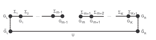
Figure 3: The diagram illustrates how a cut link model is generated from a linear moose.

Possible ways of evading the $\epsilon_{3}$ problem have been considered in Casalbuoni et al. (2004). A way is to cut a link, that is to assume one of the link couplings, say $f_{m}$, equal to zero. In this case the matrix of the mass square of the moose vector bosons becomes block diagonal and, as a consequence, the same happens for $M_{2}^{-2}$. Therefore $(M_{2}^{-2})_{1K}=0$ and $\epsilon_{3}=0$. Since, suppressing a link amounts to eliminate three scalar fields, we need a way to reintroduce them. The $\Sigma_{m}$ field can be reintroduced through a discretized version of a Wilson line

$$U=\Sigma_{1}\Sigma_{2}\cdots\Sigma_{K}\Sigma_{K+1},$$ (28)

and inserting in the lagrangian a term

$$f_{0}^{2}Tr[\partial_{\mu}U^{\dagger}\partial^{\mu}U].$$ (29)

This term has a global invariance $\tilde{G}_{L}\otimes\tilde{G}_{R}=SU(2)_{L}\otimes SU(2)_{R}$ originating from a transformation $U\to\tilde{U}_{L}U\tilde{U}_{R}$. This invariance is different from the original $G_{L}\otimes G_{R}$ before the EW gauging. As a consequence the model has an enhanced custodial symmetry $\left[SU(2)_{L}\otimes SU(2)_{R}\right]$ which is enough to ensure $\epsilon_{3}=0$ Inami et al. (1992). A particular example of this model, for $K=2$ ($D-BESS$), was studied in Casalbuoni et al. (1995, 1996) (originally introduced in Casalbuoni et al. (1989)).

Another possibility Casalbuoni et al. (2004) is to suppress a link, that is to assume a hierarchy among the links. As an example assume an exponential behavior

$$f_{i}=\bar{f}e^{c(i-1)},~{}~{}~{}~{}g_{i}=g_{c}.$$ (30)

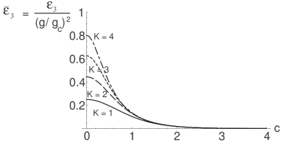
Figure 4: The behavior of $\epsilon_{3}$ (normalized to $(g/g_{c})^{2}$) as a function of $c$ in the exponentially suppressed linear model for different values of $K$.

From Fig. 4 we see that there is a big suppression factor, of order $10^{-2}$ already for $c=2$. In fact expanding at the leading order for large $c$ it is easily seen that

$$\epsilon_{3}\rightarrow\frac{g^{2}}{g_{c}^{2}}e^{-2c}.$$ (31)

However, lowering or cutting the links may give rise to unitarity problems. For instance, in the cut model $f_{0}$ must be of the order of the v.e.v. of the Higgs field in the SM making the unitarity limit of these class of model the same as in the SM without Higgs. We will study the unitarity limits of the moose models in the next Section.

4 4. Unitarity bounds for the linear moose

The worst high-energy behavior of the moose models arises from the scattering of longitudinal vector bosons. To simplify the calculation we will make use of the equivalence theorem, that is of the possibility of evaluating this amplitude in terms of the scattering amplitude of the corresponding Goldstone bosons Cornwall et al. (1974). However this theorem holds in the approximation where the energy of the process is much higher of the mass of the vector bosons. We will consider two situations. In the first one we assume that all the moose vectors have a mass, $M_{V_{i}}$, much higher than the SM vector boson masses, in such a way that we can evaluate the amplitude for the SM $W$ and $Z$ at energies $M_{W/Z}\ll E\ll M_{V_{i}}$. The only Goldstone bosons of interest here are the ones giving mass to $W$ and $Z$. The unitary gauge for these bosons is given by the choice

$$\Sigma_{i}=e^{if\vec{\pi}\cdot\vec{\tau}/(2f_{i}^{2})},$$ (32)

with $f$ given in eq. (17). The resulting four-pion amplitude is

$$A_{\pi^{+}\pi^{-}\to\pi^{+}\pi^{-}}=-\frac{f^{4}u}{4}\sum_{i=1}^{K+1}\frac{1}{f_{i}^{6}}+\frac{f^{4}}{4}\sum_{i,j=1}^{K}L_{ij}\left((u-t)(s-M_{2})_{ij}^{-1}+(u-s)(t-M_{2})_{ij}^{-1}\right),$$ (33)

with

$$L_{ij}=g_{i}g_{j}\left(\frac{1}{f_{i}^{2}}+\frac{1}{f_{i+1}^{2}}\right)\left(\frac{1}{f_{j}^{2}}+\frac{1}{f_{j+1}^{2}}\right).$$ (34)

This expression reproduces correctly the low-energy limit, $E\ll M_{V_{i}}$:

$$A_{\pi^{+}\pi^{-}\to\pi^{+}\pi^{-}}\to-\frac{f^{4}u}{4}\left(\sum_{i=1}^{K+1}\frac{1}{f_{i}^{2}}\right)^{3}=-\frac{u}{4f^{2}}=-\frac{u}{v^{2}},$$ (35)

whereas in the high-energy limit, where we can neglect the second term,

$$A_{\pi^{+}\pi^{-}\to\pi^{+}\pi^{-}}=-\frac{f^{4}u}{4}\sum_{i=1}^{K+1}\frac{1}{f_{i}^{6}}.$$ (36)

The best unitarity limit is obtained for all the $f_{i}$’s being equal to a common value $f_{c}$. In this case

$$A_{\pi^{+}\pi^{-}\to\pi^{+}\pi^{-}}=-\frac{u}{(K+1)v^{2}},$$ (37)

leading to the unitarity bound

$$\Lambda_{moose}=(K+1)\Lambda_{HSM}\approx 1.2(K+1)~{}TeV,$$ (38)

where $\Lambda_{HSM}$ is the unitary bound for the Higgsless SM. In this case it is possible to improve as much as we like the unitarity bound of the SM increasing $K$. However this would lead to contradictions with the experimental bounds on $\epsilon_{3}$.

As a second instance we consider an energy much higher than all the masses of the vector bosons. In this case to determine the unitarity bounds one has to consider the eigenchannel amplitudes corresponding to all the possible four-longitudinal vector bosons. But, since the unitary gauge for all the vector bosons is simply given by the expression (12), the amplitudes are already diagonal, and the result at high energy is simply

$$A_{\pi^{+}\pi^{-}\to\pi^{+}\pi^{-}}\to-\frac{u}{4f_{i}^{2}}.$$ (39)

We see that the unitarity limit is determined the smallest link coupling. Therefore in the exponentially suppressed model the unitarity bound is essentially the same as in the SM, since in order to respect the constraint given by the first equality in eq. (17), the lowest coupling must be of order $v$. Also in this case the best unitarity limit is for all the link couplings being equal $f_{i}=f_{c}$. Then (for similar results see Chivukula and He (2002))

$$\Lambda_{moose}=\sqrt{K+1}\Lambda_{HSM}\approx 1.2\sqrt{K+1}~{}TeV.$$ (40)

However, in order our approximation is correct we have to require $M_{V_{i}}^{max}\ll\Lambda_{moose}$, and since we expect roughly (assuming $g_{c}\approx g$) $M_{V_{i}}^{max}\approx KM_{W}$, we get a bound $\sqrt{K}\ll 14$. By taking $\sqrt{K}$ of order $2\div 3$ one could improve of the same factor the SM unitarity bound, but again this would be hardly compatible with the electro-weak experimental data.

5 5. Delocalizing fermions

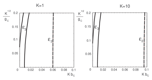
Figure 5: The 95% C.L. allowed region in the plane $(Kb_{c},\sqrt{K}/g_{c})$ is the region on the left delimited by the two continuous lines coming form the bounds on $\epsilon_{3}$. The dashed line comes from a bound on $\epsilon_{2}$, whereas the other bound form $\epsilon_{2}$ and the bounds from $\epsilon_{1}$ are out of the figure. The radiative corrections have been assumed as in the SM with $m_{H}=1~{}TeV$ and $m_{top}=178~{}GeV$.

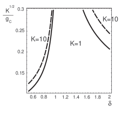
Figure 6: The 95% C.L. allowed regions in the plane $(\delta,\sqrt{K}/g_{c})$ are the ones at the interior of the lines corresponding to $K=1$ (continuous) and $K=10$ (dashed). The radiative corrections have been chosen as in Fig. 5.

As we have seen, it is not possible to satisfy at the same time the experimental bounds on $\epsilon_{3}$ and improve in a sensible way the unitarity limit. A way out has been considered in Casalbuoni et al. (2005); Chivukula et al. (2005a, b) allowing delocalized couplings of the SM fermions to the moose gauge fields and some amount of fine tuning. In fact, the SM fermions can be coupled to any of the gauge fields staying at the lattice sites by means of a Wilson line. However, we will consider only left-handed fermions, since analogous interactions for the right-handed ones are very much constrained Casalbuoni et al. (1985, 1987). Define

$$\chi_{L}^{i}=\Sigma_{i}^{\dagger}\Sigma_{i-1}^{\dagger}\cdots\Sigma_{1}^{\dagger}\psi_{L}.$$ (41)

Then, under a gauge transformation, $\chi_{L}^{i}\to U_{i}\chi_{L}^{i}$, with $U_{i}\in G_{i}$. We see that at each site we can introduce a gauge invariant coupling given by

$$b_{i}\bar{\chi}_{L}^{i}\gamma^{\mu}\left(\partial_{\mu}+ig_{i}A_{\mu}^{i}+\frac{i}{2}g^{\prime}(B-L)Y_{\mu}\right)\chi_{L}^{i}.$$ (42)

The expressions for the parameters $\epsilon_{i}$ are modified, and at first order in the couplings $b_{i}$ we get

$$\epsilon_{1}\approx 0,~{}~{}~{}\epsilon_{2}\approx 0,~{}~{}~{}\epsilon_{3}\approx\sum_{i=1}^{K}y_{i}\left(\frac{g^{2}}{g_{i}^{2}}(1-y_{i})-b_{i}\right).$$ (43)

Therefore, with some amount of fine tuning is possible to agree with the electro-weak experimental data. To show it, let us take again all the link couplings equal to $f_{c}$ and the gauge couplings equal to $g_{c}$. We have considered two possibilities. In the first one we take also the $b_{i}$ equal to a common value $b_{c}$. Then the allowed region in the space $(Kb_{c},\sqrt{K}/g_{c})$ (we have chosen these parameters due to the scaling properties of $g_{c}$ and $b$ with $K$) is given in Fig. 5.

In the second case we require a sort of local cancelation, assuming (again $g_{i}=g_{c}$, $f_{i}=f_{c}$)

$$b_{i}=\delta\frac{g^{2}}{g_{i}^{2}}(1-y_{i})=\delta\frac{g^{2}}{g_{c}^{2}}\left(1-\frac{i}{K+1}\right).$$ (44)

The allowed region in the space $(\delta,\sqrt{K}/g_{c})$ is given in Fig. 6. In this way it is possible to satisfy the EW constraints and improve the unitarity bound of the Higgsless SM at the same time.

References

- Arkani-Hamed et al. (1998) N. Arkani-Hamed, S. Dimopoulos, and G. R. Dvali, Phys. Lett. B429, 263 (1998), hep-ph/9803315.
- Antoniadis et al. (1998) I. Antoniadis, N. Arkani-Hamed, S. Dimopoulos, and G. R. Dvali, Phys. Lett. B436, 257 (1998), hep-ph/9804398.
- Hill et al. (2001) C. T. Hill, S. Pokorski, and J. Wang, Phys. Rev. D64, 105005 (2001), hep-th/0104035.
- Cheng et al. (2001) H.-C. Cheng, C. T. Hill, S. Pokorski, and J. Wang, Phys. Rev. D64, 065007 (2001), hep-th/0104179.
- Arkani-Hamed et al. (2001a) N. Arkani-Hamed, A. G. Cohen, and H. Georgi, Phys. Rev. Lett. 86, 4757 (2001a), hep-th/0104005.
- Arkani-Hamed et al. (2001b) N. Arkani-Hamed, A. G. Cohen, and H. Georgi, Phys. Lett. B513, 232 (2001b), hep-ph/0105239.
- Casalbuoni et al. (1985) R. Casalbuoni, S. De Curtis, D. Dominici, and R. Gatto, Phys. Lett. B155, 95 (1985).
- Casalbuoni et al. (1989) R. Casalbuoni, S. De Curtis, D. Dominici, F. Feruglio, and R. Gatto, Int. J. Mod. Phys. A4, 1065 (1989).
- Peskin and Takeuchi (1990) M. E. Peskin and T. Takeuchi, Phys. Rev. Lett. 65, 964 (1990).
- Peskin and Takeuchi (1992) M. E. Peskin and T. Takeuchi, Phys. Rev. D46, 381 (1992).
- Altarelli and Barbieri (1991) G. Altarelli and R. Barbieri, Phys. Lett. B253, 161 (1991).
- Altarelli et al. (1998) G. Altarelli, R. Barbieri, and F. Caravaglios, Int. J. Mod. Phys. A13, 1031 (1998), hep-ph/9712368.
- Casalbuoni et al. (2004) R. Casalbuoni, S. De Curtis, and D. Dominici, Phys. Rev. D70, 055010 (2004), hep-ph/0405188.
- Hirn and Stern (2004) J. Hirn and J. Stern, Eur. Phys. J. C34, 447 (2004), hep-ph/0401032.
- Georgi (2005) H. Georgi, Phys. Rev. D71, 015016 (2005), hep-ph/0408067.
- Barbieri et al. (2004) R. Barbieri, A. Pomarol, and R. Rattazzi, Phys. Lett. B591, 141 (2004), hep-ph/0310285.
- Chivukula et al. (2004) R. S. Chivukula, M. Kurachi, and M. Tanabashi, JHEP 06, 004 (2004), hep-ph/0403112.
- Foadi et al. (2004) R. Foadi, S. Gopalakrishna, and C. Schmidt, JHEP 03, 042 (2004), hep-ph/0312324.
- Inami et al. (1992) T. Inami, C. S. Lim, and A. Yamada, Mod. Phys. Lett. A7, 2789 (1992).
- Casalbuoni et al. (1995) R. Casalbuoni et al., Phys. Lett. B349, 533 (1995), hep-ph/9502247.
- Casalbuoni et al. (1996) R. Casalbuoni et al., Phys. Rev. D53, 5201 (1996), hep-ph/9510431.
- Cornwall et al. (1974) J. M. Cornwall, D. M. Levin, and G. Tiktopoulos, Phys. Rev. D11, 1145 (1974).
- Chivukula and He (2002) R. S. Chivukula and H.-J. He, Phys. Lett. B532, 121 (2002), hep-ph/0201164.
- Casalbuoni et al. (2005) R. Casalbuoni, S. De Curtis, D. Dolce, and D. Dominici, Phys. Rev. D71, 075015 (2005), hep-ph/0502209.
- Chivukula et al. (2005a) R. S. Chivukula, E. H. Simmons, H.-J. He, M. Kurachi, and M. Tanabashi, Phys. Rev. D71, 115001 (2005a), hep-ph/0502162.
- Chivukula et al. (2005b) R. S. Chivukula, E. H. Simmons, H.-J. He, M. Kurachi, and M. Tanabashi, Phys. Rev. D72, 015008 (2005b), hep-ph/0504114.
- Casalbuoni et al. (1987) R. Casalbuoni, S. De Curtis, D. Dominici, and R. Gatto, Nucl. Phys. B282, 235 (1987).